Building Energy Management Using Increased Thermal Capacitance and Thermal Storage Management


Department Mechanical Engineering, Mississippi State University, Starkville, MS 39762, USA
*
Author to whom correspondence should be addressed.
Buildings 2018, 8(7), 86; https://doi.org/10.3390/buildings8070086
Submission received: 1 June 2018
/
Revised: 21 June 2018
/
Accepted: 25 June 2018
/
Published: 27 June 2018
Abstract
:This study simulates an increased thermal capacitance (ITC) and thermal storage management (TSM) system to reduce the energy consumed by air conditioning and heating systems. The ITC/TSM is coupled with phase change materials (PCM), which enable tank volume reduction. The transient energy modeling software, the Transient System Simulation Tool (TRNSYS), is used to simulate the buildings’ thermal response and energy consumption, as well as the ITC/TSM system and controls. Four temperature-controlled operating regimes are used for the tank: building shell circulation, heat exchanger circulation, solar panel circulation, and storage. This study also explores possible energy-saving benefits from tank volume reduction such as losses associated with the environment temperature due to tank location. Three different tank locations are considered in this paper: outdoor, buried, and indoor. The smallest tank size (five gallons) is used for indoor placement, while the large tank (50 gallons) is used either for outdoor placement or buried at a depth of 1 m. Results for Atlanta, Georgia show an average 48% required energy decrease for cold months (October–April) and a 3% decrease for warm months (May–September) for the ITC/TSM system with PCM when compared with the reference case. A system with PCM reduces the tank size by 90% while maintaining similar energy savings.
1. Introduction
For the residential sector in the South Atlantic portion of the United States (US), building energy consumption related to air conditioning and heating make up 42% of a building’s total energy usage, where air conditioning constitutes 13% and space heating constitutes 29% [1]. Reducing energy consumption not only has a positive effect on the resident through decreased operating costs, it also has a possible environmental impact by decreasing dependence on natural resources such as coal and natural gas.
Due to this possible benefit, the US state of Georgia was chosen for simulations due to a high dependency on nonrenewable resources for electricity generation. Only 6.6% of the electricity produced by Georgia is from renewable energy sources, while the national average is around 16% [2]. This location could provide a larger opportunity for reducing carbon emissions than those states with a higher usage of renewable energy sources.
Methods for providing thermal comfort with no or little additional cost are often referred to as passive methods. Passive energy saving methods comprise a large variety of implementations; examples of such are building orientation and shading [3], and indirect and direct heat storage. In indirect heat storage, gains can come from concepts such as a Tromba wall, water wall, or solarium, while in direct heat storage, heat enters the building through windows and walls [4]. These methods are limited to natural modes of heat transfer such as free convection and conduction. Shaviv et al. [5] studied the passive influence of thermal mass in hot humid locations by performing simulations using four variations of building materials. They found that buildings with a large thermal mass were able to reduce the internal building temperature by 3–6 °C without air conditioning (AC) operation.
Other research using building thermal mass for energy reduction have been well documented [6,7,8,9,10,11,12,13]. The thermal inertial of a building is one of the controlling factors for the phase shift and amplitude reduction of “heat flow fluctuations” associated with the building’s internal temperature response due to weather [11]. Aste et al. [12] found that buildings with external walls of a high thermal capacitance could results in lower heating and cooling demand, with peak savings of around 10% for heating and 20% for cooling. However, Reilly et al. [8] found that for cold climates, a large thermal mass could be a hindrance, and should be coupled with preheating strategies. Simulations by Slee et al. [13] showed an exponential relationship between thermal capacitance and the fluctuation of the daily internal building temperature. This illustrates that there is point at which increasing the thermal mass for a specific system would not provide any addition in benefits. The study presented in this paper uses an active mode of increased thermal capacitance along with temperature-driven controllers to manage the thermal capacitance.
The works previously mentioned above use only passive methods for additional thermal mass. If these methods used permanent installations, such as buildings constructed with a high thermal mass, then benefits could have been lost when a low thermal capacitance is favorable. Due to this, investigations into active thermal mass and thermal storage methods are of interest [14,15,16,17,18,19]. Carpenter et al. [16] found building energy consumption reduced when implementing increased thermal capacitance though water circulation in the shell of the building. They found the greatest energy reduction (11%) when circulation included the ceiling, which is in the model for this paper. A review performed by Navarro et al. [14] found benefits associated with active methods for thermal energy storage (TES), but also stated that thermal water tanks have limited potential due to the impractical amount of space required. This paper aims to address this issue by introducing phase change materials (PCM) to a water storage tank to reduce tank size with only small reductions to heat storage capacity. Kong et al. [18] and Whiffen et al. [15] both conducted experiments showing the validity of integrating PCMs for increased thermal mass, Kong et al. through passive PCM wallboards, and Whiffen et al. though an active hollow slab with embedded PCM. Whiffen et al. were able to show a delay in AC onset by 1.2 h. The impact of PCM on building energy consumption has also been studied using numerical simulations using software such as the Transient System Simulation Tool (TRNSYS [20]) [21,22,23,24], which was also used in this paper’s study.
The purpose of this study was to investigate active increased thermal capacitance and thermal storage using a water loop system. Temperature control systems were also included to increase benefits when possible, and PCM was used to reduce the size of the water tank.
2. Reference Model
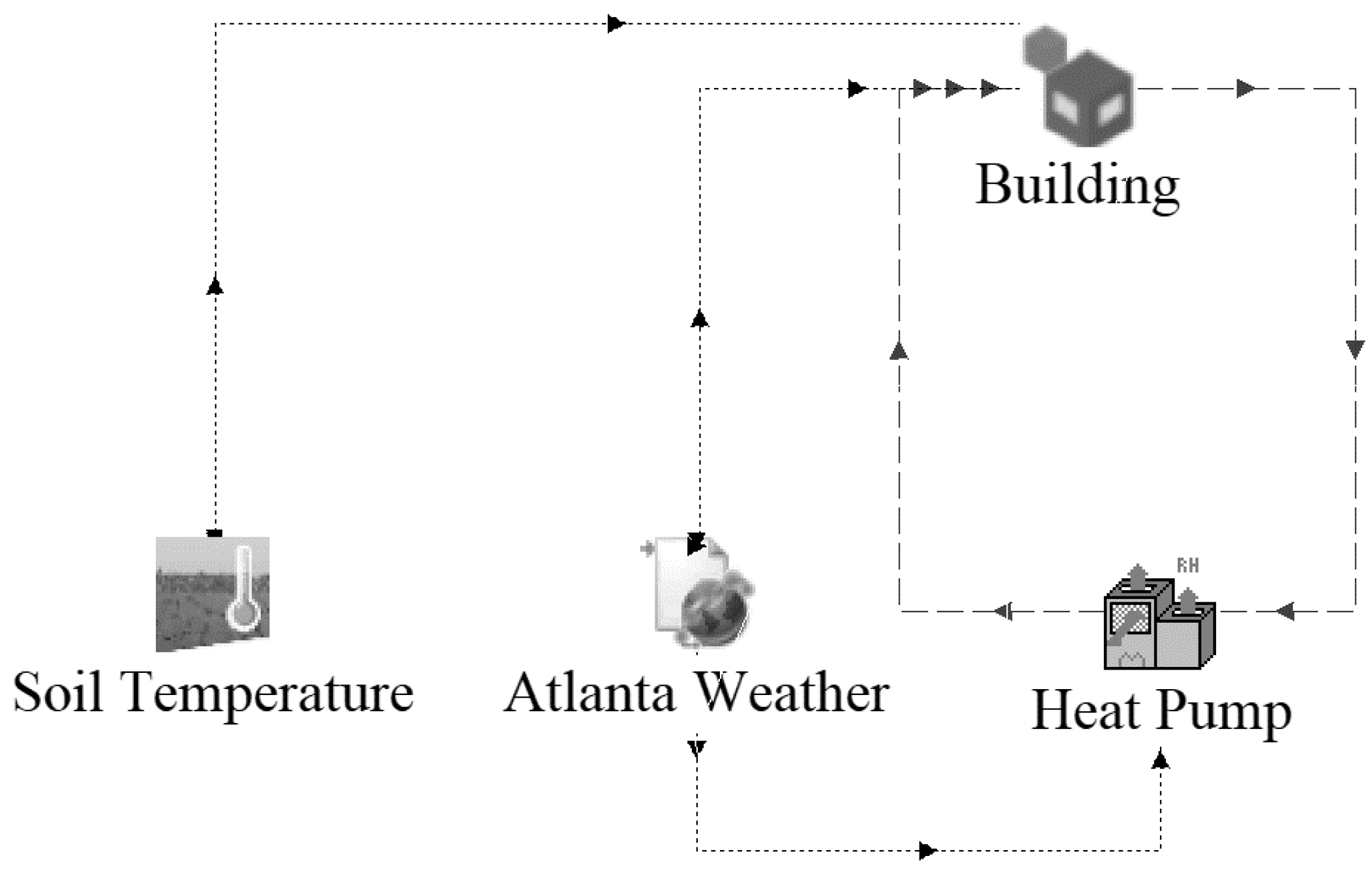
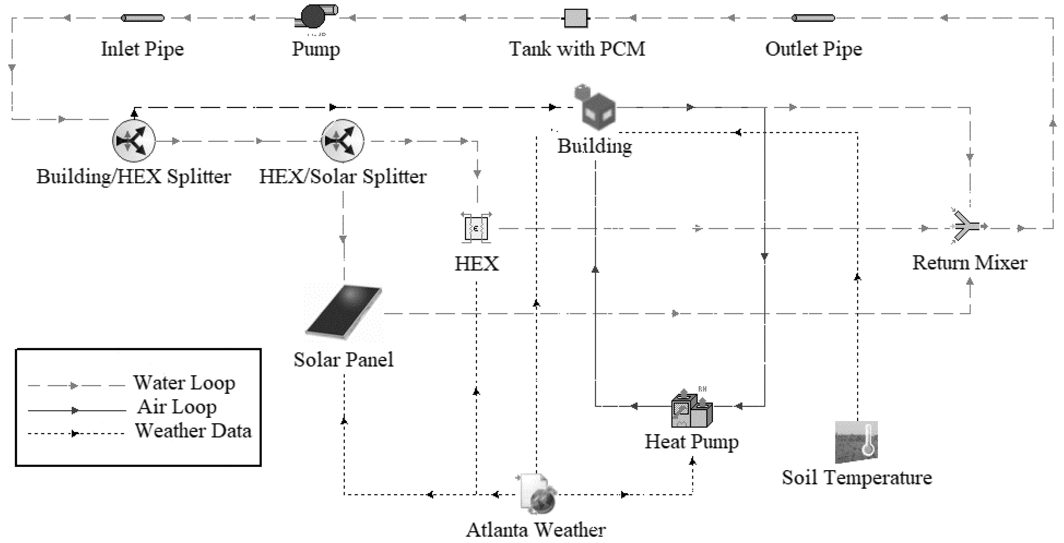
A reference model was simulated to provide a basis to compare the ITC/TSM system. All of the building materials, simulation parameters, and weather data listed in Section 2.1 and Section 2.2 were kept constant for all of the simulations. This was done to isolate the effect of the water tank on the building air conditioning load requirement. The heating and cooling system was also unchanged between simulations. Figure 1 shows the TRNSYS schematic used for the reference model simulations.
2.1. Building Specifications and Location
A small single room wood-sided building with a concrete slab was selected for the simulations. It was intended to have a similar size as a small/medium apartment or small office building. The building had a floor plan of 100 m2 (1300 ft2) and 3-m (10 ft) high ceiling. Surfaces were chosen from the TRNSYS library, which contains typical wall constructions [25]. Materials were chosen to simulate lightweight buildings that are common in the southeastern part of the US. The wall, ceiling, and floor building materials and thickness are listed in Table 1.
Additionally, the building was ground coupled to allow heat transfer through the floor of the building. This was done by calculating the soil temperature at the depth of the slab foundation and allowing this to be the thermal boundary condition for the bottom side of the slab. An approximation for the soil temperature was obtained using Kusuda’s equation [26].
where Tmean is the average annual air temperature, Tamp is the maximum air temperature minus the average air temperature, d is the depth of the desired temperature, α is the soil thermal diffusivity, t is the day at which the temperature is found, and tshift is the day of year associated with the minimum air temperature. The values used for Atlanta, Georgia are given in Table 2.
Weather information was selected from Typical Meteorological Year 2 (TMY2) data for Atlanta, Georgia. The following is the weather information used from TMY2 data: dry bulb temperature, percent relative humidity, and atmospheric pressure. TRNSYS Type 15 was used in conjunction with TMY2 data to calculate total radiation, beam radiation, and angle of incidence of beam solar radiation each surface as well as the effective sky temperature, humidity ratio, and ground reflectance. The walls of the building were identical and were oriented at azimuth angles of 0°, 90°, 180°, and 270°. Each external wall of the building had a 0.5 m2 insulated window. These windows had a u-value of 1.3 and a g-value of 0.591.
Natural convection was assumed as the boundary condition of the internal walls, and an averaged forced convection was assumed for external walls. A standard value was used for the convective heat transfer coefficient, which was 3 W/m2 K for the internal wall side, and 24 W/m2 K for the external wall side [25]. For increased thermal capacitance (ITC)/thermal storage management (TSM) cases, automatic calculation was allowed to determine the inside heat transfer coefficient. This was because the internal heating or cooling of the wall can impact the surface temperature on which the natural convection heat transfer coefficient is dependent.
2.2. Heat Pump Parameters
A small air source heat pump was chosen to provide the heating and cooling requirements for the building. It was modeled using TRNSYS TESS (Thermal Energy System Specialists) Library component 954 with the percent relative humidity mode for moist air calculations. This component uses normalized capacity, sensible capacity, and power tables to calculate both the heating and cooling rates. The parameters for the selected heat pump were chosen from a commercially available split system heat pump data sheet, and are shown in Table 3.
From ASHRAE Standards 62.1 and 62.2 [27], the required fresh air CFM (cubic foot per minute) per person for an office building is 17, and for an apartment building is 7.5. Therefore, 17 CFM/person was used in all of the simulations. Using this value, an air flow rate of 1200 CFM, and an outside damper position of 30% allows for up to 21 people to occupy the building at a single time.
Two different climate seasons were considered: a heating season and a cooling season. The heating season was set from 1 November to 31 March, and the cooling season was set from 1 April to 31 October. The thermostat setting included a setting for daytime and evening operation, and a 2 °C deadband around the nominal setting. Evening was considered to last from 8 p.m. to 8 a.m., and daytime was considered to last from 8 a.m. to 8 p.m. For the cooling season, a step-up temperature was applied during the daytime, and for the heating season, a step-back temperature was applied during the daytime. This was done to simulate how an individual might control the AC/heat when the building was not occupied to reduce operating costs. Values for the thermostat are listed in Table 4.
During the heating season, the air condition operated if the indoor temperature was above 24 °C (75.5 °F), and during the cooling season, the heater operated if the indoor temperature was below 18.5 °C (65.5 °F). Due to the nature of the southeast US weather, the conditions that allowed the heat pump to operate during the cooling season and the AC to operate during the heating season only occurred during the mild months of the year, which were April, May, and September.
3. ITC/TSM Model with PCM
The increased thermal capacitance and thermal storage management (ITC/TSM) model expanded upon the reference case by addition of a water loop system. Copper pipes embedded in the walls and ceiling of the building used water circulation to increase the thermal capacitance of the building, and thus increased the overall time constant of the building. Variations in the building’s thermal time constant for each model are discussed in Section 3.3.
This water loop for this system comprised a hydraulic pump, water tank, heat exchanger (HEX), solar panel, valves, and copper pipes embedded in the walls and ceiling of the building. Figure 2 shows the TRNSYS schematic for the ITC/TSM model.
An air-to-water constant effectiveness cross-flow heat exchanger was chosen to be the main method of cooling the water during the warm season. This HEX, along with a low value for effectiveness (0.4), was chosen to give conservative results. The temperature of the air stream corresponded to the outdoor conditions.
The water did not circulate through all four devices in a single cycle, but was diverted by two temperature and season-controlled valves. The HEX and solar panel were used to regulate the water temperature when climate conditions were beneficial. A seasonal switch was also implemented to only allow HEX circulation during the cooling season and solar panel circulation during the heating season. The purpose of this method was to add a non-temperature restriction on circulation. This approach kept the water from attempting to cool during the winter and heat during the summer. The switch operated on a monthly basis, which was associated with the heating/cooling seasons. Building circulation was always a priority; when the building could not benefit from water circulation and the outdoor climate was not favorable, the pump shut off and the water was stored in the tank (which was subject to losses to the surroundings). The requirements for these valves are listed in Table 5.
A large water tank was used to significantly increase the time constant of the building [19]. To retain a large thermal time constant and reduce the size of the tank, a phase change material (PCM) was added. Only water was circulated through the loop; the PCM remained in the tank. For simulation purposes, it was assumed that the phase change material was perfectly mixed in the water tank. The HEX and solar panel were used to heat or cool the water that cycles back to the PCM. This process kept the water temperature oscillating within the small temperature band close to the melting point of the PCM.
To implement the PCM in TRNSYS, a vertical cylinder fluid storage tank with a single inlet and outlet was modified. Seven user input parameters were added: percent of tank volume that is PCM, PCM solid and liquid density, PCM solid and liquid specific heat, melting temperature, and heat of fusion.
The program for the vertical thermal storage was modified in various ways. A crucial addition was the numerical approximation for the PCM’s properties. This was done using a method demonstrated by Voller [28], which proposed that the phase change happens over a small temperature range instead of isothermally. This allowed the specific heat of a phase change material to be approximated by a piecewise function as seen in Equation (1):
where is the specific heat for the solid PCM with units of J/kg K, is the specific heat of the liquid PCM with units of J/kg K, LHF is the latent heat of fusion with units of J/kg, and ϵ is the small temperature interval over which phase change occurs with units of K. Selection of the temperature interval ϵ is discussed by Voller [28]. A graphical representation of the specific heat’s relationship to temperature and enthalpy is shown in Figure 3.
Other modifications included the reduction of water mass when PCM was added to the tank. Equation (2) is the water mass on a nodal basis:
where is the cross-sectional area of the tank for each node with units of m2, is the tank height of each node with units of m, is the density of water with units of kg/m3, and is the percentage of the tank volume occupied by the PCM.
Equation (3) represents the mass of PCM on a nodal basis:
To determine the mass of PCM, the density of the solid state was used. It was assumed that the PCM was solid when calculating the volume occupied in the tank.
Equation (4) is the modified nodal stored internal energy to include the PCM:
where is the temperature at each node with units of K, is the specific heat of water with units of J/kg K, and is the temperature-dependent specific heat of the PCM. This value is only reported when calculating the internal energy change i.e., where is the internal energy at the beginning of the simulation.
The heat equation (Equation (5)) for the ith tank segment was also altered to include the phase change mass and specific heat. The specific heat for the PCM is evaluated at the previous timestep.
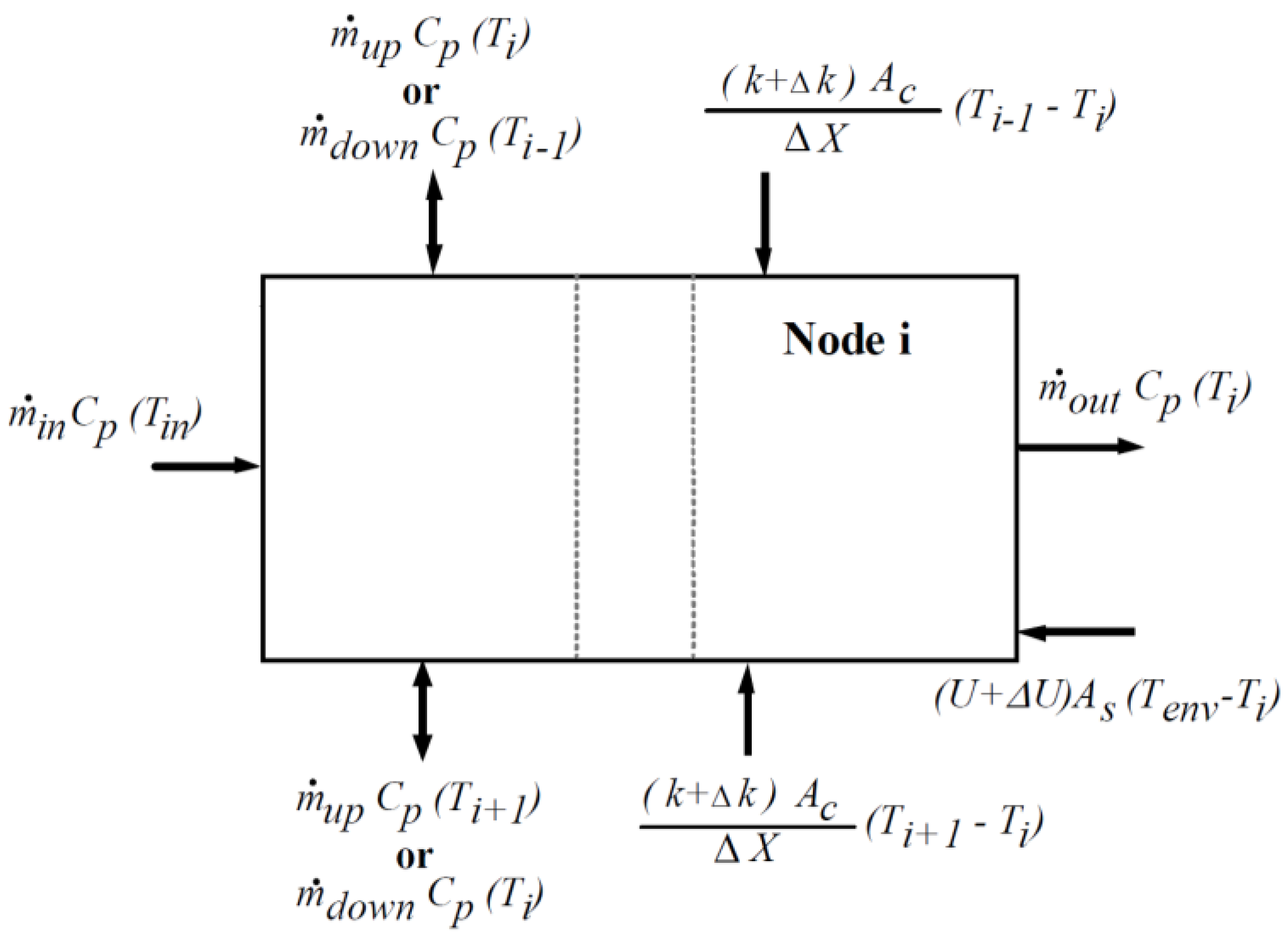
where, is the center-to-center distance between node i and the node below it (i + 1) in m, is the center-to-center distance between node i and the node above it (i − 1) in m, is the thermal conductivity of water with units of W/mK, is the loss coefficient (per unit area) of the tank with units of W/m2 K, is the surface area of node i in m2, is the environment temperature in K, and are the bulk fluid flowrate down/up the tank in kg/s, and and are the mass flowrate entering at the inlet and leaving at the outlet in kg/s.
This can be seen in a graphical representation of the energy flow into each node in Figure 4, which was taken from the mathematical reference [29] provided by TRNSYS for Type 60.
Only the internal energy of the tank’s ith segment was altered to include the PCM, since the PCM is not part of the flow energy transfer. The conduction of the phase change materials in each segment is included in the numerical approximation of the specific heat.
A generic paraffin PCM was chosen for simulations because of the stability in thermal cycling and the high heat of fusion [30]. Typical values of heat of fusions range from 200 kJ/kg to 280 kJ/kg; the specific heat is around 2 kJ/kg K, solid density is around 900 kg/m3, and melting temperatures range from −20 °C to 100 °C [30]. Preliminary simulations found benefits peaked for a melting temperature of 21.5 °C.
Values were chosen for the PCM using the generic paraffin ranges, and are presented in Table 6.
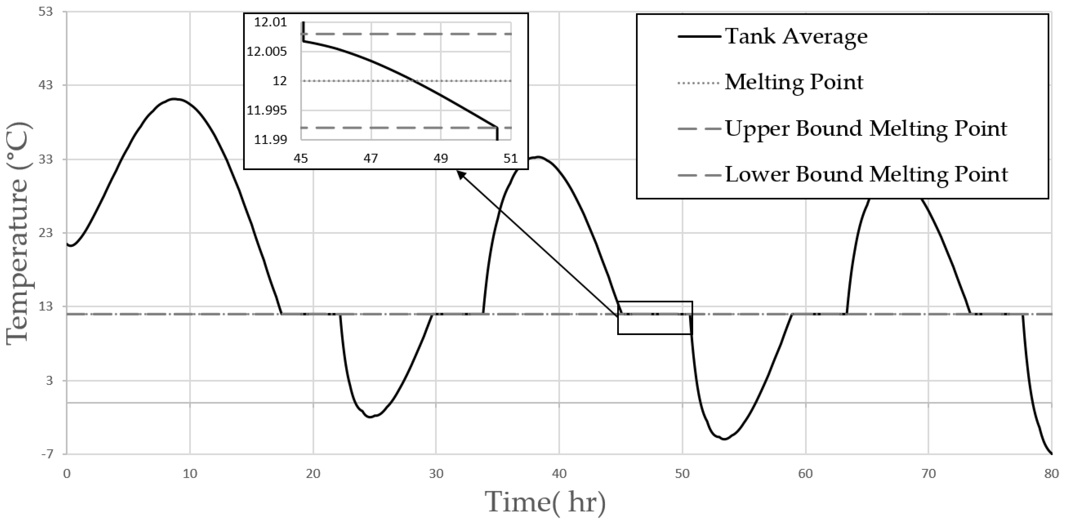
3.1. Verification of PCM Tank Operation
To verify that the specific heat modifications were working correctly, the tank was isolated with only a sinusoidal temperature input and constant flowrate. Figure 5 shows the average tank temperature, the PCM melting temperature, and the upper and lower bounds for phase chase. It can easily be seen how the temperature slowly decreased over 0.016 °C (ϵ = 0.008 °C) during phase change. This simplified mode is only shown for verification that the tank specific heat piecewise equation (i.e., Equation (1)) was operating as intended.
3.2. TRNSYS Solar Panel Selection
A 2 m2 flat plate solar panel was selected and the parameters were found from a Solar Rating and Certification Corporation (SRCC) data sheet [31]. The TRNSYS TESS component 539 was used to model the solar panel in simulations. This was chosen for the ability to internally modulate the flowrate for outlet temperature control. If the collector was gaining energy, the flowrate varied between a user-defined maximum and minimum flowrate to attempt to deliver a desired outlet temperature. If this temperature could not be maintained, the collector would run at the minimum flowrate, and would automatically shut off if the collector was losing energy.
Minor modifications were made to the TRNSYS TESS component; the maximum flowrate was redefined as an input variable instead of a parameter. This allowed the maximum flowrate to change at each timestep. The maximum flowrate was set to the inlet flowrate to the solar panel; this method kept the solar panel from operating when the input flowrate was zero, and allowed it to stay on as long as the collector was gaining energy. The parameters for the solar panel are listed in Table 7.
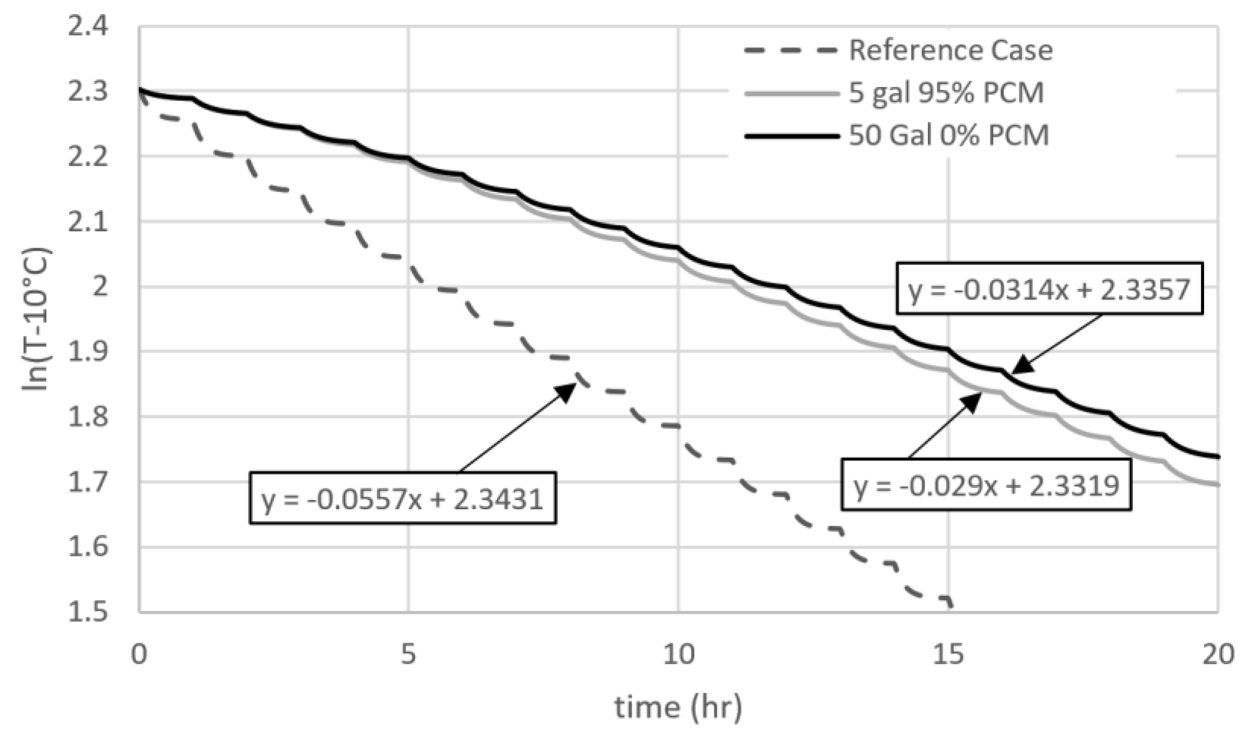
3.3. Verification of Building Thermal Time Constant Increment
To confirm that the dominant time constant of the building increased when implementing the ITC/TSM system, a free response simulation was conducted. Equation (6) was used to model the response of each case.
where is the time constant, C is the constant weather temperature, and A is a constant of integration.
The above equation was rearranged to solve for the time constant τ.
The inverse of the slope of Equation (7) yields the dominant time constant for the building. For each case, the building’s free response was found, and was plotted versus time. These slopes and their respective linear trendline equations can be seen in Figure 6.
The time constant of the reference case was 18 h, for the 50-gallon tank ITC/TSM case was 34.4 h, and for the five-gallon ITC/TSM with 95% phase change materials was 31.8 h. Thus, the PCM allowed for a 90% reduction in tank volume size with a very small reduction in the dominant time constant of the building.
3.4. Energy Balance
An energy balance was conducted for each major component in the simulation to ensure that the modifications to the water tank and the solar panel did not result in any unbalanced energy equations. A certain amount of error is expected for numerical simulations; therefore, the percentage of unbalanced energy is reported in the results section.
3.4.1. Water Tank
When examining the water tank, all of the thermal losses to the ambient conditions were neglected. Equation (8) was used to calculate the unbalanced energy rate for the water tank.
where is the unbalanced energy rate of the water tank, and are the energy removed by the outlet and energy supplied by the inlet as calculated internally by TRNSYS with units of kJ/h, is the specific heat of water with units of kJ/kgK, and are the mass flowrate associated with the outlet and inlet with units of kg/h, and and are the inlet and outlet temperatures in K.
For the water tank, 0.2% of timesteps did not satisfy the energy balance; however, after numerical integration of the energy rate, the energy associated with these timesteps only accounted for 0.00012% of the total energy transferred into or out of the tank subsystem.
3.4.2. Solar Panel
The solar panel energy balance was checked using Equation (9).
where is the TRNSYS internal calculation of energy gained by the solar collector with units of kJ/h, is the specific heat of water with units of kJ/kgK, is the mass flowrate for the inlet with units of kg/h, and and are the inlet and outlet temperatures in K, respectively.
The energy balance for the solar panel showed that all of the timesteps balanced.
4. Results
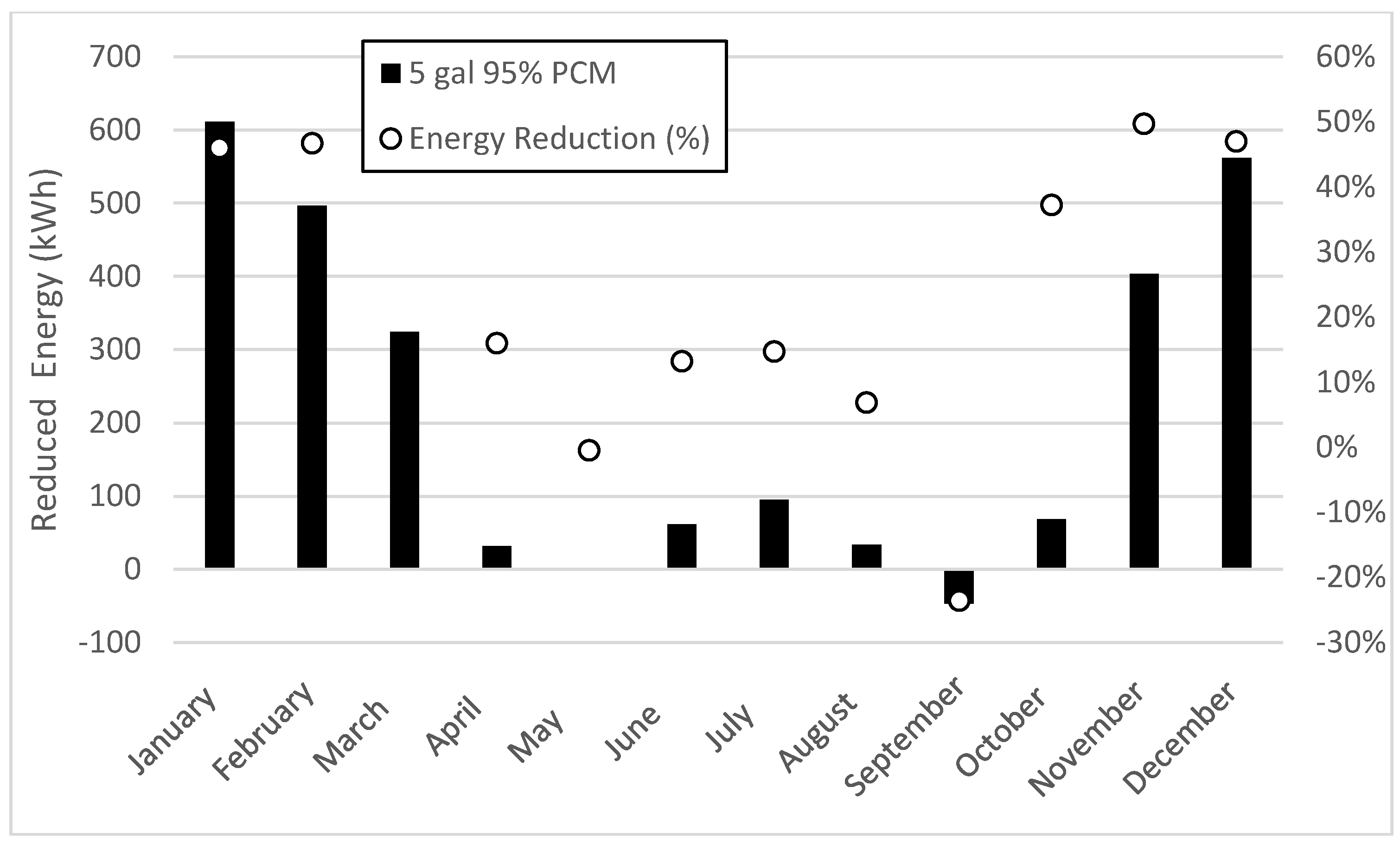
Simulations based on the equations presented in Section 3 were used to obtain the monthly energy requirements for each case. The total cooling and heating loads were numerically integrated using TRNSYS Type 46. This was the primary metric that was used to determine the energy reduction benefits of the ITC/TSM system. A month-by-month case was used for showing seasonal benefits as opposed to an overall yearly benefit. Although energy was added to the building during the heating months and extracted during the cooling months, energy is shown only as positive values in Figure 7 and Figure 8. April, May, and September had the magnitudes of the added and extracted energy summed together. This was because both the heating and cooling modes are likely to be active during these months.
The main objective of this study is to show the viability of tank volume reduction without loss of energy savings by implementing PCM. Simulations were completed for a 50-gallon tank without PCM, and a five-gallon tank with 95% of the volume occupied by PCM. Due to the size restrictions, the 50-gallon tank was required to be either buried at 1-m depth or located outside the building exposed to ambient conditions, and the five-gallon tank was located inside the building.
Figure 7 shows the required energy for the reference case and two ITC/TSM cases. It illustrates how the addition of PCM allows for similar results with a volume reduction of 90%. It needs to be noted that the heat transfer losses to the ambient conditions are different for each case. Since the five-gallon tank is kept inside the building, heat transfer losses are less compared to the 50-gallon tank. Figure 7 also shows results for the 50-gallon tank when it is located outdoors.
Another benefit of using the small PCM tank is the ability for the tank to be located in a temperature environment that is close to the desired tank temperature, allowing for heat transfer to the ambient to be reduced.
The thermal losses for the indoor five-gallon tank is 99.58% less than the outdoor 50-gallon tank, and 99.54% less than the buried 50-gallon tank. For all of the cases, the tank was assumed to be well-insulated, and has the same tank loss coefficient of 3 kJ/h m2 K.
Figure 8 shows the monthly percent reduction in energy required by the heat pump. Energy reduction is not consistent, with an average heating reduction of 48% and an average cooling reduction of 3%. The month of May has no significant benefits, and September has moderate losses (24%). However, these losses are offset by the considerable savings found between November–March. The results indicate that it is possible that the valve operating conditions and the PCM parameters are more beneficial for cold months. Using different PCM and adjusting operating regimens for a specific season could show an increase in benefits. Specifically, water circulation currently operates on a monthly schedule when switching between the HEX and the solar panel for temperature regulation. More benefits could be found, or the losses in September could be reduced if a semi-predictive method was used on a weekly basis instead of using historical averages on a monthly basis. Although a 24% increase in consumption for September sounds significant, it is only 46 kWh, and is around 2% of the total required energy for the reference model during the cooling months. These new operating conditions could likely benefit other transitional months, as mild temperatures showed the least benefits from the system. Again, it must be noted that these mild months consume the least amount of energy. The overall yearly savings of the ITC/TSM model was about 35%, and the ITC/TSM with the PCM model was about 35.2%.
5. Conclusions
This study showed the capability of reducing the energy consumption of a small, lightweight, free-standing building due to air conditioning and heating units through a water loop system designed for ITC/TSM. PCM was added for the purpose of reducing the tank volume without a significant loss of energy savings. Tank volume reduction also allowed for reduced heat transfer loss as a result of indoor storage, although it was not the only factor for energy savings. Three different models were constructed for simulation: a reference case, an ITC/TSM case, and an ITC/TSM with PCM case. A 50-gallon tank was used in simulations for the ITC/TSM case, and a five-gallon tank was used for the ITC/TSM with PCM case. Although there was a 90% reduction of tank size, the PCM allowed for similar energy savings. The overall yearly savings of the ITC/TSM model were about 35%, and the savings of the ITC/TSM with PCM model were about 35.2%.
Although there was a slight loss in savings using the smaller tank, further development can possibly minimize this loss or provide additional benefits. A complete parameter study of the PCM could allow further energy savings, as was seen in preliminary simulations for the melting temperature. Future simulations will also include complex buildings with interior walls, doors, and additional windows to allow simulations that are a better representative of physical applications. Studies will also be conducted to determine the benefits associated with split flow operation and semi-predictive methods for heating and cooling the water. This would allow portions of the flow to circulate through the building, while the remaining flow could be heated or cooled for the building benefit. These new operating regimes could be found using Bayesian classification techniques to minimize air conditioning and heating operating times.
Author Contributions
All of the authors have contributed toward developing and implementing the ideas and concepts presented in the paper. All of the authors have collaborated to obtain the results and have been involved in preparing the manuscript.
Funding
This research received no external funding.
Conflicts of Interest
The authors declare no conflict of interest.
References
- U.S Department of Energy. Household Energy Use in Georgia. Energy Information Administration, Independent Statistics & Analysis. 2009. Available online: https://www.eia.gov/consumption/residential/reports/2009/state_briefs/pdf/ga.pdf (accessed on 5 April 2018).
- U.S Department of Energy. Georgia State Profile and Energy Estimates. Energy Information Administration, Independent Statistics & Analysis. 2018. Available online: https://www.eia.gov/state/data.php?sid=GA#ConsumptionExpenditures (accessed on 5 April 2018).
- Valladares-rendón, L.G.; Schmid, G.; Lo, S. Review on energy savings by solar control techniques and optimal building orientation for the strategic placement of façade shading systems. Energy Build. 2017, 140, 458–479. [Google Scholar] [CrossRef]
- Tyagi, V.V.; Buddhi, D. PCM thermal storage in buildings: A state of art. Renew. Sustain. Energy Rev. 2007, 11, 1146–1166. [Google Scholar] [CrossRef]
- Shaviv, E.; Yezioro, A.; Capeluto, I.G. Thermal mass and night ventilation as passive cooling design strategy. Renew. Energy 2001, 24, 445–452. [Google Scholar] [CrossRef]
- Vivian, J.; Zarrella, A.; Emmi, G.; de Carli, M. An evaluation of the suitability of lumped-capacitance models in calculating energy needs and thermal behaviour of buildings. Energy Build. 2017, 150, 447–465. [Google Scholar] [CrossRef]
- Antonopoulos, K.A.; Koronaki, E. Envelope and indoor thermal capacitance of buildings. Appl. Therm. Eng. 1999, 19, 743–756. [Google Scholar] [CrossRef]
- Reilly, A.; Kinnane, O. The impact of thermal mass on building energy consumption. Appl. Energy 2017, 198, 108–121. [Google Scholar] [CrossRef]
- Dominković, D.F.; Gianniou, P.; Münster, M.; Heller, A.; Rode, C. Utilizing thermal building mass for storage in district heating systems: Combined building level simulations and system level optimization. Energy 2018, 153, 946–966. [Google Scholar] [CrossRef]
- Sha, P.; Asadi, I. Concrete as a thermal mass material for building applications—A review. J. Build. Eng. 2018, 19, 14–25. [Google Scholar]
- Verbeke, S.; Audenaert, A. Thermal inertia in buildings: A review of impacts across climate and building use. Renew. Sustain. Energy Rev. 2018, 82, 2300–2318. [Google Scholar] [CrossRef]
- Aste, N.; Angelotti, A.; Buzzetti, M. The influence of the external walls thermal inertia on the energy performance of well insulated buildings. Energy Build. 2009, 41, 1181–1187. [Google Scholar] [CrossRef]
- Slee, B.; Parkinson, T.; Hyde, R. Can you have too much thermal mass? In Proceedings of the 47th International Conference of the Architectural Science Association, Hong Kong, China, 13–16 November 2013. [Google Scholar]
- Navarro, L.; de Gracia, A.; Colclough, S.; Browne, M.; McCormack, S.J.; Griffiths, P.; Cabeza, L.F. Thermal energy storage in building integrated thermal systems: A review. Part 1: Active storage systems. Renew. Energy 2016, 88, 526–547. [Google Scholar] [CrossRef]
- Whiffen, T.R.; Russell-Smith, G.; Riffat, S.B. Active thermal mass enhancement using phase change materials. Energy Build. 2016, 111, 1–11. [Google Scholar] [CrossRef] [Green Version]
- Carpenter, J.; Mago, P.J.; Luck, R.; Cho, H. Passive energy management through increased thermal capacitance. Energy Build. 2014, 75, 465–471. [Google Scholar] [CrossRef] [Green Version]
- Heier, J.; Bales, C.; Martin, V. Combining thermal energy storage with buildings—A review. Renew. Sustain. Energy Rev. 2015, 42, 1305–1325. [Google Scholar] [CrossRef]
- Kong, X.; Jie, P.; Yao, C.; Liu, Y. Experimental study on thermal performance of phase change material passive and active combined using for building application in winter. Appl. Energy 2017, 206, 293–302. [Google Scholar] [CrossRef]
- Wilson, M.; Luck, R.; Mago, P.J. A First-Order Study of Reduced Energy Consumption via Increased Thermal Capacitance with Thermal Storage Management in a Micro-Building. Energies 2015, 8, 12266–12282. [Google Scholar] [CrossRef] [Green Version]
- University of Wisconsin-Madison; Solar Energy Laboratory. TRNSYS, a Transient Simulation Program; University of Wisconsin-Madison: Madison, WI, USA, 1975. [Google Scholar]
- Ibáñez, M.; Lázaro, A.; Zalba, B.; Cabeza, L.F. An approach to the simulation of PCMs in building applications using TRNSYS. Appl. Therm. Eng. 2005, 25, 1796–1807. [Google Scholar] [CrossRef]
- Kuznik, F.; Virgone, J.; Johannes, K. Development and validation of a new TRNSYS type for the simulation of external building walls containing PCM. Energy Build. 2010, 42, 1004–1009. [Google Scholar] [CrossRef]
- Lu, S.; Zhao, Y.; Fang, K.; Li, Y.; Sun, P. Establishment and experimental verification of TRNSYS model for PCM floor coupled with solar water heating system. Energy Build. 2017, 140, 245–260. [Google Scholar] [CrossRef]
- McKenna, P.; Turner, W.J.N.; Finn, D.P. Geocooling with integrated PCM thermal energy storage in a commercial building. Energy 2018, 144, 865–876. [Google Scholar] [CrossRef]
- University of Wisconsin-Madison; Solar Energy Laboratory. Multi Zone Building Modeling with Type56 and TRNBuild; University of Wisconsin-Madison: Madison, WI, USA, 2012. [Google Scholar]
- Kusuda, T.; Achenbach, P.R. Earth Temperatures and Thermal Diffusivity at Selected Stations in the United States. ASHRAE Trans. 1965, 71, 61–74. [Google Scholar]
- ASHRAE. ANSI/ASHRAE Standard 62.1-2010. Ventilation for Acceptable Indoor Air Quality; ASHRAE: Atlanta, GA, USA, 2010. [Google Scholar]
- Voller, V.R. An overview of numerical methods for solving phase change problems. Adv. Numer. Heat Transf. 1997, 1, 341–375. [Google Scholar]
- University of Wisconsin-Madison; Solar Energy Laboratory. Mathematical Reference; University of Wisconsin-Madison: Madison, WI, USA, 2004. [Google Scholar]
- Advanced Cooling Technologies. Phase Change Material (PCM) Selection. 2018. Available online: https://www.1-act.com/pcmselection/ (accessed on 5 April 2018).
- Solar Ratings and Certification Corporation. Certified Solar Collector; ICC-SRCC: Washington, DC, USA, 2012.
Figure 1.
Transient System Simulation Tool (TRNSYS) Schematic for Reference Building.

Figure 2.
TRNSYS schematic for the increased thermal capacitance (ITC)/thermal storage management (TSM) model.
Figure 2.
TRNSYS schematic for the increased thermal capacitance (ITC)/thermal storage management (TSM) model.

Figure 3.
Numerical Approximation of Specific Heat for Phase Change Materials (PCM).
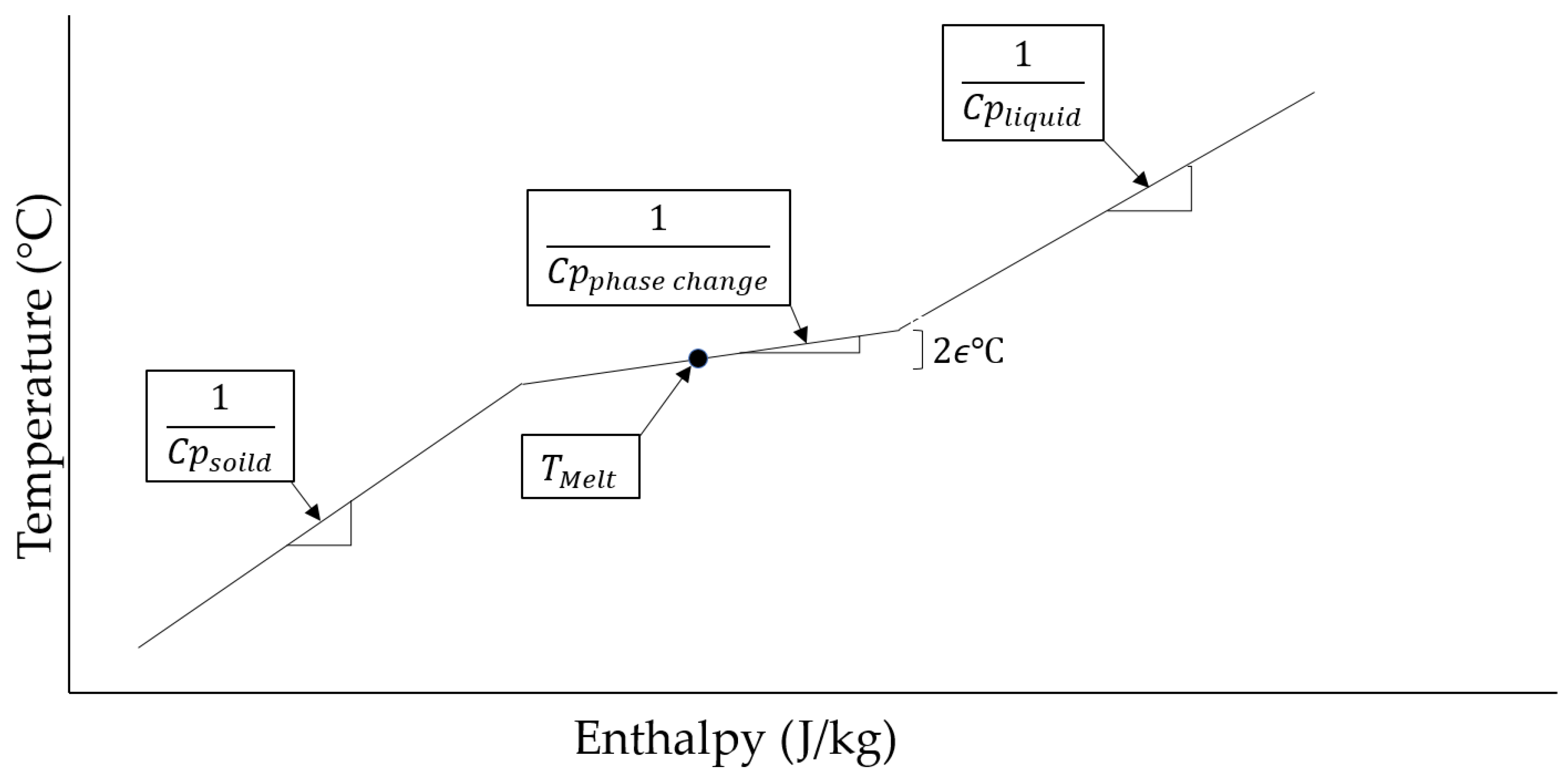
Figure 4.
Graphical Representation of Energy Flows into a Node.

Figure 5.
PCM Phase Change Operation.

Figure 6.
Building Free Response.

Figure 7.
Energy Consumption.
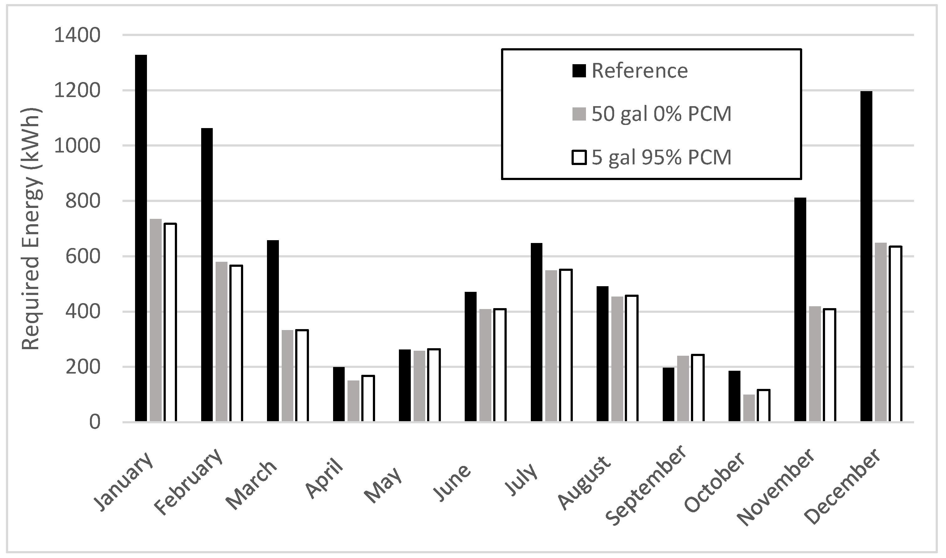
Figure 8.
Energy Reduction.

Table 1.
Building Materials and Properties.
| Surface Type | Layer (Inside to Outside) | Thickness (mm) | Conductivity (kJ/(h m K)) | Capacity (kJ/(kg K)) | Density (kg/m3) |
|---|---|---|---|---|---|
| External Wall | Plasterboard | 12 | 1.9 | 0.84 | 1200 |
| Fiberglass Insulation | 67 | 0.144 | 0.84 | 12 | |
| Wood Siding | 9 | 0.504 | 0.9 | 530 | |
| Floor | Tile | 25 | 5.17 | 1.5 | 880 |
| Insulation | 76 | 0.16 | 0.75 | 32 | |
| Concrete | 100 | 6.23 | 0.75 | 2242 | |
| Ceiling/Roof | Plasterboard | 10 | 1.9 | 0.84 | 1200 |
| Fiberglass Insulation | 112 | 0.144 | 0.84 | 12 | |
| Roof Decking | 19 | 0.504 | 0.9 | 530 |
Table 2.
Ground Coupling Properties.
| Ground Coupling Properties | Value |
|---|---|
| Tmean | 16.33 °C |
| Tamp | 4.945 °C |
| d | 0.12 m |
| α | 0.84 kJ/(kg K)) |
| tshift | 0 day |
Table 3.
Heat Pump Parameters.
| Heat Pump Parameter | Value |
|---|---|
| Rated Cooling Capacity | 10 kW (~3 ton) |
| Rated Heating Capacity | 10 kW |
| Rated Air Flowrate | 36 m3/min (1200 CFM) |
Table 4.
Heat Pump Nominal Thermostat Settings.
| Setpoint | Cooling (1 April to 31 October) | Heating (1 November to 31 March) |
|---|---|---|
| Daytime (8 a.m.–8 p.m.) | 22 °C | 20 °C |
| Evening (8 p.m.–8 a.m.) | 21 °C | 22 °C |
Table 5.
Tank Circulation Regime. HEX: heat exchanger.
| Season | Building Circulation | HEX Circulation | Solar Panel Circulation |
|---|---|---|---|
| Cooling Season | TTank ≤ TBuilding | TTank > TBuilding and TTank > TAmbient | N/A |
| Heating Season | TTank ≥ TBuilding | N/A | TTank < TBuilding and Collector is gaining energy 1 |
1 where TTank is the average tank temperature, TBuilding is the average building temperature, and TAmbient is the outdoor dry bulb temperature of Atlanta, Georgia.
Table 6.
PCM Parameters.
| PCM Parameter | Value |
|---|---|
| Heat of Fusion | 230 kJ/kg |
| Specific Heat | 2 kJ/kg K |
| Density (solid) | 900 kg/m3 |
| Melting Temperature | 21.5 °C |
Table 7.
Solar Panel Parameters for Solar Rating and Certification Corporation (SRCC) Data Sheet.
| Solar Panel Parameter | Value |
|---|---|
| Collector Area | 2 m2 |
| Intercept Efficiency | 0.775 |
| First Order Efficiency Coefficient | 18.37 kJ/(h m2 K) |
| Tested Flowrate per Unit Area | 70 kg/(h m2) |
| First Order Incidence Angle Modifier ( IAM) Coefficient | 0.0664 |
© 2018 by the authors. Licensee MDPI, Basel, Switzerland. This article is an open access article distributed under the terms and conditions of the Creative Commons Attribution (CC BY) license (http://creativecommons.org/licenses/by/4.0/).
Share and Cite
MDPI and ACS Style
Wilson, M.; Luck, R.; Mago, P.J.; Cho, H. Building Energy Management Using Increased Thermal Capacitance and Thermal Storage Management. Buildings 2018, 8, 86. https://doi.org/10.3390/buildings8070086
AMA Style
Wilson M, Luck R, Mago PJ, Cho H. Building Energy Management Using Increased Thermal Capacitance and Thermal Storage Management. Buildings. 2018; 8(7):86. https://doi.org/10.3390/buildings8070086
Chicago/Turabian StyleWilson, Mary, Rogelio Luck, Pedro J. Mago, and Heejin Cho. 2018. "Building Energy Management Using Increased Thermal Capacitance and Thermal Storage Management" Buildings 8, no. 7: 86. https://doi.org/10.3390/buildings8070086
Note that from the first issue of 2016, this journal uses article numbers instead of page numbers. See further details here.