Analytic Hierarchy Process & Multi Attribute Utility Theory Based Approach for the Selection of Lighting Systems in Residential Buildings: A Case Study

Abstract

This paper presents an approach developed for selecting lighting systems in residential buildings using an Analytic Hierarchy Process (AHP) and the Multi Criteria Decision Making Technique (MCDMT). The developed approach considers four selection criteria of lighting systems: life-cycle cost, illumination, environmental performance, and life-span. The criteria of selection, along with the most widely used lighting systems in residential buildings, were determined through questionnaire surveys with suppliers, maintenance managers, and lighting experts. The Analytic Hierarchy Process and Multi Attribute Utility Theory were utilized to assess the significant influence of the identified main and sub-criteria on the selection process, from the design point of view. The developed approach was tested on a real case project in selecting the lighting system for aresidential building in Saudi Arabia. The obtained results show that the life-cycle cost and illumination proprieties, followed by the service life were found to be the most influential measures in the selection process. The results also show that Light-Emitting Diode(LED) lighting systems prove to bear the highest initial cost while sustaining the best overall performance.

1. Introduction and Objective of the Work

Lightingisoneof themost importantof allbuilding systems; it impacts the buildings occupants’ visual comfort and behavior. Also, it has a high potential for energy efficiency and emission reduction. In Saudi Arabia, lighting represents a considerable portion of electricity consumption in residential buildings [1]. It contributes up to 50% of the total electricity consumption, and considerableCO₂ emissions [1,2]. In China for example, the power consumption due tolighting is estimated to account for approximately 13% of the total [3]. Lighting fixturesarealso identified as one of the main causes of extra energy consumption [4]. Thus, selecting an efficient lighting system design, or replacing existing one, is a crucial and a complex process for decision makers. The complexity is attributed to the consideration of multi criteria in the selection process.

In current practice, the selection process requires the involvement of a higher management level to resolve conflicts among project teams, and to make decisions based on experience rather than on scientific methodology, or on tools which may compromise the criteria and optimize the selection.

Furthermore, identifying the criteria of selection, along with the assessment of its importance, is the most important task in the selection process, andmay take long time to complete. The delay in finalizing the selection of a lighting system forongoing projects can cause cost-effective projects to waste time and money. Delays and/or cost overruns affect business portfolios, since theyleads to delays in other activities, and cause disruptions inthe projects globally.

The selection of a new lighting system, or replacing an old one, is usually carried out based on personal experience, and is therefore not subject to the needs and constraints that actually govern the selection of the best system based on the evaluation of performance against certain measures.

The literature reveals that over the years, a wide range of methods and techniques havebeen introduced to facilitate the selection process where multi criteria of selections are considered. There are several studies in the literature for selecting lighting systems in buildings. Most of these studies have focused on technical aspects of the selection, such as efficiency, safety, visual comfort, satisfaction, and energy consumption, etc. e.g., [3,5,6].

Since its introduction in 1980s, AHP alone, or combined with other techniques, has beenextensively utilized to facilitate the selection process in many complex applications in the building industry. AHP divides a complicated problem into a simple and manageable hierarchy of factors [3]. For example, in selecting lighting systems, [7] proposed an AHP-based framework which consists of various criteria for the installation of the median barriers for national highways. The selection criteria considered in the study were regional equity, safety, efficient economy, and installation possibilities, while giving high priority to safety. Lv et al. [3] also introduced an AHP-based evaluation system for an efficient lighting project. The system accounts for public policies combined with evaluation factors and sub factors. The considered factors were technology, equity, adequacy, economy, and environment. The system was tested in China’s energy conservation project. The results provided by the system showed that there were environmental benefits of 80% savings in energy consumption,a reduction of 10.98 billion tons of carbon emissions, and savings of up to 1.362 billion RMB.

Jin et al. [7] conducted a field study for measuring and evaluating the quality of interior lighting in shopping centers in China. The study considered visual comfort and users’ satisfaction. The study utilized a questionnaire to investigate the differences in people’s subjective evaluations. The findings of the study can be used by the designers to come up with a design that offers the most benefits for shopping mall shoppers.

Despenica et al. [8] looked at the problem of designing lighting systems in office buildings in different ways. The study considered the preference profiles of users by: (1) offering several choices in the same zone to avoid conflict; (2) allocating different zones among different profiles that may face conflict; and (3) measuring the tolerance and the lighting control behavior of the users.

In addition to AHP, simulation based models were also introduced in the literature to compare the use of Light-Emitting Diode (LED) and Compact Fluorescent Lamps (CFL). Energy consumption and greenhouse gas emissions from each alterative were calculated and compared, and then the best alternative was selected [9]. It is worth noting that the outputs of simulations allow for conducting IF THEN-type analyses. This assists decision makers to review different scenarios in the selection process. Although simulation-based models have been identified for their strength in analyzing multifaceted problems, the vital limitations of applying such methods in general are: (1) simulationsaretime-consuming technique, and require the collection of considerable amounts of data that may not be available in some situations, such as those in the facilities management industry; (2) They require the input of experts to offset the lack of data availability; (3) Simulations require dedicated professionals, which may be beyond the capabilities of some decision makers; and (4) Simulations require several runs to produce reliable outcomes.

Maleetipwan-Mattsson et al. [10] studied the factors that may affect the optimal lighting use in hospitals, and may lead to reductions in energy consumption. The study was conducted through measurements of the rooms, observations, and a questionnaire. Das et al. [11] introduced a model for the light design for the exterior, to meet energy and consumer demands by optimizing cost, increasing robustness, and by delivering reliable and high-quality exterior lighting. An LED flood lighting system was suggested for exterior lighting to achieve efficient lumen output.

Linhart and Scartezzini [12] carried out a comparison of two energy efficient lighting scenarios for evening lighting in offices buildings;the reference scenario had 4.5 W/m² of Lighting Power Density (LPD), and the test scenario, which wasmore energy efficient,had3.9 W/m² of LPD. The comparison was performed to extract the results of visual performance, visual comfort, and energy efficiency for evening lighting selection in office buildings. The results indicated that energy efficient lighting with 5 W/m²LPD can be easily achievable without degrading fair visual performance and comfort, such that can be obtained withlowerconnected lighting power.

Kelly and Rosenberg [13] conducted an intensive study onthe use of CFLs and LEDs in residential buildings in the US. Information from the past 25 years showed that CFLs faced many adoption barriers in the 1980s, due to consumer dissatisfaction and poor marketing strategies that were overcome by the US Department of Energy (DOE) and ENERGY STAR in 1999–2001. Although LEDs also faced certain market barriers in the past due to quality, cost, and functionality, soon after they gained popularity through efficient marketing strategies and DOE efforts to initiate CALiPER programs for technology advancements. The results showed that CFLs took longer to penetrate the market compared to LEDs, due to the lack of technological advancements and marketing efforts.

The main limitations of the above-described studies, individually or collectively, are that they did not adequately consider other important factors that may affect the selection process, such as life-cycle cost, light loss factor, land lumen depreciation, luminaire dirt depreciation, correlated color temperature (CCT), color rendering index (CRI), lumen (LM), and carbon dioxide (CO₂) emissions. In addition, the studies did not systematically integrate the opinions of the experts in the selection process, in the absence of the numerical data.

The objective of this paper is to present a systematic approach developed for selecting lighting systems in residential buildings. The approach addresses the aforementioned limitations incurrent practices, and to be applied by decision makers specializing in this type of work.

2. Overview of the Proposed Approach

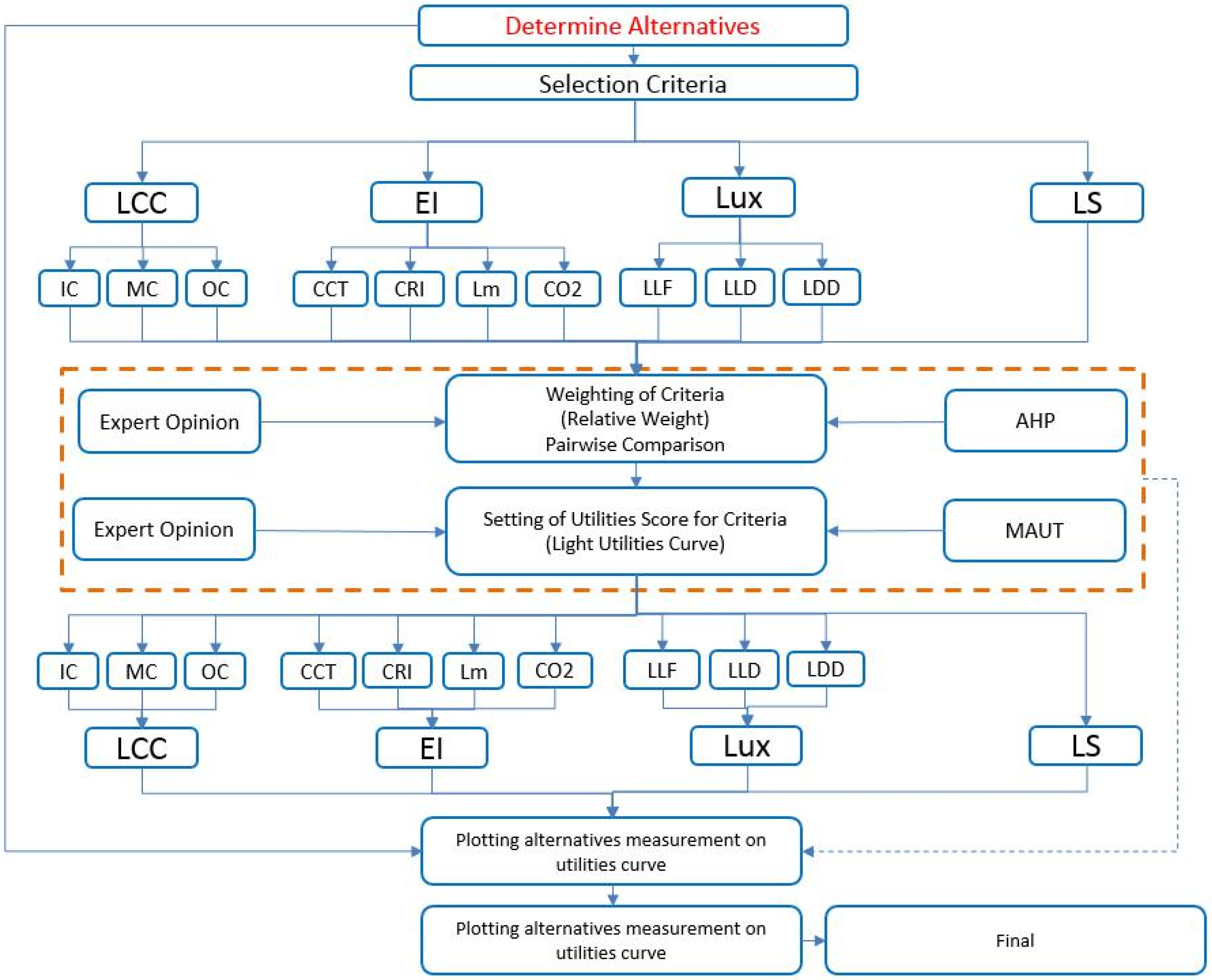
To meet the objective of this work, five principal stages were focused up, as shown in Figure 1. The first stage requires the identification of the most widely used alternatives forlighting systems in residential buildings in Saudi Arabia. In this stage, local project managers and suppliers in the private sector were consulted to determine the alternatives. The identified alternatives considered in this study are LEDs, CFLs, Incandescents, and Halogens.

The second stage involves the identification of the main and sub-criteria that should be considered in the selection process. This stage was carried out by conducting a pilot study with several local experts, mainly project managers, architects, and contractors. The identified main and sub-criteria are:(1) Life-cycle cost criterion, including initial, maintenance, and operating costs; (2) Environmental performance criterion, including correlated color temperature (CCT), color rendering index (CRI), lumen (LM), and carbon dioxide emissions; (3) Illumination criterion, including light loss factor, and land lumen depreciation; and (4) Luminaire dirt depreciation.

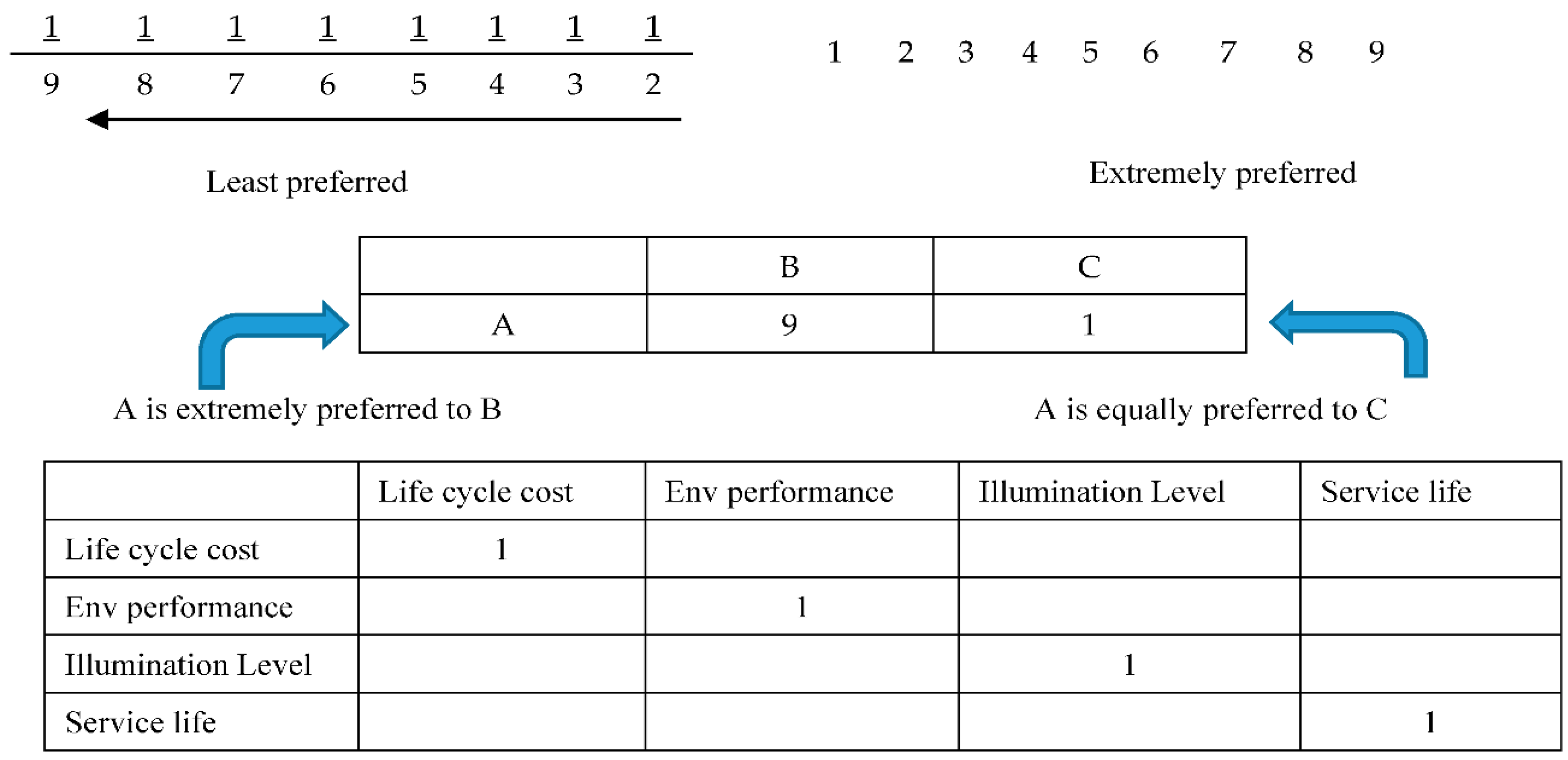
The third stage comprises the evaluation of the importance of the identified criteria by experts and decision makers using the AHP technique. The evaluation of criteria at this stage was performed using the pair-wise comparison matrix method, as shown in Figure 2. For example, the experts were asked to determine the level of importance through acomparison of the life-cycle cost criterion with all other criteria one by one, such as environmental performance, illumination level, and service life.

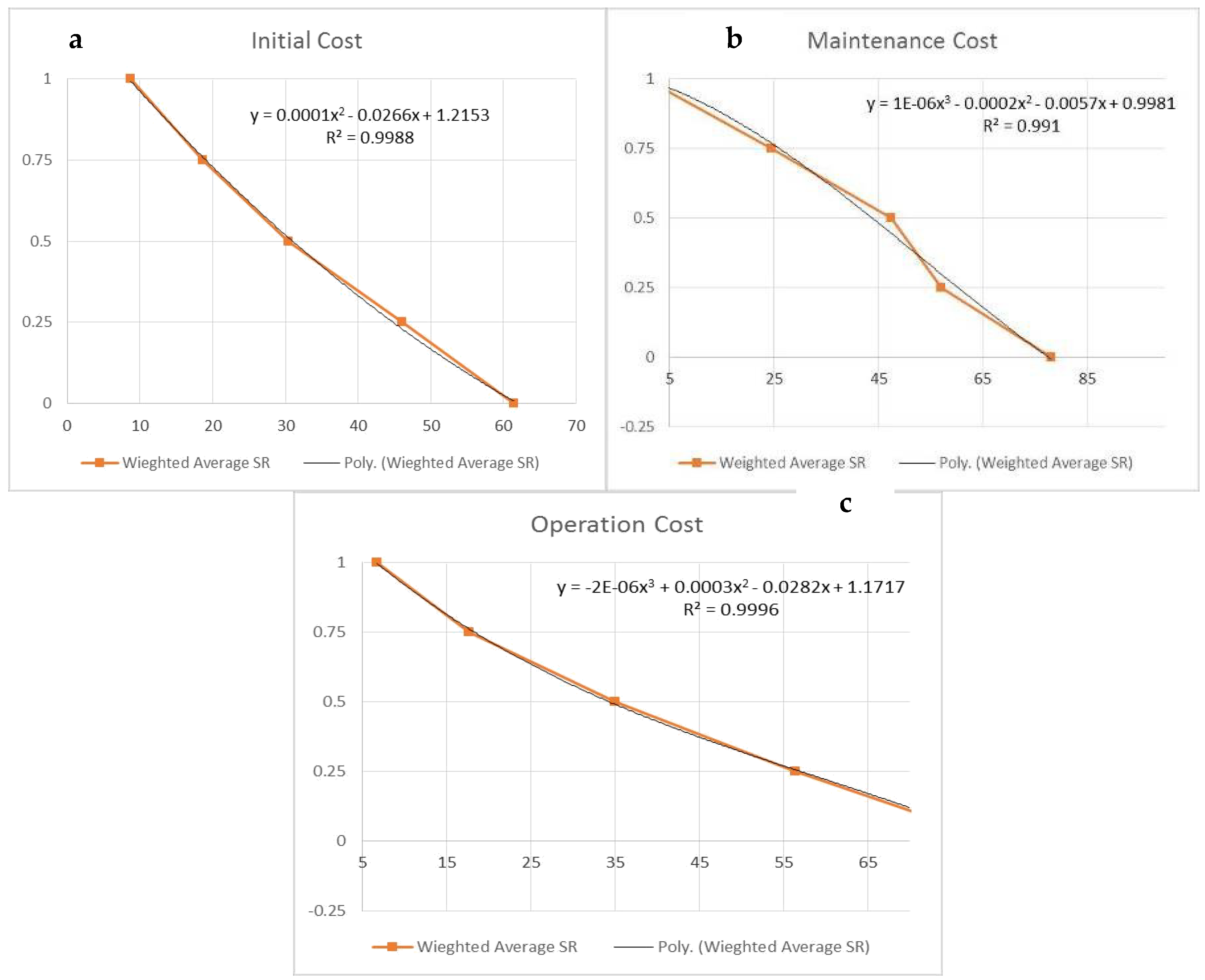
The fourth stage involves the development of the multi-utility theory curves, based on standards or expert opinions. For example, the Life-cycle cost criterion is divided into three sub-criteria, including initial cost, operating cost, and maintenance cost. The utility curves were built for all sub-criteria. For instance, in the initial cost criterion, the average of the best cost value was determined to be 8 Saudi Riyal (SR), while the highest average cost was 63 SR. Fifteen experts participated in developing these curves.

The incorporation of AHP and Multi Attribute Utility Theory (MAUT) occurs in the next step, in which each identified alternative measurement is plotted on all of the utility curves. In this stage, the performance of each alternative is measured over all the selected criteria. For instance, a compact florescent system has a service life of about 8000 h, and its annual operating cost is about 20.1 SR, while the LED has a service life of 25,000 h, and annual electricity costsare about 12 SR.

The final stage comprises the calculation of the total score, and the selection of the best system. The calculation of the performance of each alternative in each criterion was first measured using utility curves. The performance of each alternative was then multiplied by the importance of each criterion, as determined by AHP technique. The total score of each alternative was calculated by adding up its whole performance overall according to the selection criteria. Finally, the selection of the best alternative was done based on the highest obtained score in comparison to those of thealternatives.

2.1. Application of AHP and MAUT

Unlike with current methods, the developed approach combines AHP and MAUT to identify the significant influence of the identified main and sub-criteria in selecting lighting systems for residential buildings from a design point of view. Combining AHP and MAUT is relatively new in the selection process of complex problems e.g., [14]. AHP and MAUT are utilized to develop the proposed approach by applying the two techniques, based on experts’ opinions, across the community services organizations in the third and fourth stages described above.

In the third stage, AHP and MAUT are used to develop the selection method by measuring the importance of the main identified criteria: Life-Cycle Costs (LCC), environmental performance, illumination and life span. The evaluation process is extended to the sub-criteria to measure the importance of each sub-criterion, and to identify their impact on the main criterion, as well as the overall criteria. Both main and sub-criterion are given a relative weight through the AHP matrix and a pairwise comparison.

In the fourth stage, utility curves are developed for the criteria using experts’ judgments, by using the overall result with simple averages for the scale. The performance of alternatives in each main and sub-criteria are plotted against the developed curves with the measured scores. Lastly, the total scores are computed for all alternatives by having the grade for each, a comparison is carried out for the alternatives, and the highest obtained score is then selected. The following section explains these stages in more detail.

2.2. AHP and Pair-Wise Comparison

To be concise in taking a decision, a pair-wise comparison is conducted for main and sub selection criteria using AHP. The comparison is executed based on experts’ opinions, with relative importance applied to all categories and sub-categories. A scale of 1/9-9 is used, as illustrated in Figure 2. In the pair-wise comparison matrix, the experts first used the AHP decision-making technique to fill out the matrix. A quantification of relative weights is performed through this method for specific criteria set related to the priorities scale ratio of 1/9 (least preferred to most). The criteria in the first row and the first column must be compared to each other by the experts. The first matrix evaluates the main criteria, including LCC, environmental performance, illumination, and service life.

A quantification of relative weights are also performed through this method for specific criteria and its sub set, related to the priorities scale ratio of 1/9.

Table 1. Life-cycle cost.

Criteria	Initial Cost	Operation Cost	Maintenance Cost
Initial Cost	1	9	1
Operation Cost	Weight Criteria	1	1/9
Maintenance Cost	Weight Criteria	Weight Criteria	1

shows that initial cost is muchpreferred to operating cost (9 scores), while initial cost is equally preferred to maintenance cost (1 score). Each sub-selection criterion is evaluated for each main criterion, such as life-cycle cost, which includes initial, operating, and maintenance costs.

2.3. Measuring the Performance of the Identified Alternativesusing MAUT

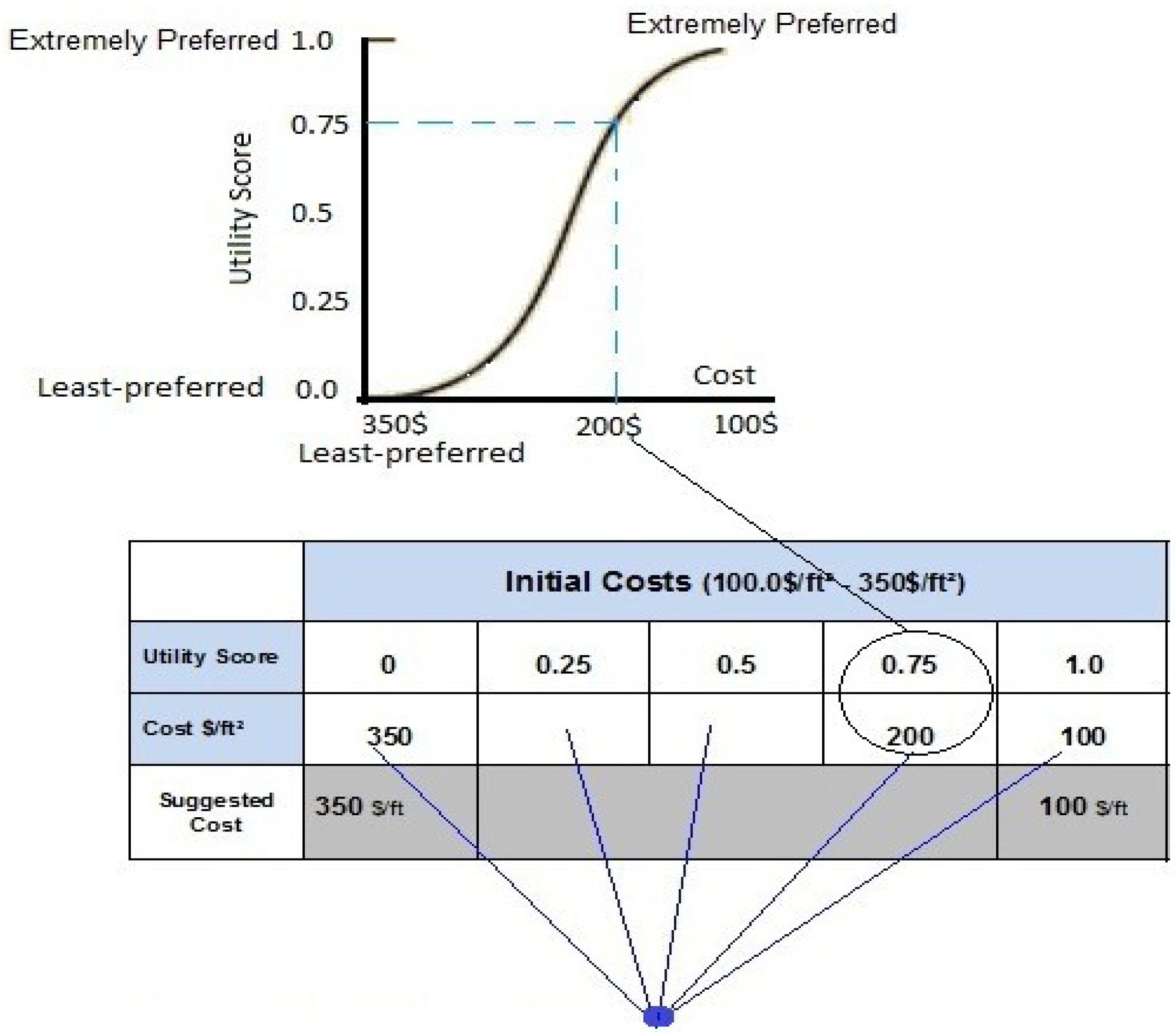
The Multi-Attribute Utility Technique (MAUT) is utilized to measure the performance of the identified alternatives against main and sub-criteria standardized values throughout the utility scores. This measurement is performed on the accepted responses to questionnaires, using the consistency and reliability measures. Ranking the criteria is done by measuring the weight of each criterion using pair-wise comparison and the AHP technique.

The MAUT method requires the determination of the highest and lowest value for each criterion. A utility score of 1.0 is assigned to the most-preferred value, while 0.0 is assigned to a least-preferred value. A midpoint value, which has a utility score of 0.5 is then identified by the experts. The midpoint value is a halfway value between the most- and least-preferred values [13,14]. After the identification of the midpoint value, ‘quarter point’ value, having a utility score of 0.25, is identified by the experts, which is a halfway value between the midpoint and least preferred values. Finally, a value function having a utility score of 0.75 is identified by the experts, which is a halfway value between most preferred and the midpoint value [15,16]. Once the experts determine these five values, a utility attribute or value function graph is plotted, as illustrated in Figure 3.

3. Data Collection, Analysis and Evaluation

3.1. Data Collection

The data required to carry out this study wascollected from three sources. The first source was local suppliers and technical reports. The collected data is used for the identification of lighting system alternatives which are widely used in residential buildings in Saudi Arabia. The identified alternatives are incandescent lamps, CFLs, and LED lamps. The second source was local experts, decision makers, and professionals from the private sectors, through a distributed survey over the business area. The data collected from this source is needed for the selection of alternatives, and it is utilized as a base reference for the analysis. The Third source is the experts’ opinion across the community services organization. The collected data from this source is used for measuring the importance of the identified main criteria using AHP and MAUT. It should be noted that the evaluation process was extended to the sub-criteria to measure the importance of each sub-criterion and its impact on the main criterion, as well as the overall criteria. The utility curves are also developed for the criteria using the collected information from experts’ judgments, by finding the overall result with simple averages for the scale.

3.2. Preliminary Survey

A pilot study was carried out in the form of a hard copy, and was distributed to the engineering support group. The survey was a significant tool that helped in improving the quality and efficiency of the survey prior to sharing it all across the community services. Important comments and changes were received from the experts, such as having the luminance specification compared to international standards, and the environmental performance due to CO₂release and other issues.

3.3. Main Survey

Hard copies and a softcopy were distributed to six departments of community services in Saudi Aramco, to the facilities, building proponents, design, and procurement engineers in the eastern, southern, and central regions. Eighteen responses were received and analyzed. In addition, hard copies and a softcopy were distributed to six community service departments in Saudi Aramco in the eastern, southern, and central regions, to collect as much information as possible. Thirteen responses were personally gathered from engineers, supervisors, and building service coordinators.

3.4. Data Analysis and Evaluation

Total scores are calculated for the alternatives using a statistical method to make comparisons balanced, in terms of the weight of importance. Then, values were ranked to determine the best or the highest score alternative as the preferred selection. This was calculated using the following mathematical equations:

$$Vi\left(x\right)=\sum W_i{U}_i= \left(W_{Lcc}{U}_{Lcc}\right)+(W_{Env}{U}_{Env})+\left(W_{Lm}{U}_{Lm}\right)+\left(W_{Ls}{U}_{Ls}\right)$$

(1)

$$W_{Lcc}{U}_{Lcc}=(W_{Ic}{U}_{Ic})+(W_{Mc}{U}_{Mc})+(W_{Oc}{U}_{Oc})$$

(2)

$$W_{Env}{U}_{Env}=\left(W_{Cct}{U}_{Cct}\right)+\left(W_{Cri}{U}_{Cri}\right)+\left(W_{Co2}{U}_{Co2}\right)+\left(W_{Lm/w}{U}_{Lm/w}\right)$$

(3)

$$W_{Lm}{U}_{Lm}=\left(W_{Llf}{U}_{Llf}\right)+\left(W_{Lld}{U}_{Lld}\right)+\left(W_{Ldd}{U}_{Ldd}\right)$$

(4)

4. Case Project

To investigate the applicability of the developed approach in selecting an efficient lighting system for residential buildings in Saudi Arabia, a case project for Saudi Aramco is tested. Four different lighting systems were considered: LED, CFL, Incandescent, and Halogen. The approach considers four main criteria: life-cycle cost, illumination, environmental performance, and life span.

Table 2. Lamp data and Specifications of considered lighting systems.

	Lamp Data
Type	LED(Home) Daylight	Compact Fluorescent (CFL)	Quartz Halogen	Incandescent	Unit
Number	1	1	1	1	-
Hours/year	8765	8765	8765	8765	-
Lumens	800	950	885	890	-
Lamp Life(hours)	25000	8000	2000	1000	-
Efficacy	100	63.3	17	14.8	-
Efficiency	14.64%	9.27%	2.49%	2.17%	-
Operating Costs
Electricity per year	12.00	20.96	72.96	84.16	-
Bulbs per year	<1	1	4	9	-
Total cost per year	9.94	17.61	45.81	61.54	-
Energy and Environmental Information
kWh used per year	75	131	456	526	-
CO2	104	184 (0.09)	637	735 (0.37)	-
released/year	(0.05)	-	(0.32)	-	pounds (tons)
SO2released/year.	1	2	7	8	pounds
NOx released/year	1	1	4	5	pounds
Mercury released/year	1	1	4	5	ounces
Coal used	35 lbs.	62 lbs.	214 lbs.	247 lbs.	-
Emissions Equivalents
Same as driving	85	150	519	599	miles
Trees needed	1	1	2	2	-

presents the specifications and the data for the four alternatives, including quotesgathered from vendors. The energy, operation, and maintenance costs are computed considering the wattage used, as presented in

Table 3. Obtained alternatives values.

Criteria	LED	CFL	Halogen	Incandescent
Initial Cost (SR/EA)	50	25	15	10
	30	15	15	5
Average	40	10	15	10
	40	16.66	15	8.333
	30.58	45	80	115
Main. Cost SR	25	40	75	110
	20	30	90	127
Average	23.52	38.585	83.33	119.04
Oper. SR/Year	12	20.96	72.96	84.16
	14	28	60	80
	10	20	65	90
Average	12	22.986	65.98	84.72
	3000	4000	3000	2700
CCT Temp K	5000	2700	3000	2700
	4000	6000	2700	3000
Average	4000	4233	2900	2800
	80	80	100	100
CRI Unity	94	82	100	90
	90	82	100	85
Average	88	81.33	100	91.666
	93.49	63.56	17.011	14.83
Lumen/Watt	84	65.625	17.14	13.3
	120	61	16.03	18
Average	99.164	63.39	16.73	15.37
	0.05	0.09	0.32	0.37
CO2 Tons	0.1	0.1	0.3	0.4
	0.08	0.08	0.25	0.33
Average	0.076	0.09	0.29	0.366
	100	80	80	80
LLF %	98	90	70	70
	70	85	85	80
Average	89.33	85	78.33	76.66
	85	95	85	80
LLD %	93	80	80	85
	90	75	70	80
Average	89.33	83.33	78.33	81.66
	80	86	70	86
LDD %	93	88	88	80
	78	70	90	75
Average	83.66	81.33	82.66	80.33
	50,000	8000	2000	1000
Hours	10,000	10,000	4000	1250
	25,000	15,000	3000	1250
Average	28,333	11,000	3000	1166

. As mentioned earlier, to apply the developed approach, the decision makers needed to fill in the matrix, as shown in Figure 2.

4.1. Analysis of One Response

Fifteen responses from experts were received.

Table 4. AHP Main criteria for respondents.

Criteria	Life-cycle Cost	Environment Performance	Illumination Level	Service Life
Life-cycle Cost	1	3	1	2
Envi. Performance	0.333333333	1	1	0.33
Illumination Level	1	1	1	3
Service Life	0.5	3	0.333333333	1
Total	2.833333333	8	3.333333333	6.333333333

shows the selection criteria pair-wise comparison matrix filled out by one of the fifteen received responses, while

Table 5. AHP Normalization for main criteria matrix.

Normalization
Life-cycle Cost	0.353	0.375	0.300	0.316
Envi. Performance	0.118	0.125	0.300	0.053
Illumination Level	0.353	0.125	0.300	0.474
Service Life	0.176	0.375	0.100	0.158
Total	1.000	1.000	1.000	1.000

represents AHP normalization for the main criteria Matrix of that response.

Table 6. Relative weights.

Geometric Mean(1)	Average(2)	Aw(3)	Lamda(4)	CI(5)	CR(6)
0.341	0.336	1.499981	4.465123	0.151214	0.168015
0.130	0.14882	0.641151	4.308239	-	-
0.293	0.312906	1.404683	4.489147	-	-
0.236	0.202341	0.921069	4.552054	-	-
1	1	1.116721	4.453641	-	-

contains the following information: column (1) shows the calculated geometric mean for row values in pair-wise comparison matrix. Column (2) contains relative weights (Eigen-value) of criteria that are equal to the geometric mean of the same criteria over the sum of all criterion’s geometric mean. Column (3) represents the criteria’s vector weight that is equal to the sum of multiplication of values in each matrix row and relative weights. Column (4) consists of λ_max values that wereobtained through the division of vector weight by the relative weight of each criterion. Columns (5) and (6) show the results of the consistency ratio thatwereobtained by dividing the consistency index (CI) with the value of the random consistency index (RCI), as shown in Equation (5):

CR = CI/RCI

(5)

The CI value is computed as (CI = (λmax − n)/ (n − 1)), while the Random inconsistency index(RI) value calculated through size n matrix from

Table 7. Random inconsistency index (R.I).

RI	0.00	0.00	0.58	0.90	1.12	1.24	1.32	1.41	1.45	1.49	1.51	1.48
n	1	2	3	4	5	6	7	8	9	10	11	12

. Inconsistency in the judgment matrix may occur when CR surpasses 0.10; then, the judgment of the experts will be unacceptable, while few of the responses are ignored because of their high consistency ratio.

4.2. Analysis of Responses

As mentioned earlier, fifteen responses were gathered with Cr values of between 0.1 to 0.15, as presented in

Table 8. Summarization for main criteria.

AHP	Selection Criteria	LCC	Env. Imp	Illumination	Life Services	Selection Criteria
Relative weight	1	0.335932	0.14881965	0.3129063	0.202341331	1
	2	0.412573	0.13918128	0.301462	0.146783626	1
	3	0.220959	0.25252525	0.2058081	0.320707071	1
	4	0.347342	0.05686400	0.3632515	0.232542155	1
	5	0.322156	0.09301779	0.3911223	0.193703045	1
	6	0.490335	0.07542089	0.2364662	0.197777904	1
	7	0.403257	0.31675546	0.1142163	0.165770341	1
	8	0.465753	0.07951440	0.29443	0.160301788	1
	9	0.335317	0.13640873	0.2867063	0.24156746	1
	10	0.419480	0.24805194	0.1954545	0.137012987	1
	11	0.524155	0.06831951	0.2810906	0.126434949	1
	12	0.518764	0.13066361	0.2580664	0.092505721	1
	13	0.362540	0.11968954	0.2802288	0.23754085	1
	14	0.389437	0.08091204	0.1796863	0.349963986	1
	15	0.410669	0.09738005	0.2659407	0.226010101	1
	Median	0.403257	0.11968954	0.2802288	0.197777904	1.0009541
	Mean	0.397620	0.13520086	0.2654416	0.201796326	1.0000596
	Mode	0.403257	0.11968954	0.2802288	0.197777904	1.0009541
	SD	0.078857	0.07465856	0.0685367	0.067552084	0.2896044
	Var	0.005829	0.00522553	0.0044037	0.004278079	0.0838707
	∑Var	0.0197371	-	-	-	-
	Cα	0.8739113	-	-	-	-

. The relative weights for the selection criteria were computed using the AHP technique, with the help of mean values. Statistical analyses were conducted on the data to calculate the mean, median, mode, standard deviation, variance, and Carbanches alpha. As depicted in Table 8, the average result for the calculated weights are as follows: 0.3976 for the LCC, 0.135 for environmental performance, 0.2654 for the luminaire and 0.201 for the life span. The Cα is 0.87, which indicates the responses are reliable.

As shown in

Table 9. Summarization for sub criteria of 15 respondents.

Indicator	Selection Criteria				Total
LCC	IC	OC	M&R C	-	-
Mean	0.42873544	0.412597228	0.1586673	-	1
Cα	0.733				-
Env	CCT	CRI	Illuminance	CO2	-
Mean	0.34814605	0.196111953	0.3811138	0.074628217	1
Cα	0.83530522				-
Luminaire	Light Loss factor	Lamp Lumen Depr.	Luminaire Dirt Depr.	-	-
Mean	0.58870629	0.262042989	0.1492507	-	1
Cα	0.74479691				-

, the sub-criteria of LCC may be summarized as follows: 42.87% for the IC, 41.25% for Operating Costs (OC) and 15.28% for the M&R cost. The Cα is 0.733, which indicates that the considered responses are reliable. As the sub-criteria of the environment, the average results for the calculated weights wereas follows: 34.8% for the CCT, 19.6% for CRI, 38.11 for luminance and 7% for CO₂ Release. The Cα is 0.833, which indicates that the considered responses are reliable. As for the Illumination components, the average result for the calculated weights are shown as follows: 58.87% for the LLF, 26.2% for the Lamp Lumen Depreciation (LLD) and 14.9 % for LDD. The Cα is 0.74479691, which indicates that the considered responses are reliable.

4.3. Reliability Analysis of Responses

Cronbach’s alpha was utilized and applied to examine the reliability of the expert’s opinion. This value is the coefficient of reliability, which examines the internal consistency of sample psychometric scores. This describes the effective measurement of the single unit dimensional latent construct by the set of variables. The coefficient is a function of observations that is equal to the ratio of the true variance to the total variance of measurement, and it is expressed through the following equation:

Cα:n/n − 1(1 − ∑Vi/V)

(6)

where, C alpha has value scaled from 0 to 1, and reliability is proportional to score and the acceptable range variance is from 0.7 to 1. The results presented in Table 8 and Table 9 show that the C. Alpha for main criteria is 0.87, while C alpha for the LCC, Environment, and Luminaire are 0.73, 0.83 and 0.74, respectively, which indicates that the considered responses are reliable.

4.4. Measurement of Preference Utility Values

The second section of the survey deals with the measurement of preference utility values for the selection criteria using MAUT technique. Adequate and favorable ranges of all weighted criteria utility scores were obtained by utilizing this technique, as explained in the previous section. The experts assign a preference value on a scale of 0 to 1.0 for each utility score for different criterion, leading to the selection of the most suitable lighting system. For instance, in the initial cost criterion, one expert determined the best value was 10 SR, while the worst was 80 SR, as shown in

Table 10. Summary of initial cost utilities score.

			Initial Cost
Utilities Score	0	0.25	0.5	0.75	1
Cost SR/EA	80	60	35	25	10
Suggested	80 SR	-	-	-	5 SR

. These assigned scores are gathered from different experts, and their averages are used to construct the utility curves for various selection criteria, as presented in

Table 11. Initial cost utility scores for all respondents.

CTQ’S	SR	SR	Initial Cost	SR	SR
1	50	35	10	3	1
2	60	50	20	15	10
3	65	55	40	7.5	5
4	80	60	40	20	10
5	60	40	30	15	5
6	75	40	30	20	10
7	70	50	40	30	15
8	55	30	25	20	15
9	60	50	30	25	10
10	40	25	15	10	5
11	60	50	30	20	10
12	40	35	15	10	5
13	80	60	35	25	10
14	60	35	25	15	5
15	100	80	60	30	15
Utilities sores	0	0.25	0.5	0.75	1

(initial cost utility scores). The developed utility curves include life-cycle costs, environmental performance, illumination, and life span; all variables are constructed in the same way.

Table 11 represents the judgments of 15 experts of the initial cost based on their needs and experiences with utilities score, which range from (zero, 0.25, 0.5, 0.75, and 1). Average values were then calculated to develop the utility curves, as noted in Figure 4, Figure 5 and Figure 6. The initial cost is represented in Figure 4a, with best curve fitting of a second-degree equation.This equation indicating that the utility score is directly proportional to cost, and the acceptable average cost range is between (8.73 SR–63 SR).

The maintenance cost is represented in Figure 4b, with abest curve fitting of third degree equation. This equation indicates that the utility score is directly proportional to cost, and that the acceptable average cost range is between (1.73 SR–77.3 SR). The operation cost is represented in Figure 4c with a best curve fitting of third degree equation. This equation indicates that the utility score is directly proportional to cost, and the acceptable average cost range is between (8.46 SR–76.66 SR).

The CCT is represented in Figure 5a, with best curve fitting of third degree equation. This equation indicates that the utility score is directly proportional to the correlated color temperature, ranging between (2700–5700 k). The CRI is represented in Figure 5b, with best curve fitting of the 1st-degree equation. It indicates that the utility score is directly proportional to color rendering index ranging between (80.3–98.2). The luminance is represented in Figure 5c, with best curve fitting of the first-degree equation. This indicates that the utility score is directly proportional to luminance ranging between (17.8–97.33 lumen). The CO₂ release is represented in Figure 5d, with best curve fitting of the third-degree equation. It indicates that the utility score is directly proportional to Carbon Dioxide ranging between (0.045–1.133 Ton).

The LLF is represented in Figure 6a with best curve fitting of second-degree equation. It indicates that the utility score is directly proportional with a light loss factor ranging between (68.67–98.33%). The LLD is represented in Figure 6d with best curve fitting of second-degree equation. This indicates that the utility score is directly proportional to lamp lumen depreciation ranging between (73.33–99.06%). The LDD is represented in Figure 6c with best curve fitting of third-degree equation. It indicates that the utility score is directly proportional to lamp dirt depreciation ranging between (83–98.93%). The life span is represented in Figure 6b with best curve fitting of third-degree equation. This indicates that the utility score is directly proportional to life span ranging between (3800–77,333 Hrs).

5. Discussion and Selection of Alternatives

Table 12. Alternatives utilities score AVG.

Criteria	LED	CFL	Halogen	Incandescent
IC	0.311	0.799444444	0.8385	1
MC	0.76628237	0.537836178	0	0
OC	0.873044	0.657700349	0.0425045	0
CCT	0.8851	0.98597	0.31277	0.24766
CRI	0.4059	0.059233333	1	0.596566667
Lm/Watt	1	0.628627099	0.0126431	0
CO2	0.9495173	0.923516602	0.6316291	0.558957837
LLF %	0.6898	0.5442	0.3422	0.295866667
LLD %	0.59371111	0.363511111	0.2101778	0.308511111
LDD %	1	1	1	1
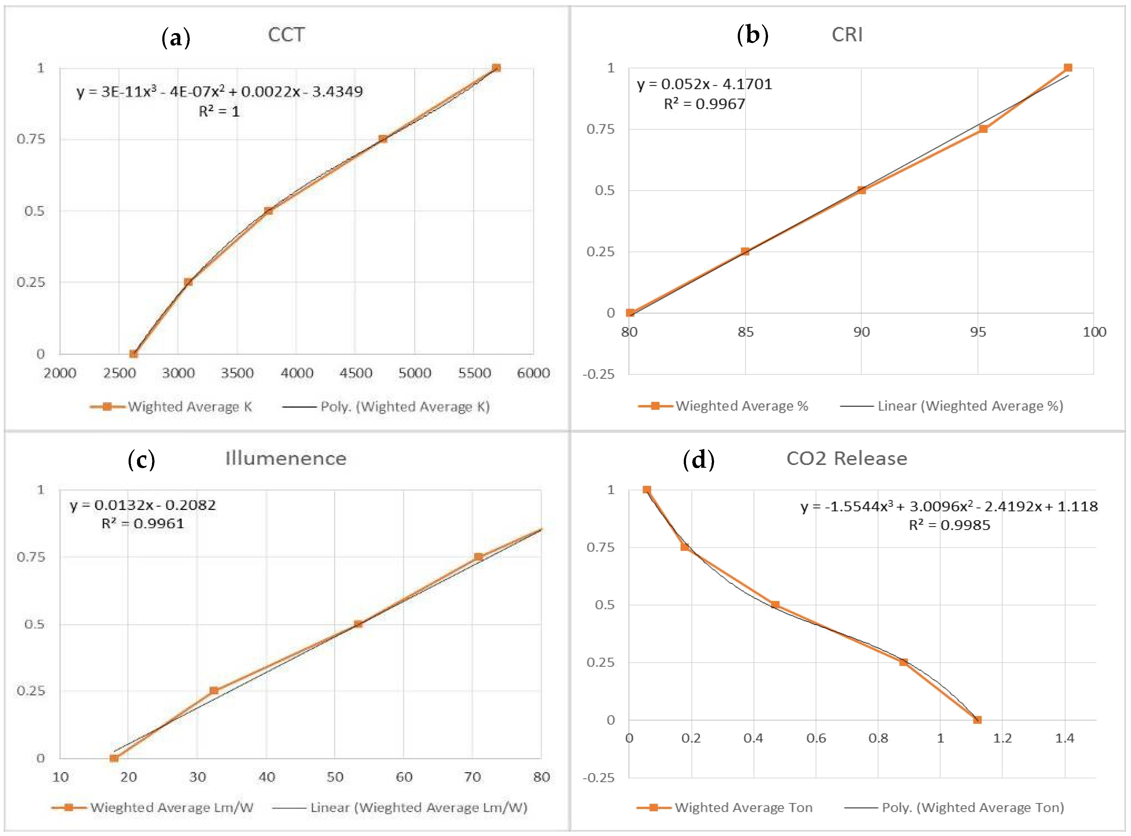
Hrs	0.62674815	0.256824	0	0

represents the scoring of the considered alternatives and their contributions against the measurement curve, for both main and sub-criteria with values and utility scores. These values can be approached by applying themmanually, using the utility curve, or subjecting themto the derived equations of the developed curves, as presented in Figure 6. Multiplying the values in Table 12 by the obtained relative weights of criteria using AHPs Matrix in

Table 13. Importance weights for criteria.

Pair-Wise Matrix	Criteria	Relative Weight (Importance Weight)
Relative weights By AHP	IC	0.4287354
	MC	0.1586673
	OC	0.4125972
	CCT	0.3481460
	CRI	0.1961119
	Lm/Watt	0.3811138
	CO2	0.0746282
	LLF %	0.5887062
	LLD %	0.2620429
	LDD %	0.14925072
	Hrs	0.20179632

resulted in the obtained score for all alternatives, as presented in

Table 14. Obtained score by each alternative overall criteria.

MAUT	Criteria	LED	CFL	Halogen	Incandescent
Weights(Utility Expert)	IC	0.13333672	0.342750164	0.359494665	0.428735438
	MC	0.31616598	0.221909716	0.00	0.00
	OC	0.13852356	0.104355561	0.00674407	0.00
	CCT	0.30814407	0.343261563	0.108889641	0.086221851
	CRI	0.07960184	0.011616365	0.196111953	0.116993854
	Lm/Watt	0.38111378	0.239578448	0.004818458	0.00
	CO2	0.07086078	0.068920397	0.047137353	0.041714027
	LLF %	0.4060896	0.320373964	0.201455293	0.174178568
	LLD %	0.15557783	0.095255538	0.055075613	0.080843174
	LDD %	0.14925072	0.149250719	0.149250719	0.149250719
	Hrs	0.12647547	0.05182614	0.00	0.00

. For example, the performance (utility value) of LED in initial cost criterion is 0.311, as presented in Table 12, while the importance weight (relative weight) of the initial cost is 0.428, as presented in Table 13. Multiplying the utility value (0.311) by the relative weight (0.428) is equal to 0.133, as presented in Table 14.

Figure 7 presents the alternatives’ performance overall according to the sub-criteria. It shows that the best alternative in initial cost is Incandescent followed by Halogen, due to their low prices compared to LEDs. In contrast, LED system proved to have the best performance with the lowest maintenance and operation costs, followed by CFL.

The LED also proved to have the best performance in many sub-criteria, such as CO₂emissions, light loss factor LLF, lumen land depreciation, and the overall service life.

The total score of each alternative was calculated by adding up its globalperformance overall, according to the selection criteria, using Equation (1). Finally, the selection of the best alternative is made based on the highest obtained score in comparison to the other alternatives.

Table 15. Total obtained scores for various alternatives (Total Grade).

Weight-Major Criteria	Alternative	LCC	Env. Performance	Illuminance	Life Span	Total Score
	LED	0.23381152	0.11353093	0.1887072	0.126475474	0.662525
	CFL	0.26601451	0.08968911	0.1499427	0.05182614	0.557472
	Halogen	0.14562417	0.048260948	0.1077113	0	0.301596
	Incandescent	0.17047416	0.03311471	0.1073107	0	0.3109

presents the total computed scores for all alternatives overall, according to the main criteria. The highest score value was recorded for the LED, followed by CFL. The LED obtains a total score of 0.66, and 0.56 for the CFL, as noted in the table. Hence, the best lighting system to be used in residential buildings according to the tested criteria is the LED system, followed by CFL.

6. Conclusions

The main purpose of this study is to develop an approach that assists decision makers and buildings proponents or owners in selecting the best lighting system for residential buildings based upon economic, environmental, illumination, and life span criteria. AHP and MAUT are integrated into this study to evaluate the importance of the various selection criteria and different lighting alternatives. The integration of both techniques assist in converting different units of measurement into a unified system, in order to the appropriate parties to make informed decisions.

The application of the developed approach on a case project of selecting lighting system showed that the life-cycle cost criterion is proven to have the highest importance weight of 40%, followed by illumination with 26%, and service life with 20%. The case project proved that the initial cost is not the only criterion that should be taken into account. The provided results also showed that the LED lighting system was recorded to have the worst performance, and a high impact on initial costs, while it was proven to have the best overall performance for selection criteria. The present work can be extended to include other criteria, such as visual comfort and user satisfaction, and to account for uncertainties associated with LCC and expert opinions. The study is limited to residential projects, which are themselves subject to many constraints. The methodology can be applied in selecting the lighting system for office buildings after determining the selection criteria, which may differ from those of residential buildings.

References

1. Bertoldi, P.; Atanasiu, B. Characterization of residential lighting consumption in the Enlarged European Union and policies to save energy. Int. J. Green Energy 2008, 5, 15–34. [Google Scholar] [CrossRef]
2. Muhamad, W.; Zain, M.; AbWahab, N.; AbdKadir, R. Energy efficient lighting system design for building. In Proceedings of the International Conference on Intelligent Systems, Modelling and Simulation, Liverpool, UK, 27–29 January 2010. [Google Scholar]
3. Lv, F.; Wang, Z.; Ding, Y.; Li, Y.; Zhu, N. A systematic method for evaluating the effects of efficient lighting projects in China. Energy Effic. 2016, 9, 1037–1052. [Google Scholar] [CrossRef]
4. Na, R.; Lin, S.; Shen, Z.; Gu, L. Case study of quantifying energy loss through ceiling-attic recessed lighting fixtures through 3D numerical simulation. J. Arch. Eng. 2017, 23. [Google Scholar] [CrossRef]
5. Belcher, B.M.C.; Klein, A.K.; Gadberry, B. User survey of subjective preference for street lightings sources. J. Arch. Eng. 1999, 5, 92–97. [Google Scholar] [CrossRef]
6. Atanasiu, B.; Bertoldi, P. Residential electricity consumption in new Member states and candidate countries. Energy Build. 2018, 40, 112–125. [Google Scholar] [CrossRef]
7. Jin, H.; Li, X.; Kang, J.; Kong, Z. An evaluation of the lighting environment in the public space of shopping centres. Build. Environ. 2017, 115, 228–235. [Google Scholar] [CrossRef]
8. Despenic, M.; Chraibi, S.; Lashina, T.; Rosemann, A. Lighting preference profiles of users in an open office environment. Build. Environ. 2017, 116, 89–107. [Google Scholar] [CrossRef]
9. Cao, J.; Choi, C.; Zhao, F. Agent-based modelling of the adoption of high-efficiency lighting in the residential sector. Sustain. Energy Technol. Assess. 2017, 19, 70–78. [Google Scholar]
10. Maleetipwan-Mattsson, P.; Laike, T.; Johansson, M. Factors affecting optimal lighting use in shared hospital environments: A case study. Build. Environ. 2016, 96, 260–269. [Google Scholar] [CrossRef]
11. Das, N.; Pal, N.; Pradip, S.K. Economic cost analysis of LED over HPS flood lights for an efficient exterior lighting design using solar PV. Build. Environ. 2015, 89, 380–392. [Google Scholar] [CrossRef]
12. Linhart, F.; Scartezzini, J.L. Evening office lighting—Visual comfort vs. energy efficiency vs. performance? Build. Environ. 2011, 46, 981–989. [Google Scholar] [CrossRef]
13. Kelly, K.; Rosenberg, M. Some Light Reading: Understanding Trends Residential CFL and LED Adoption. ACEEE Summer Study on Energy Efficiency in Buildings. 2016. Available online: www.aceee.org (accessed on 12 February 2018).
14. Doczy, R.; AbdelRazig, Y. Green buildings case study analysis using AHP and MAUT in sustainability and costs. J. Arch. Eng. 2017. [Google Scholar] [CrossRef]
15. Alshamrani, O. Evaluation of School Buildings Using LCC & Sustainability Measures—Selection of Structure & Envelope Types for Schools—Sustainable School Buildings vs. Conventional School Buildings; LAP LAMBERT Academic Publishing: Saarbrucken, Germany, 2014. [Google Scholar]
16. Alshamrani, O.; Alkass, S.; Galal, K. Evaluation of LCC and sustainability criteria for school buildings in Canada using AHP and MAUT. In Proceedings of the 4rd International/Construction Specialty Conference, 11th Canadian Society of Civil Engineering Conference, Montreal, QC, Canada, 4–5 May 2010. [Google Scholar]
Figure 1. Model’s methodology.
Buildings 08 00073 g001
Figure 2. AHP scale and matrix.
Buildings 08 00073 g002
Figure 3. Function/utility attribute graph.
Buildings 08 00073 g003
Figure 4. Utilities curves of (a) initial, (b) maintenance, and (c) operating costs.
Buildings 08 00073 g004
Figure 5. Utilities curves of (a) CCT, (b) CRI, (c) luminance, and (d) CO2 release.
Buildings 08 00073 g005
Figure 6. Utilities curves of (a) LLF, (b) service life, (c) LDD, and (d) LLD.
Buildings 08 00073 g006
Figure 7. Alternatives performance overall selection criteria.
Buildings 08 00073 g007