Optimizing Single-Ply Low-Slope Roofing Assemblies for Insulation Value

1
Building and Roofing Science, GAF, 1 Campus Drive, Parsippany, NJ 07054, USA
2
Product Management, GAF, 1 Campus Drive, Parsippany, NJ 07054, USA
*
Author to whom correspondence should be addressed.
Buildings 2018, 8(5), 64; https://doi.org/10.3390/buildings8050064
Submission received: 22 March 2018
/
Revised: 23 April 2018
/
Accepted: 26 April 2018
/
Published: 28 April 2018
Abstract
:Low-slope roofing assemblies can be designed with a range of insulation and membrane-attachment methods. Various building and energy codes appear to assume fastening methods to have an insignificant effect on insulation value, meaning that design and effective values are essentially the same. Recent studies showing that mechanically fastened systems could have very significant loss of insulation value are reviewed. This study uses thermal losses shown in those recent studies and examines the practical effect on various roof assemblies. Fully mechanically attached systems are compared with those that use adhesive attachment for the membrane and part of the insulation assembly. The thermal losses are shown to be significant and are presented in terms of the economic loss of the insulation. The cost of lost R-value is contrasted with the cost of attachment. A system based on a first layer of mechanically attached insulation with a second layer of insulation and membrane being adhered is shown to be very similar in cost, once the lost R-value is included. Finally, the loss in energy efficiency is calculated over a 15-year time frame. When total system costs include fastening as well as energy efficiency, then mechanically attached systems are essentially equivalent to some fully adhered approaches. Overall, the work challenges the code assumption that fastening methods do not significantly impact insulation efficiency. Furthermore, the results have implications for any analysis that considers such factors as carbon footprint, since building-energy efficiencies might be lower than currently assumed.
1. Introduction
The journey towards more energy-efficient commercial buildings has generally involved reducing heat energy flow across or through various components of the building envelope. Thus, windows have been made more insulating as well as more reflective, especially in the infrared regions of the energy spectrum. Similarly, roof systems have incorporated greater thicknesses of insulation, dictated by increasing code requirements. The introduction of thermoplastic roof membranes, starting with polyvinyl chloride (PVC) in the 1960s followed by thermoplastic polyolefin (TPO) in the 1990s, marked the beginning of an accelerating trend towards reflective roofing. Together, these highly reflective membranes now account for about 50% of the US roofing market.
Architects and building designers have many specification options available that can assist in improving the energy efficiency of the building envelope, including thermal insulation, infrared-specific filter coatings on windows, and reflective roof membranes. However, as with many such efforts there can be a law of diminishing returns. While many individual building components have a prescriptive minimum thermal resistance or insulation value (R-value, °F ft2.hr/Btu or RSI, m2 K/W) there is the question as to a system’s or an assembly’s total thermal transmittance (U-factor, or the inverse of thermal resistance). It is important to note that R-value and RSI, used throughout this work, refer to the thermal resistance of the material or entire assembly, depending on context, and not that of the interior surface.
This study considers the effective R-value of a common low-slope roofing assembly. Such roofs are generally considered to have a slope of less than 2:12 (9.46 degrees). The analysis was done for an assembly consisting of a steel deck, two layers of polyisocyanurate foam insulation (commonly referred to as polyiso or PIR), and a single-ply membrane. Examples of single-ply membranes include ethylene propylene diene monomer (EPDM), flexible PVC and TPO. The latter two membranes are typically white and highly reflective and are considered advantageous for their impact in terms of urban heat-island reduction and building energy-efficiency improvements [1,2,3]. Some assemblies included a high density (HD) polyiso board at the deck level. The goal was to evaluate differences between the design and effective thermal insulation values caused by various attachment methods commonly in use in the roofing industry. Design R-value refers to the R-value intended for the building or sub-component such as the roof assembly by the architect or other design professional. The effective R-value refers to the insulation value that is actually achieved after such practical matters as installation methods are taken into account. In this study, the impact of various methods of fastening a roof assembly are evaluated for their effect on the difference between the design R-value, intended by the architect, and the effective R-value achieved after actual construction.
2. Background
When specifying an insulation value for a low-slope system, designers rely on published material insulation values provided by the manufacturer. They may calculate the total system R-value by also taking into account the insulating value of cover boards, when used, and all other sub-components. Importantly, the International Energy Conservation Code (IECC) [4] and American Society of Heating, Refrigerating, and Air-Conditioning Engineers (ASHRAE) 90.1 state that insulation above deck must be continuous. ASHRAE 90.1 defines continuous insulation (ci) as “insulation that is uncompressed and continuous across all structural members without thermal bridges other than fasteners and service openings” [5].
A possible conclusion from ASHRAE’s ci definition is that thermal bridging due to fasteners is not significant or is unavoidable and, therefore, tolerated. An analysis by Burch, Shoback, and Cavanaugh found that metal fasteners reduced the overall thermal resistance of insulated metal deck assemblies from 3–8% depending on insulation thickness [6]. They used a finite difference model to analyze overall thermal resistance for assemblies using 50 fasteners per 100 square feet (5.38 per square meter). The results were in reasonable agreement with earlier work based on simpler estimation methods.
A more recent analysis of thermal bridging by Olson, Saldanha and Hsu used finite-element modeling to evaluate the impact of metal fasteners and other penetrations in a model single-ply system [7]. Their assembly comprised the following components, listed in ascending order:
- Interior air film;
- 22 ga corrugated steel deck;
- ½ in. (1.27 cm) thick gypsum board to serve as substrate for a vapor retarder (R 0.45) (RSI 0.080);
- 4.5 in. (11.4 cm) thick polyiso insulation, installed in two layers; insulation joints assumed to be staggered with no losses (R 25.2.) (RSI 4.43);
- Either ½ in. (1.27 cm) thick gypsum board (R 0.45) (RSI 0.080) or ½ in. (1.27 cm) thick polyiso cover board (R 2.5, RSI 0.44) depending on the model;
- Roofing membrane with insulation value of 0;
- Exterior air film.
Their analysis examined heat transfer in three zones of a model rectangular roof; field, corner and perimeter. Such zones have different fastener densities depending on wind uplift requirements related to location and building codes. Olson, Saldanha and Hsu based their analysis on a 19,200 ft2 (1784 m2) rectangular roof with fastener densities required to resist wind uplift according to Factory Mutual (FM) Class 1–90. The interior temperature was assumed to be 69.8 °F (21 °C) and an exterior ambient temperature of −0.4 °F (−18 °C). Such a roof was found to have reductions in R-value as compared to an assembly having zero fasteners as shown in Table 1.
The loss of R-value shown in Table 1 was calculated for fasteners that extended from above the cover board down through the steel deck. The area-weighted overall losses in effective insulation value shown were found to be 17% and 16% for gypsum and polysio cover boards, respectively.
Singh et al. carried out a very similar analysis again using finite-element modeling, but considered system U-factor (i.e., the overall coefficient of heat transfer, Btu/(hr ft2 °F) or W/(m2 K)) and modeled based on temperatures within three climate zones represented by Orlando, FL, Atlanta, GA, and St. Paul, MN, US [8]. They assumed a total roof area of 10,000 ft2 (929 m2) and higher overall fastener density compared to Olson et al. The reduction from designed R-value for a similar system to that of Olson et al. was found to be about 35%. For a roof zone having a fastener density of 1.0 /ft2 (10.78 /m2) Singh et al. calculated a loss from designed R-value of 32%, this comparing well with about 28% and 29% for the corner zone per Olson et al.
The modeled losses from designed R-value, per Olson et al. and Singh et al., are such that designers considering the mechanical attachment of insulation and a roof membrane should possibly consider large reductions in the assumed system R-value. Such reductions have implications for both building energy efficiency and the specification of heating, ventilation, and air conditioning (HVAC) systems. This study aims to examine alternative installation strategies based on adhesive attachments that reduce the loss of effective R-value. Loss of insulation value has an economic cost that was modeled and compared to the increased cost of alternate attachment methods. Replication of the prior work was out of the scope of this effort; the goal was to evaluate the reduction from designed R-value using the loss data previously obtained.
Another potential loss in building energy efficiency attributed to roof assembly design is caused by the billowing of mechanically attached single-ply membranes and consequent drawing up of conditioned air (e.g., infiltration). This has recently been extensively modeled by Pallin et al. [9], but is beyond the scope of this study.
3. General Description of the Roof Assemblies
The roof systems were based on three single-story buildings less than 35 feet (10.67 m) high. The largest was based on that of a so-called “big box” building, with a roof area of 125,000 ft2 (11,613 m2) in a rectangular configuration of approximately 290 × 431 ft (88.4 × 131.4 m). Two smaller buildings were also considered, with areas of 50,000 ft2 (4645 m2) and 15,000 ft2 (1394 m2), each with width-to-length ratios of 1:1.5. In every case, the roof was assumed to be a new installation, i.e., new construction or a total roof replacement. The zones of a roof assembly are as shown in Figure 1.
The mechanical attachment used #12 fasteners and 3 in. (7.6 cm) diameter plates throughout. Fastener patterns and densities were calculated based on a wind uplift requirement of 120 pounds per square foot (5.746 kPa), a 22 ga. (0.64 mm) metal deck, and a 60 mil (1.52 mm) single-ply thermoplastic membrane having a width of 10 feet (3.05 m). The roof assemblies, shown in order for each case considered, are described in Table 2.
Two membrane scenarios were used: a new membrane with an initial solar reflectance of 76 and emittance of 90, and a three-year aged reflectance of 68 and emittance of 83, the latter representing long-term roof performance. These values would be typical of a TPO membrane [10].
3.1. Description of the Membrane Attachment Methods
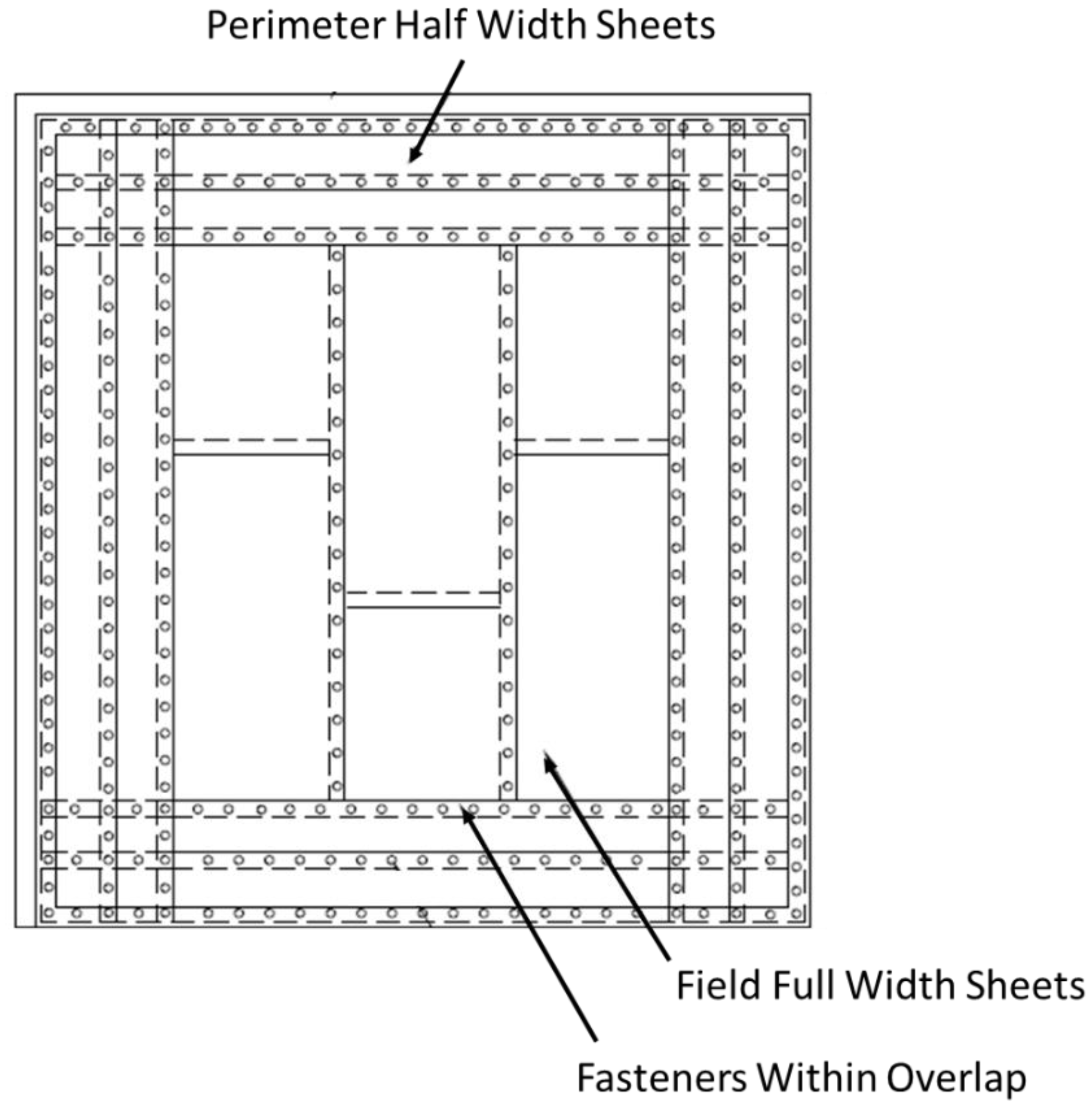
For Cases IA and IB, the membrane was mechanically attached using #12 (5.484 mm) fasteners and 3 in. (7.6 cm) diameter plates, installed 6 in. (15.24 cm) on center, as shown in Figure 2.
In Cases IIA and IIB, the plates are coated to enable induction welding of the membrane to the plates. For Cases III and IV, the membrane was attached to the top layer of insulation using a conventional adhesive designed for smooth, unbacked membranes.
3.2. Description of the Insulation Attachment Methods
In Cases IA and IB the insulation boards are attached using five fasteners through each of the topmost 4 × 8 ft. (122 × 244 cm) layer boards down through the steel deck.
Cases IA and IB are essentially identical except for the possibility of installing a vapor retarder on top of the first layer of 1/2 in. (1.27 cm) thick insulation in Case IB. In Cases IIA and IIB, the fasteners were applied through the topmost layer of insulation down through the steel deck. For Cases III and IV, the bottom insulation layer only was attached to the steel deck. All subsequent layers were adhered using conventional insulation adhesive.
The insulation fastener densities (e.g., use rates), per 4 × 8 ft. (122 × 244 cm) polyiso board, were identical for each building size, and are summarized in Table 3.
3.3. Total Fastener Densities and Loss of Effective R-Value
Taking into account both membrane and insulation fasteners, the overall roof fastener densities were calculated to be as shown in Table 4.
The work of Olson et al. was used as a basis for predicting loss of insulation value in this work. Their modeling focused on a single roof and provided changes in U-factor for three different fastener densities corresponding to the field, perimeter and corner zones. Their data was recalculated here as percent reduction from design R-value as a function of fastener density, with the resulting relationship being shown in Figure 3.
The relationship shown in Figure 3 was calculated to be y = 23.851x + 5.0192 (or y = 2.216x + 5.0192 when fastener density was expressed as #/m2).
4. Building Energy-Use Modeling
Petrie et al. used the simplified transient analysis of roofs model (STAR) [11,12] as the basis of the energy calculator tool known as CoolCalc, published by Oak Ridge National Laboratory (ORNL) [13]. The tool was developed to provide estimated energy cost differences associated with changing reflectivity and emissivity properties for roofing membranes and thermal insulation values. Subsequently, a modified version, CoolCalcPeak, was published that calculated savings when demand charges were factored in [14]. Demand charges are a cost per kilowatt at the highest level of demand during a specific billing period (e.g., 15 min) and are added to the total kilowatt per hour usage level in that period. The tool also enables the costs/savings associated with changing insulation levels to be calculated. The tools incorporate climate data for 263 US cities to establish outdoor temperatures. Indoor temperatures of 73 °F (23 °C) for summer and 70 °F (21 °C) are used as indoor boundary conditions.
CoolCalc and CoolCalcPeak make no assumption as to building geometry. They simply calculate energy loads on a building due to roof design (reflectance, emissivity and insulation values) and local climate factors. Those energy loads might be a large percentage of the total for a wide, low building, or a small percentage for a tall, narrow building. The calculators are estimating energy loads due to the roof alone. For this study, CoolCalcPeak was used throughout.
5. Model Input Data
According to the Department of Energy Buildings Energy Data Book, electricity is used to supply less than 20% of space heating energy demand for commercial buildings [15]. Therefore, natural gas was the assumed heat source for this study, with costs based on the annual average by state for commercial customers using 2016 US Energy Information Administration data [16]. Electricity costs were based on annual averages for 2016, for commercial customers by state, obtained from the US Energy Information Agency [17].
Demand charges were obtained per utility for each city being studied, from a Utility Rate Database [18]. Rates are checked and updated annually by the National Renewable Energy Laboratories, in partnership with Illinois State University’s Institute for Regulatory Policy Studies. In cases where multi-tiered demand charges were cited, these were averaged across the applicable months to provide the single input required by CoolCalcPeak.
The energy-cost data used is shown in Table 5. Electric demand charges were obtained for the cities being evaluated, based on medium-size commercial customers’ tariffs. Gas costs were the annual averages for 2016, for commercial customers by state
Although this study is, necessarily, limited to the use of the most recent published energy-cost information, projections to 2040 do not suggest significant changes. The Annual Energy Outlook 2017, U.S. Energy Information Administration, projects gas costs rising from 8 to 12 USD per thousand cubic feet (28.25 to 42.38 USD per hundred cubic meter) between 2016 and 2040 [19]. Similarly, average electric costs were projected to increase from 0.105 to 0.115 USD per kWhr across the same period.
The CoolCalcPeak calculator compares energy costs relative to a nominally non-reflective (e.g., dark absorptive) roof membrane. Two scenarios were used; an initial solar reflectance of 76 and emittance of 90 and a three-year aged reflectance of 68 and emittance of 83, these representing long-term roof performance. This would be typical of a thermoplastic membrane such as TPO. A design insulation value of R 30 (RSI 5.283) was used throughout, which was a conservative average from the 2015 International Energy Conservation Code.
The energy savings were first calculated using the design R-value and then for the effective R-value, each being calculated relative to a dark absorptive membrane per CoolCalcPeak. The difference between these two values represented the loss in energy efficiency due to the difference between design and effective R-values.
The building air-conditioning coefficient of performance was set as 2.5 and the natural gas heating efficiency was set as 0.8. Both are high-efficiency values and would be more typical of today’s heating and air-conditioning systems installed in new construction.
6. Results
This analysis evaluates the costs associated with a prescribed roof design based on R 30 and the resultant effective R-value due to attachment methodology. These costs are the lost economic value of R-value purchased but not achieved due to fastener thermal shortcircuits. Also, there is the cost of those fasteners and in the case of adhered systems, the adhesive cost. None of the costs include labor charges due to the difficulty of determining typical values. Labor costs vary significantly by location and by the approach taken by installers. For example, some contractors use a fixed crew size and vary the installation time while others use different size crews depending on the type of installation.
6.1. Loss of Insulation Value Due to Fasteners
Using the fastener densities shown in Table 4, together with the relationship between fastener density and percent reduction in R-value, the effective R-values are as shown in Table 6.
The percent reduction from designed insulation value is shown in Table 7, this being the effective values shown in Table 6 as a percent of the R-30 (RSI 5.283) design.
The effective R-values for each assembly and roof size are significantly lower than the design R-30 (RSI 5.283) in most cases, which questions the assumption that the insulation is effectively continuous. For Case III, which uses a ½ inch (1.27 cm) layer of mechanically attached polyiso with all subsequent layers being adhered, the reduction in insulation value was small. Note that the loss of insulation value is largest for Cases IA and IB, at about 15%. This is lower than the approximately 30% shown by Olson et al. and Singh et al., but for both studies the fastener densities corresponded to those used in the corners of mechanically attached assemblies. The results shown in Table 7 are representative of the entire roof assembly.
Examination of the effective insulation values shown in Table 7 indicates that the greatest percent reduction in R-value is for the smallest building size. This is due to the smaller roof areas having the largest percentage of perimeter and corner areas, with their associated higher fastener densities for mechanically fastened assemblies.
6.2. Loss of Installed Economic Value Due to Fasteners
The reduction from designed R-value, indicated in Table 6 and Table 7, has an immediate cost, i.e., the economic value of the “lost” insulation. This was calculated in terms of US dollars per R-value lost, i.e., purchased material that did not contribute to insulation, assuming that the installation costs would remain the same regardless of any difference between design and effective R-value. The costs are summarized in Table 8. For the standard polyiso boards, a material-based cost to the building owner of 0.10 USD per sq.ft per R-1 was assumed. For the ½ inch product used in Cases IB, IIB, and III, a material cost of 1.00 USD per sq. ft. per R-1 was assumed.
The insulation cost in lost R-value for a fully mechanically attached system is 56,057 USD for the 125,000 sq. ft. (11,613 m2) big box-type construction, as indicated in Table 8 for Case IA. This is a significant loss in economic value and Case IB is almost double that, due to the use of the ½ in. (1.27 cm) HD polyiso. This is also seen in a comparison of the costs for Case IIB with IIA. It should be noted that the loss in R-value for HD polyiso could be compensated for by its benefits, such as rigidity and compressive strength, and its ability to act as a base for a vapor retarder.
The lowest cost and most effective assembly in terms of R-value is Case IV. That assembly uses a first layer of mechanically attached 1 ½ in. (3.81 cm) polyiso which could act as a base for a vapor retarder. The remainder of the assembly is all adhered, including the top layer of HD polyiso. In general, it is clear that reductions in effective R-value due to fasteners are “expensive” for HD versus standard polyiso.
In addition to the cost of reduction from design to effective R-value, the mechanically attached assemblies have a higher fastener cost versus those that only mechanically attached the first insulation layer. In Table 9, the fastener cost is shown which takes into account fastener length (shorter being lower cost), added fastener plate for inductive attachment costs for Cases IIA and IIB, as well as fastener densities for each assembly.
6.3. Cost Due to Adhesive Use
For Cases III and IV, there is the added cost of adhesives. For the purposes of this analysis, two types of adhesive attachment were considered:
- Low-rise foam adhesive for adhering polyiso insulation to the substrate. This was used in Case III to attach the first layer of polyiso to the mechanically attached HD polyiso board and the second layer of polyiso insulation to the first. In Case IV, the low-rise foam adhesive adhered the second layer of polyiso insulation to the first. The cost of the adhesive was assumed to be 0.20 USD per square foot.
- A solvent-based adhesive for attaching the membrane to the substrate. This was assumed to cost 0.28 USD per square foot.
Thus, the adhesive costs are as shown in Table 10.
6.4. Total Material Costs Associated with System Attachment and Lost R-Value
The total costs involved in deviating from the design R 30, due to lost R-value caused by thermal shorts, and fastener and adhesive costs for each case and building size are shown in Figure 4, Figure 5 and Figure 6.
The lowest cost-deviation system is Case IIA for all building sizes, this being an inductive plate attachment. It is followed by Case IA, a conventional mechanically attached system. However, based solely on lost insulation value, Case IV is the preferred system for all building sizes. This is based on two layers of polyiso, the first being mechanically attached and each subsequent layer being adhered. Also, as noted previously, whenever HD polyiso is used there is a high cost associated with mechanically attaching it.
It is instructive to compare Case IA versus IV. As noted earlier, Case IA is widely regarded as the lowest-cost option for single-ply membrane installation. The calculations summarized in Figure 6 indeed show that the fastener costs in Case IA are far lower than the fastener and adhesive costs for Case IV. However, overall Case IA is higher in costs than is generally recognized due to the lost R-value. This lost R-value also has long-term implications due to energy-efficiency reduction, which is discussed next.
6.5. Loss of Energy Efficiency Due to Fasteners
The effective R-values shown in Table 6 were used to calculate the cost of a building’s reduced energy efficiency relative to the design R 30 (RSI 5.283) over a 15-year time frame. The latter was chosen based on the published R-values representing the time weighted 15-year long-term thermal resistance [20,21]. Given that reflective membranes lose some of their reflectivity over time, the three-year aged membrane data was used, with the results being summarized in Table 11.
A close examination of Table 11 suggests that the ORNL CoolCalcPeak model is causing some rounding discrepancies due to the sometimes small differences between R-design and R-effective. However, the data are believed to be directionally correct based on the overall trends.
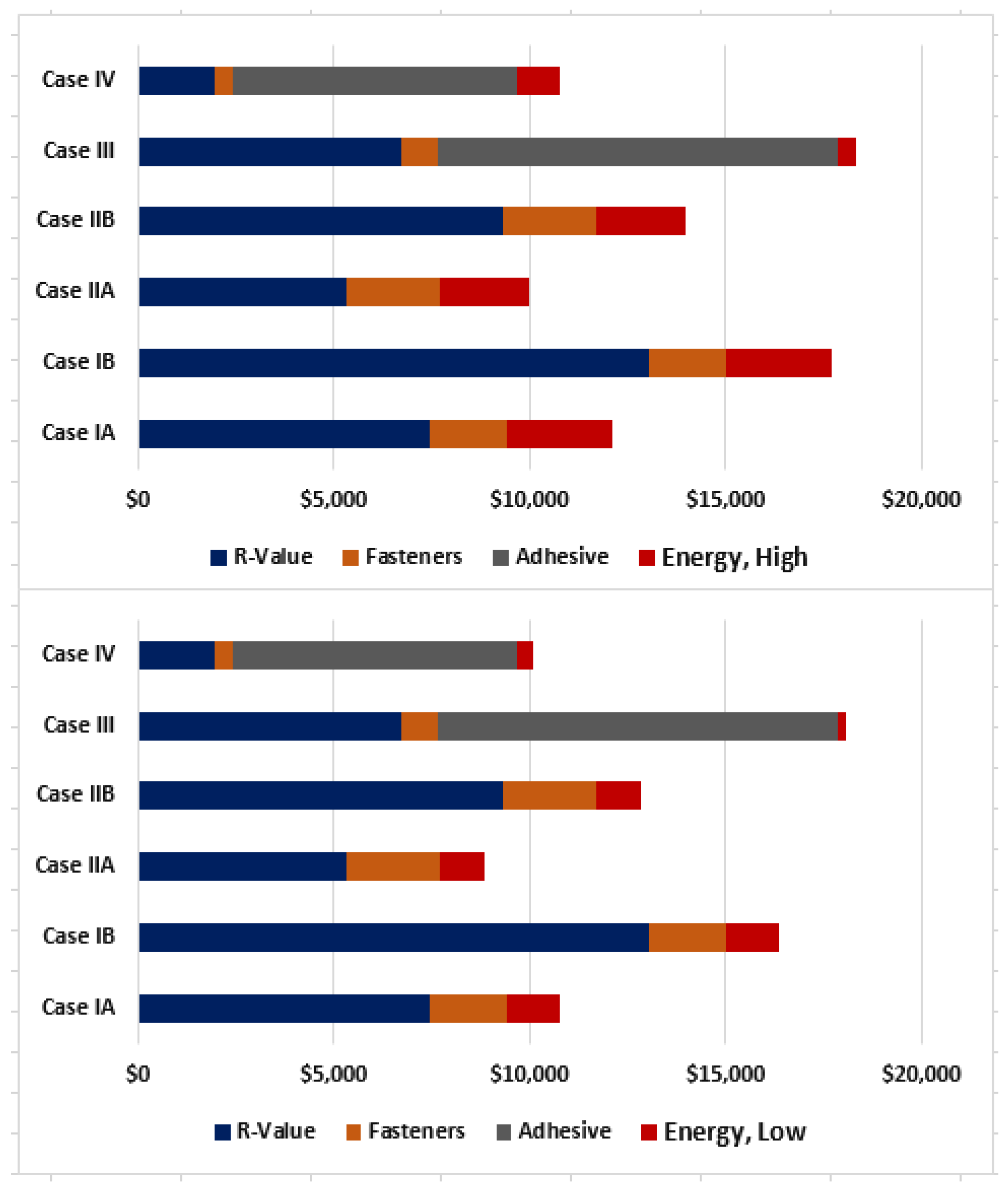
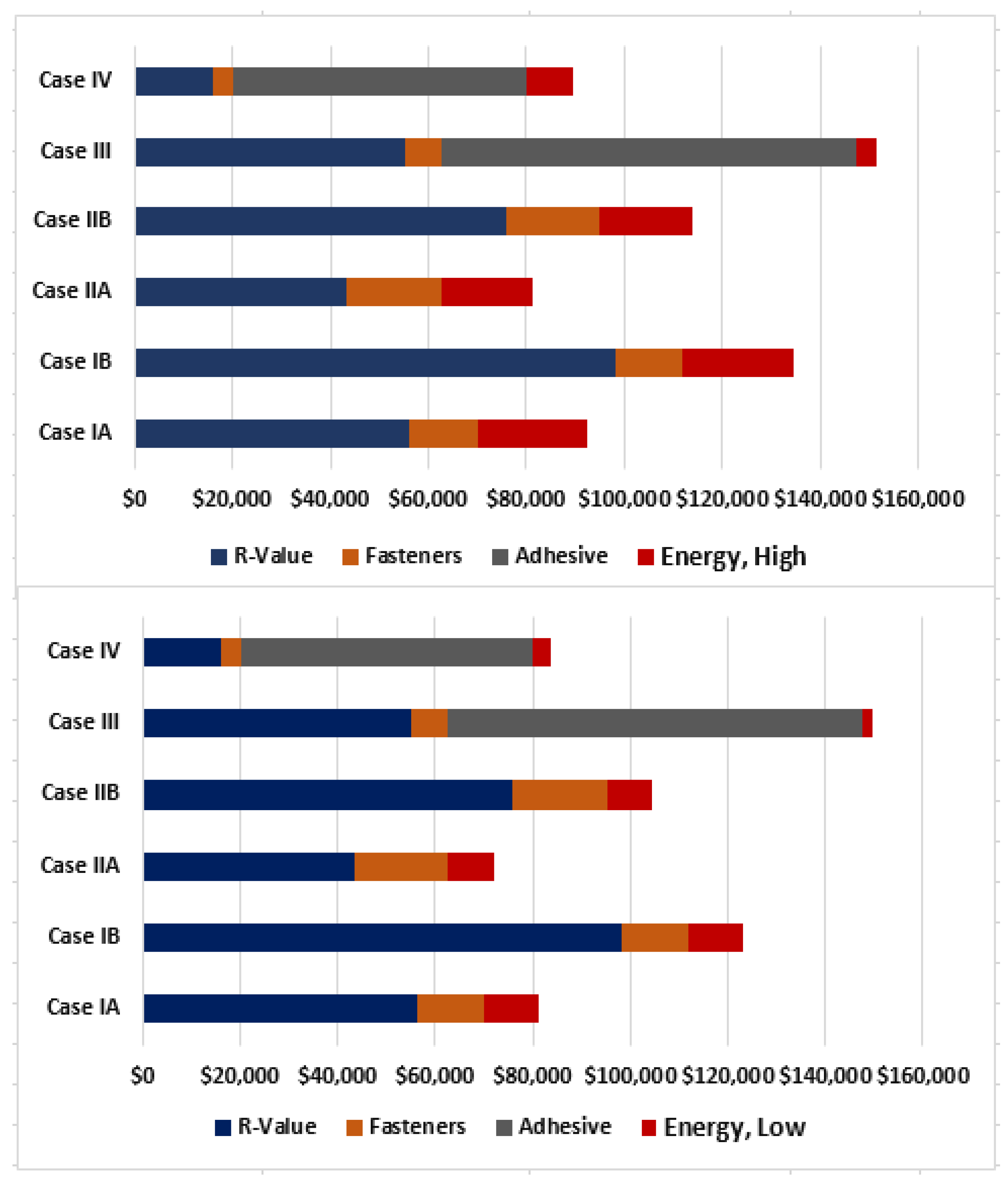
It was previously noted by Taylor and Hartwig that energy-efficiency costs do not correlate with location and climate but are dependent on local energy costs (for both heating and cooling) and, specifically, electricity demand charges [22]. Therefore, the highest and lowest costs of lost energy efficiency were used to compare the total overall costs, as shown in Figure 7, Figure 8 and Figure 9 for the three building sizes.
In the analysis for a 15,000 sq. ft. (1394 m2) building, Figure 9, the fully adhered system described by Case IV has the lowest total cost compared to the mechanically attached system, Case IA. For the 50,000 sq. ft. (4645 m2) building, Case IA and IV are essentially equivalent, while for the 125,000 sq. ft. (11,613 m2) building the mechanically attached system, Case IA, has a slightly lower overall cost versus the fully adhered Case IV.
7. Discussion
As described earlier, energy and building codes assume that roof insulation is continuous and that, therefore, the thermal insulation value intended by the architect or building designer is achieved. However, as indicated by prior work, the use of metal fasteners to attach insulation causes significant loss of insulation thermal value. Furthermore, single-ply roofing uses mechanical fastening as a cost-effective attachment method. To achieve required wind uplift resistance demands that fastener densities are quite high. This work has evaluated the thermal insulation losses caused by metal fasteners and found the losses to be high. In fact, the economic costs of lost insulation value are significant. As shown here by modeling, a mechanically attached roof system with two layers of polyiso insulation loses a little over 56,000 USD in purchased material in the case of the 125,000 sq. ft. (11,613 m2) roof. This type of system represents about 80% of the market (GAF Internal Sales Data for 2017). The cost of lost insulation value is increased in each system that uses high-density polyiso, i.e., Cases IB, IIB, and III, as would be expected due to the higher cost of such a product.
The system having the lowest loss in R-value or RSI is Case III, which uses a first layer of mechanically fastened high-density polyiso board. This achieves a system insulation level around 98.5% of the design insulation value. However, that system has a high economic cost due to the use of adhesives combined with the high-density polyiso insulation board.
Interestingly, the lowest total economic cost system is represented by Case IIA. This uses two layers of polyiso insulation and inductively heated plates for attachment. The overall fastener densities for this system are lower than for conventional screws and plates. This system could be improved upon by lowering the thickness of the bottom insulation board so long as wind uplift and other design requirements are met.
Once the loss of energy efficiency is factored in, then the fully adhered system is of similar or slightly lower total economic cost than the mechanically attached system, depending on building size. This would suggest that the mechanically attached assembly is only cost effective from an initial installation perspective. Once the loss of energy efficiency over a 15-year time frame is factored in, then these two systems are similar.
Taken overall, a number of points can be made if the goal is to improve the energy efficiency of buildings while factoring in the economic cost of doing so:
- Systems that are solely mechanically attached carry a high hidden economic cost due to the loss in insulation caused by thermal shortcircuiting. In other words, the insulation level specified by the architect is not actually achieved due to the high fastener levels used. The insulation level that was paid for is not actually achieved and, furthermore, this has long-term energy-efficiency costs for the building owner.
- When the 15-year cost of lost energy efficiency is added to the system costs associated with effective versus designed insulation levels, then a fully adhered system can be cost effective depending on building size. This argues that the initial cost savings achieved by using mechanical attachments are negated by the longer-term cost of reduced building energy efficiency.
- Case IV, a lower layer of mechanically attached polyiso insulation with all subsequent layers being fully adhered, had the lowest overall total cost once material and long-term energy-efficiency costs were calculated, and is worthy of further analysis. The loss in insulation level is the lowest and could potentially be reduced further if the lower layer could also be fully adhered. This might be achievable if a self-adhered vapor retarder were used at the deck level, for example.
- Fully adhered systems do not flutter or billow during high wind events, thereby eliminating the ingress of interior conditioned air up into the roof assembly. This latter phenomenon would naturally further reduce energy efficiency (see Molleti et al. [23] for example). Also, fully adhered systems such as described by Case IV have higher wind uplift strengths.
- With such significant deviations from design insulation value, there could be unintended impacts on dew-point calculations for mechanically attached assemblies. It should be noted that the modeled R-values used represent system averages. In practice, fasteners cause localized and far more dramatic shifts in dew point (e.g., corners) which would be out of the scope of this type of analysis to consider. However, by “burying” fasteners within a system, such as Case IV, any risks of condensation will be reduced.
It should be noted that the analysis shown here was based on material costs and did not take into account the cost of installation. Labor rates vary significantly by location and would need to be taken into account during any validation work.
Author Contributions
T.J.T. conceived of the project and contributed to the modeling and analysis; J.W. and J.R.K. contributed to the modeling and analysis, and reviewed the work; C.A.H. provided information about roof-system design and material costs, and reviewed the work.
Conflicts of Interest
The authors declare no conflict of interest.
References
- Synnefa, A.; Santamouris, M.; Apostolakis, K. On the Development, Optical Properties, and Thermal Performance of Cool Colored Paints for the Urban Environment. Sol. Energy 2007, 81, 488–497. [Google Scholar] [CrossRef]
- Levinson, R.; Akbari, H. Potential Benefits of Cool Roofs on Commercial Buildings: Conserving Energy, Saving Money, and Reducing Emission of Greenhouse Gases and Air Pollutants. Energy Eff. 2010, 3, 53–109. [Google Scholar] [CrossRef]
- Costanzo, V.; Evola, G.; Marletta, L. Cool Roofs for Passive Cooling: Performance in Different Climates and for Different Insulation Levels in Italy. Adv. Build. Energy Res. 2013, 7, 155–169. [Google Scholar] [CrossRef]
- International Code Council. International Energy Conservation Code; ICC: Washington, DC, USA, 2015. [Google Scholar]
- American Society of Heating, Refrigerating, and Air Conditioning Engineers. ANSI/ASHRAE/IES Standard 90.1-2013, Energy Standards for Buildings Except Low-Rise Residential Buildings; ASHRA: Atlanta, GA, USA, 2013. [Google Scholar]
- Burch, D.M.; Shoback, P.J.; Cavanaugh, K. A Heat Transfer Analysis of Metal Fasteners in Low-Slope Roofs. In Roofing Research and Standards Development; ASTM International: West Conshohocken, PA, USA, 1987; pp. 10–22. [Google Scholar]
- Olson, E.K.; Saldanha, C.M.; Hsu, J.W. Thermal Performance Evaluation of Roofing Details to Improve Thermal Efficiency and Condensation Resistance. In Roofing Research and Standards Development; STP1590; Molleti, S., Rossiter, W.J., Eds.; ASTM International: West Conshohocken, PA, USA, 2015; Volume 8, pp. 10–22. [Google Scholar]
- Singh, M.; Gulati, R.; Srinivasan, R.S.; Bhandari, M. Three-Dimensional Heat Transfer Analysis of Metal Fasteners in Roofing Assemblies. Buildings 2016, 6, 49. [Google Scholar] [CrossRef]
- Pallin, P.; Kehrer, M.; Desjarlais, A. The Energy Penalty Associated With the Use of Mechanically Attached Roofing Systems. In Proceedings of the Symposium on Building Envelope Technology, Tampa, FL, USA, 20–21 October 2014. [Google Scholar]
- Cool Roof Rating Council. Available online: http://coolroofs.org/products/results (accessed on 11 October 2017).
- Petrie, T.W.; Atchley, J.A.; Childs, P.W.; Desjarlais, A.O. Effect of Solar Radiation Control on Energy Costs—A Radiation Control Fact Sheet for Low-Slope Roofs. In Performance of the Exterior Envelopes of Whole Buildings VIII: Integration of Building Envelopes; ASHRAE: Atlanta, GA, USA, 2001. [Google Scholar]
- Petrie, T.W.; Wilkes, K.E.; Desjarlais, A.O. Effect of Solar Radiation Control on Energy Costs—An Addition to the DOE Cool Roof Calculator. In Performance of Exterior Envelopes of Whole Buildings IX; ASHRAE: Atlanta, GA, USA, 2004. [Google Scholar]
- Ornl Roof Savings Calculator. Available online: http://rsc.ornl.gov/ (accessed on 11 October 2017).
- ORNL Cool Roof Calculator with Peak Demand. Available online: http://web.ornl.gov/sci/buildings/tools/cool-roof/peak/ (accessed on 11 October 2017).
- US Department of Energy, Office of Energy Efficiency and Renewable Energy. Buildings Energy Data Book; EERE: Washington, DC, USA, 2011.
- Energy Information Agency. Available online: https://www.eia.gov/dnav/ng/ng_pri_sum_dcu_nus_a.htm (accessed on 11 October 2017).
- Energy Information Agency. Table 5.6B. Available online: https://www.eia.gov/electricity/monthly/archive/february2017.pdf (accessed on 11 October 2017).
- OpEI Utility Rate Database. Available online: https://openei.org/wiki/Utility_Rate_Database (accessed on 11 October 2017).
- US Energy Information Administration. Annual Energy Outlook 2017. Available online: https://www.eia.gov/outlooks/aeo/pdf/0383(2017).pdf (accessed on 5 January 2017).
- Polyiso Manufacturers Association. Available online: http://www.polyiso.org/?page=LTTRQM (accessed on 6 November 2017).
- Cusick, M.; Wang, L.; Griffin, C. New LTTR Values and What They Mean for Roofing Industry Professionals; Roofing Contractor: Troy, MI, USA, 2014. [Google Scholar]
- Taylor, T.J.; Hartwig, C. Cool Roof Use in Commercial Buildings in the United States: An Energy Cost Analysis. In Proceedings of the ASHRAE Winter Conference, (ASHRAE, CH-18-009), Chicago, IL, USA, 20–24 January 2018. [Google Scholar]
- Molleti, S.; Baskaran, B.; Kalinger, P.; Graham, M.; Cote, J.F.; Malpezzi, J.; Schwetz, J. Evaluation of Air Leakage Properties of Seam-Fastened Mechanically Attached Single-Ply and Polymer-Modified Bitumen Roof Membrane Assemblies. In Roofing Research and Standards Development; STP1590; Molleti, S., Rossiter, W.J., Eds.; ASTM International: West Conshohocken, PA, USA, 2015; Volume 8, pp. 30–43. [Google Scholar]
Figure 1.
A big box, rectangular roof showing the three zones—field, perimeter, and corner.
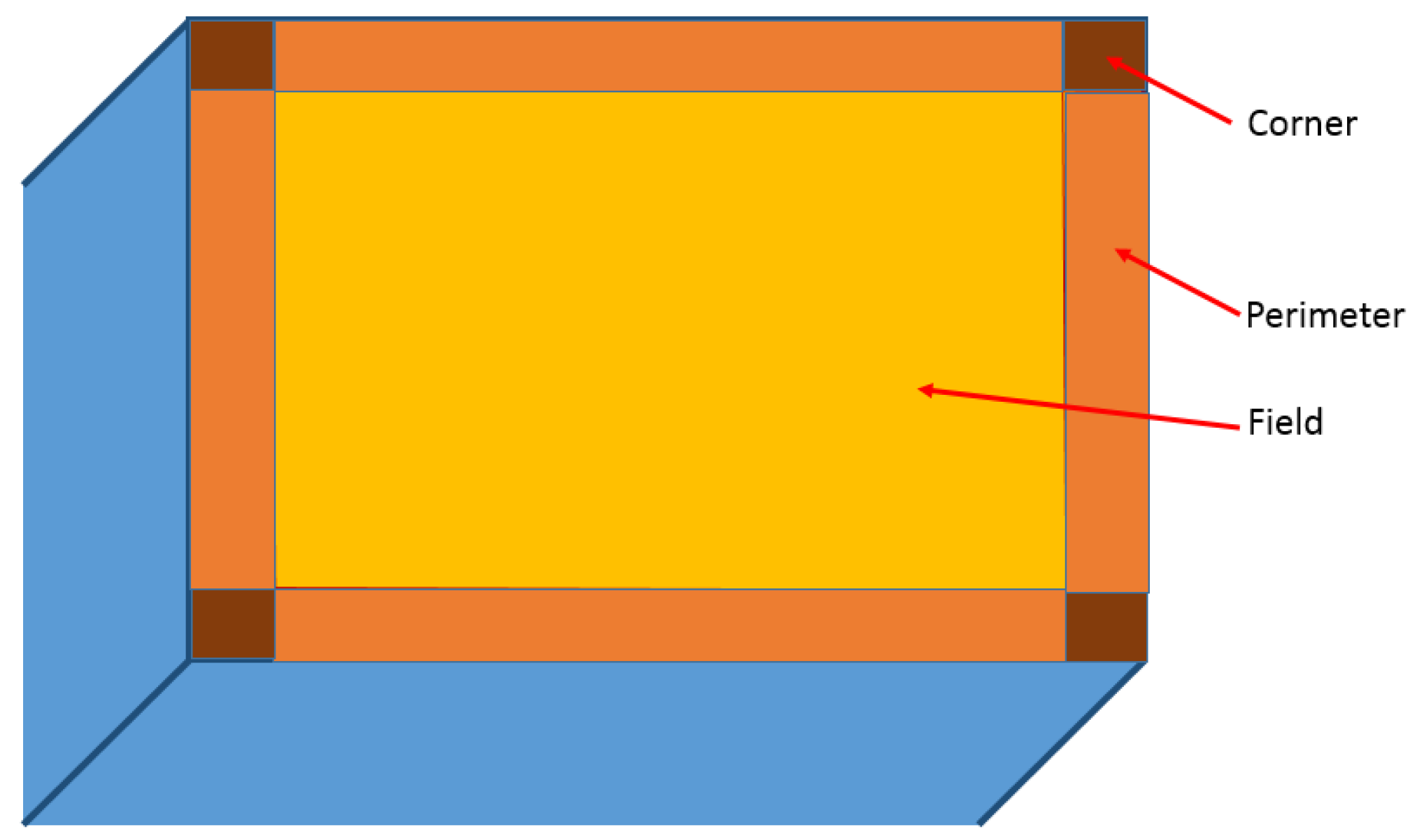
Figure 2.
Schematic showing single-ply membrane layout and mechanical fastening.

Figure 3.
Analysis of the effects of insulation fastener configuration on insulation value results shown by Olson et al. [10] to show percent reduction from design R-value (y) as a function of overall roof fastener density (x), where the straight line fit is expressed as y = 23.851x + 5.0192.
Figure 3.
Analysis of the effects of insulation fastener configuration on insulation value results shown by Olson et al. [10] to show percent reduction from design R-value (y) as a function of overall roof fastener density (x), where the straight line fit is expressed as y = 23.851x + 5.0192.
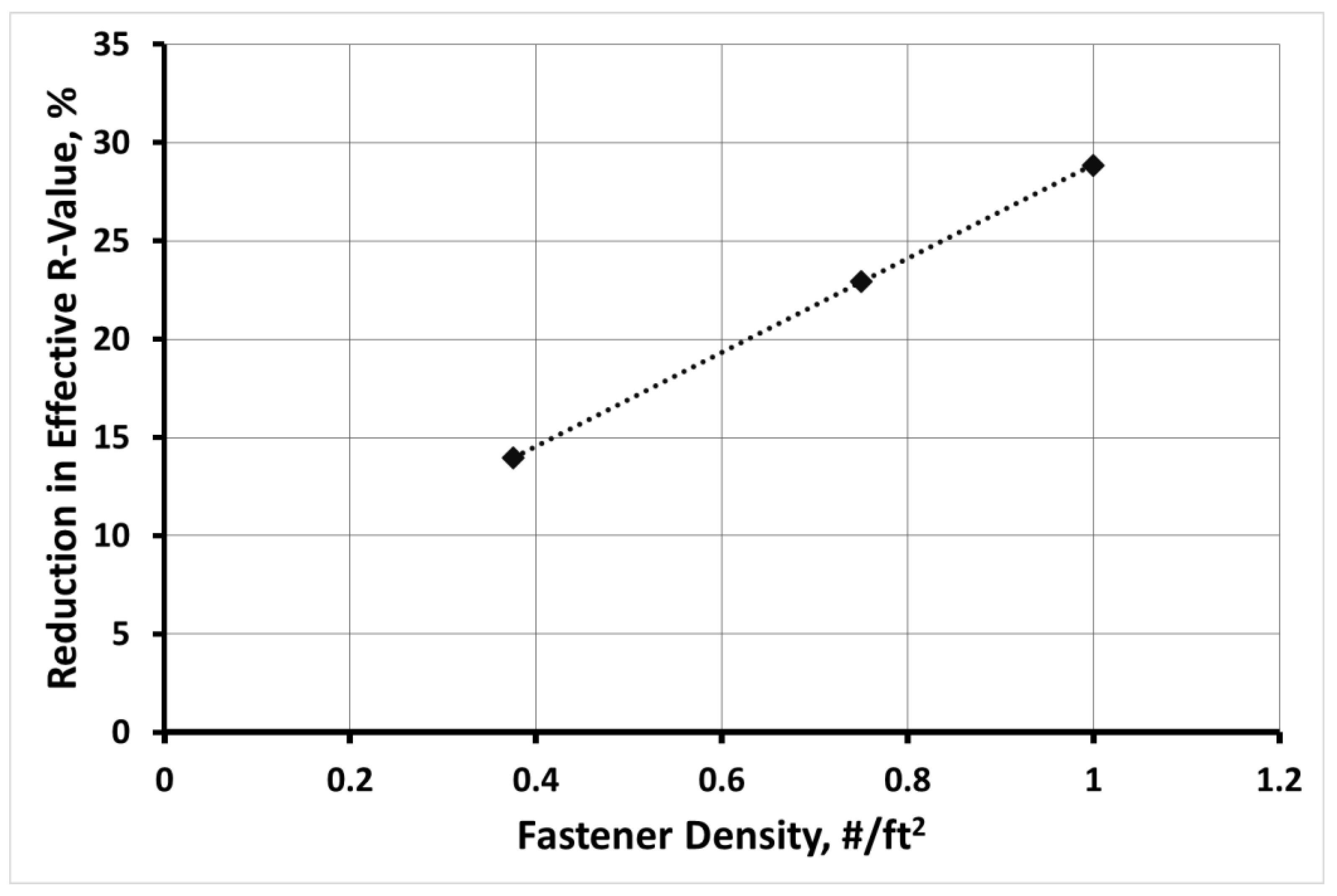
Figure 4.
The costs associated with deviating from a design R 30, due to lost R-value and fastener and adhesive costs for a 125,000 square foot (11,613 m2) building.
Figure 4.
The costs associated with deviating from a design R 30, due to lost R-value and fastener and adhesive costs for a 125,000 square foot (11,613 m2) building.
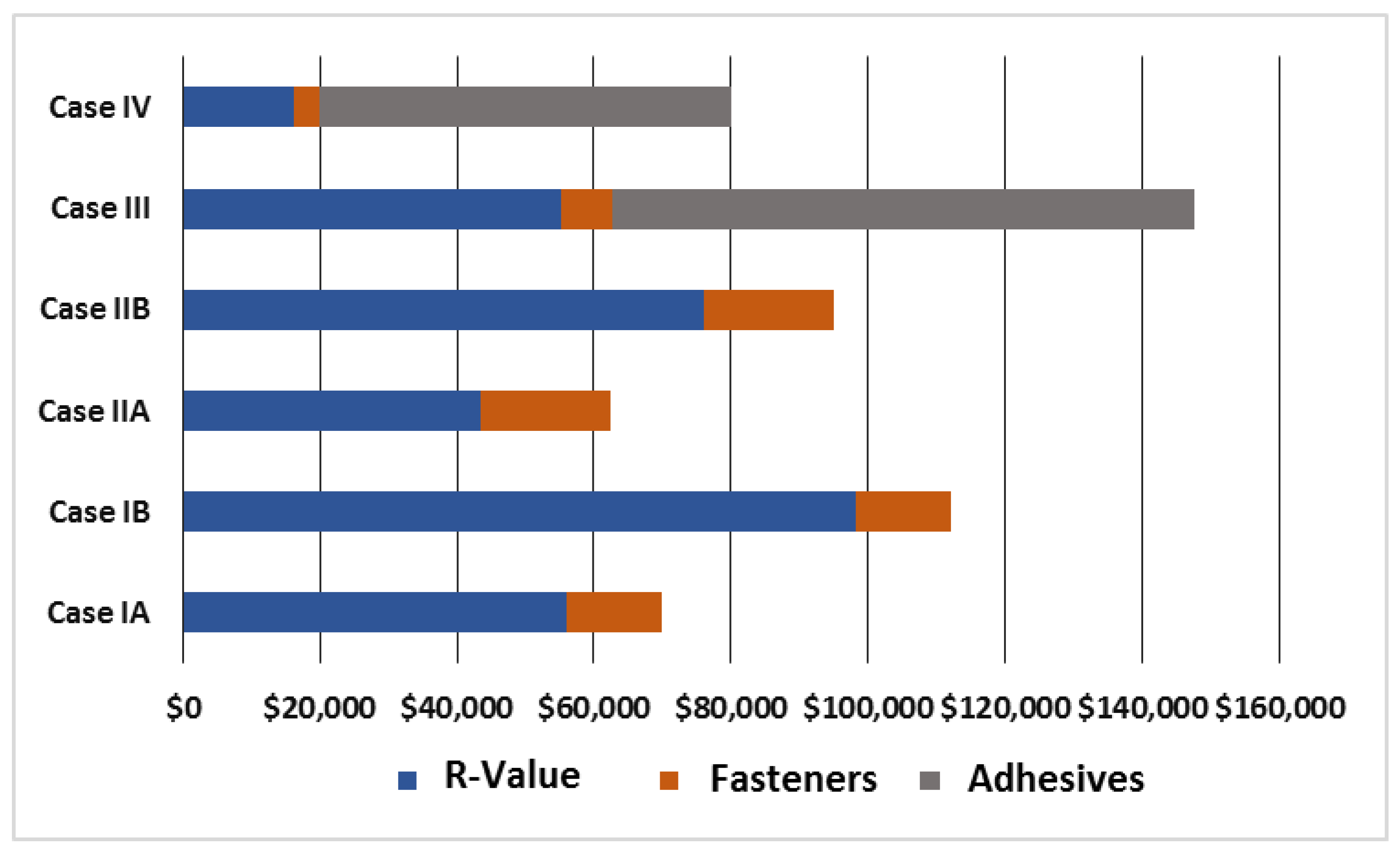
Figure 5.
The costs associated with deviating from a design R 30, due to lost R-value and fastener and adhesive costs for a 50,000 square foot 11,613 m2) building.
Figure 5.
The costs associated with deviating from a design R 30, due to lost R-value and fastener and adhesive costs for a 50,000 square foot 11,613 m2) building.
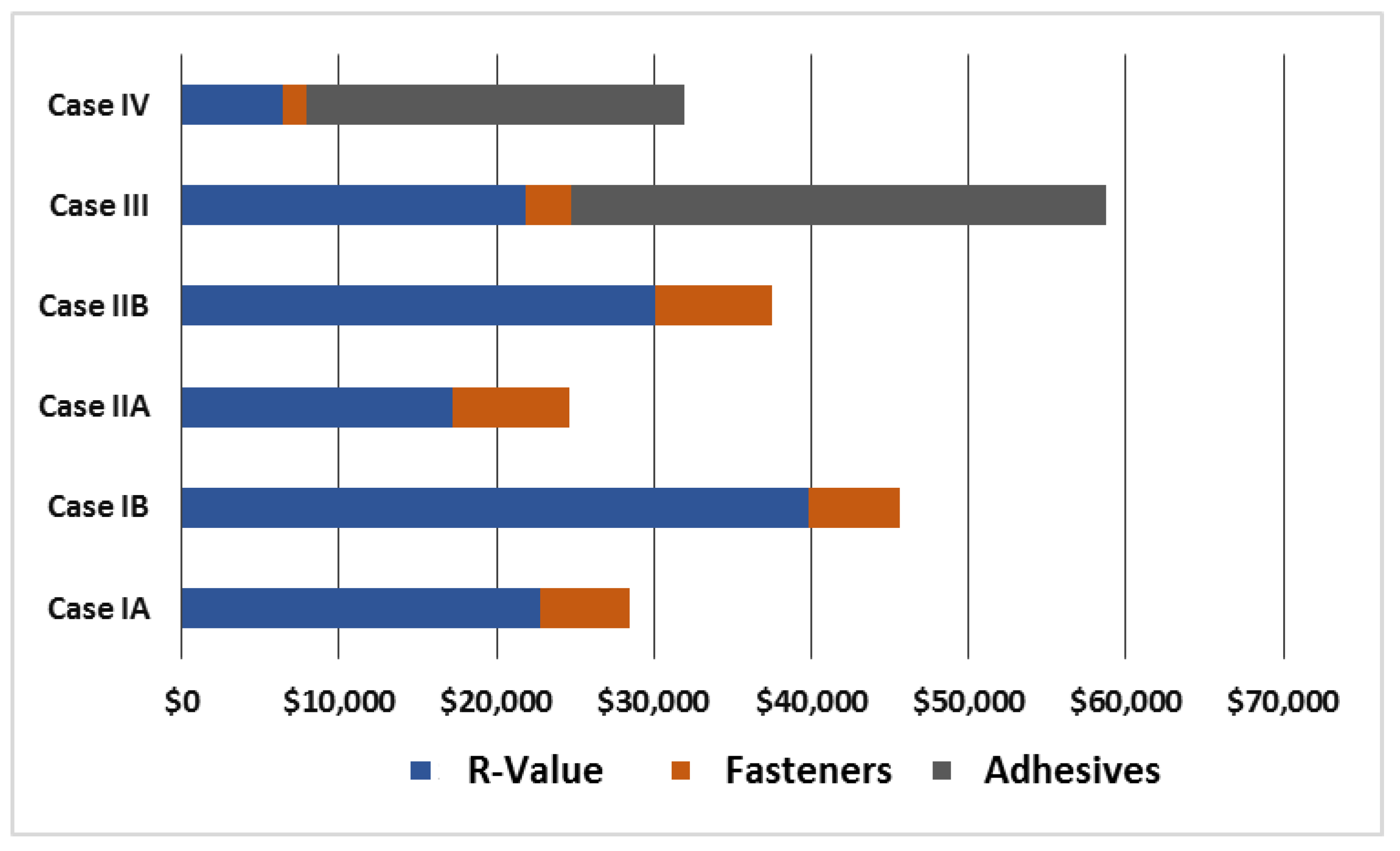
Figure 6.
The costs associated with deviating from a design R 30, due to lost R-value and fastener and adhesive costs for a 15,000 square foot (1394 m2) building.
Figure 6.
The costs associated with deviating from a design R 30, due to lost R-value and fastener and adhesive costs for a 15,000 square foot (1394 m2) building.

Figure 7.
The costs associated with deviating from a R 30 (RSI 5.283) design, due to lost R-value, fastener and adhesive costs, and lost energy efficiency for a 125,000 square foot (11,613 m2) building. The upper chart is for the largest potential cost of lost energy efficiency, and the lower chart is for the smallest potential cost of lost energy efficiency. All costs are in USD.

Figure 8.
The costs associated with deviating from a R 30 (rsi 5.283) design, due to lost R-value, fastener and adhesive costs, and lost energy efficiency for a 50,000 square foot (4645 m2) building. The upper chart is for the largest potential cost of lost energy efficiency, and the lower chart is for the smallest potential cost of lost energy efficiency. All costs are in USD.
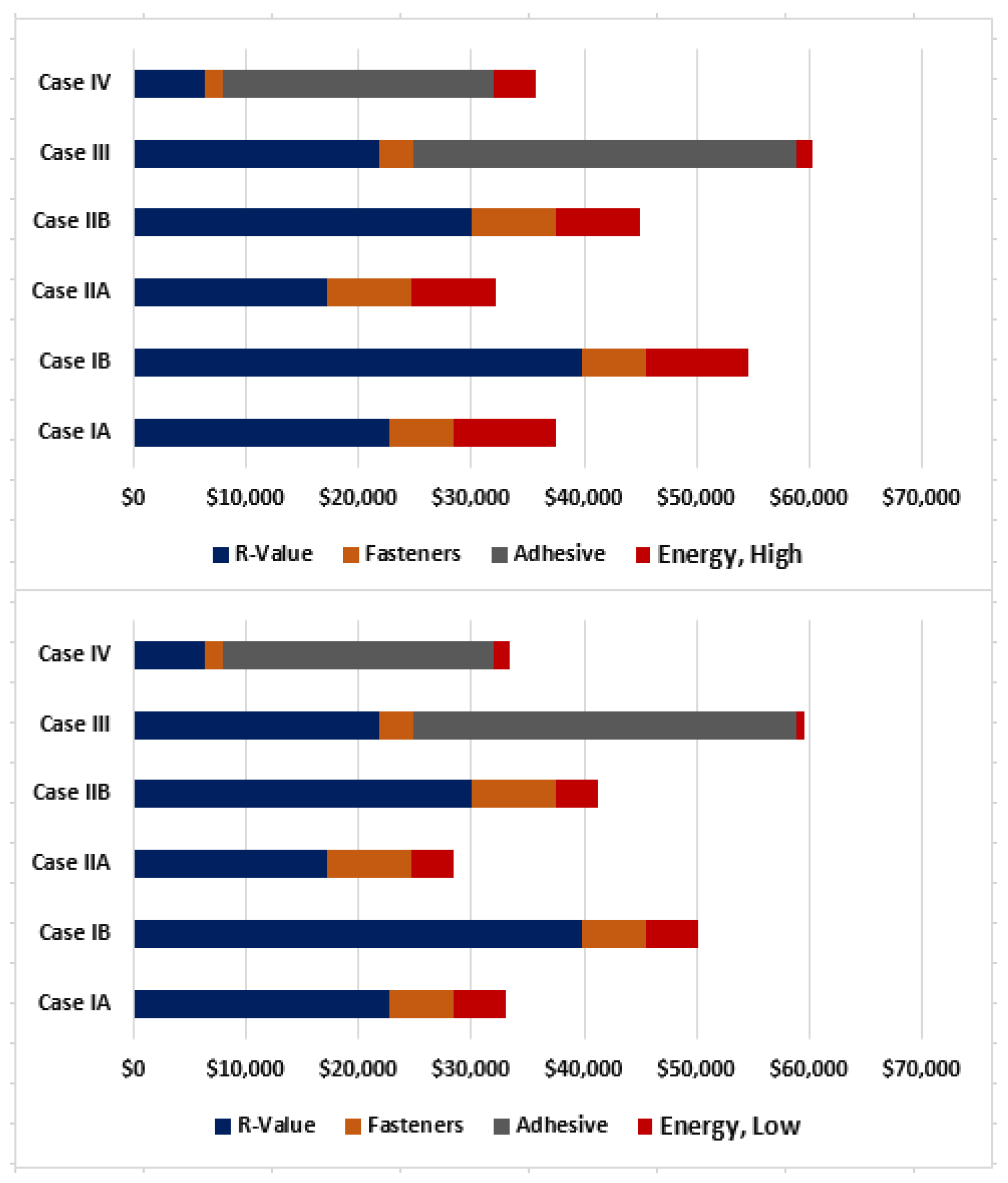
Figure 9.
The costs associated with deviating from a R 30 (RSI 5.283) design, due to lost R-value, fastener and adhesive costs, and lost energy efficiency for a 15,000 square foot (1394 m2) building. The upper chart is for the largest potential cost of lost energy efficiency, and the lower chart is for the smallest potential cost of lost energy efficiency. All costs are in USD.

Table 1.
The percent loss in effective insulation value in different roof zones, as modeled by Olson et al. [7].
Table 1.
The percent loss in effective insulation value in different roof zones, as modeled by Olson et al. [7].
| Roof Zone | Fastener Density Per 100 ft2 (per m2) | % Loss from Designed R-Value | |
|---|---|---|---|
| Gypsum Cover Board | Polyiso Cover Board | ||
| Field | 37.5 (4.04) | 13.95 | 12.82 |
| Perimeter | 75.0 (8.08) | 22.94 | 22.72 |
| Corner | 100 (10.78) | 28.85 | 27.64 |
Table 2.
Description of roofing assembles analyzed in this study, with above-steel-deck components listed.
Table 2.
Description of roofing assembles analyzed in this study, with above-steel-deck components listed.
| Case IA |  |
| Insulation—R 30 (RSI 5.283) total, installed as two layers, 3 in. (7.62 cm) R 17.4 (RSI 3.064) and 2.2 in. (5.59 cm) R 12.6 (RSI 2.219). Mechanically attached. Membrane—mechanically attached. | |
| Case IB |  |
| Insulation—R-30 (RSI 5.283) total, installed as three layers, ½ in. (1.27 cm) R 2.5 (RSI 0.440), 2.5 in. (6.35 cm) R 14.4 (RSI 2.536), and 2.3 in. (5.84 cm) R 13.1 (RSI 2.307), mechanically attached. Membrane—mechanically attached. | |
| Case IIA |  |
| Insulation—R 30 (RSI 5.283) total, installed as two layers, 3 in. (7.62 cm) R 17.4 (RSI 3.064) and 2.2 in. (5.59 cm) R 12.6 (RSI 2.219). Mechanically attached using induction welding plates. Membrane—attached via induction welding to insulation plates. | |
| Case IIB |  |
| Insulation—R-30 (RSI 5.283) total, installed as three layers, ½ in. (1.27 cm) R 2.5 (RSI 0.440), 2.3 in. (5.84 cm) R 13.1 (RSI 2.307), and 2.5 in. (6.35 cm) R 14.4 (RSI 2.536). Mechanically attached using induction welding plates. Membrane—attached via induction welding to insulation plates. | |
| Case III |  |
| Insulation—R 30 (RSI 5.283) total, installed as three layers, ½ in. (1.27 cm) R 2.5 (RSI 0.440), mechanically attached, 2.3 in. (5.84 cm) R 13.1 (RSI 2.307) and 2.5 in. (6.35 cm) R 14.4 (RSI 2.536), each adhered. Membrane—fully adhered. | |
| Case IV |  |
| Insulation—R 30 (RSI 5.283) total, 2.0 in. (3.81 cm) R 11.4 (RSI 2.008) mechanically attached, 3.7 in. (8.64 cm) R 19.1 (RSI 3.364), and ½ in. (1.27 cm) R 2.5 (RSI 0.440) each adhered. Membrane—fully adhered. |
Table 3.
Insulation fastener densities (e.g., use rates), per 4 × 8 ft. (122 × 244 cm) polyiso board.
Table 3.
Insulation fastener densities (e.g., use rates), per 4 × 8 ft. (122 × 244 cm) polyiso board.
| Assembly | Roof Zone, Fastener per 4 × 8 ft. Polyiso Board | Roof Zone, Fastener per m2 Polyiso Board | ||||
|---|---|---|---|---|---|---|
| Field | Perimeter | Corner | Field | Perimeter | Corner | |
| Case IA | 5 | 5 | 5 | 1.68 | 1.68 | 1.68 |
| Case IB | ||||||
| Case IIA | 8 | 15 | 20 | 2.69 | 5.04 | 6.72 |
| Case IIB | ||||||
| Case III | 16 | 24 | 32 | 5.37 | 8.06 | 10.75 |
| Case IV | 8 | 12 | 16 | 2.69 | 4.03 | 5.37 |
Table 4.
Overall fastener densities, calculated as number of fasteners per square foot of roof area.
Table 4.
Overall fastener densities, calculated as number of fasteners per square foot of roof area.
| Fastener Density, per ft2 | Fastener Density, per m2 | |||||
|---|---|---|---|---|---|---|
| Building Area | 125,000 ft2 | 50,000 ft2 | 15,000 ft2 | 11,613 m2 | 4645 m2 | 1394 m2 |
| Case IA | 0.4166 | 0.4266 | 0.4843 | 0.0387 | 0.0396 | 0.0450 |
| Case IB | ||||||
| Case IIA | 0.2751 | 0.2693 | 0.2860 | 0.0256 | 0.0250 | 0.0266 |
| Case IIB | ||||||
| Case III | 0.5289 | 0.5221 | 0.5417 | 0.0491 | 0.0485 | 0.0503 |
| Case IV | 0.2644 | 0.2611 | 0.2708 | 0.0246 | 0.0243 | 0.0252 |
Table 5.
Energy-cost data for commercial customers, averaged for 2016.
| City, State | Climate Zone | Electric Cost, USD/kWhr | Demand Charge, USD/kW | Gas Cost, USD/1000 cu ft. | Gas Cost, USD/Therm | Gas Cost, USD/100 cu meter |
|---|---|---|---|---|---|---|
| Miami, FL | 1 | 0.0911 | 9.2 | 10.42 | 1.042 | 36.80 |
| Houston, TX | 2 | 0.0771 | 5.477 | 6.89 | 0.689 | 24.33 |
| Fresno, CA | 3 | 0.1515 | 13.32 | 8.42 | 0.842 | 29.73 |
| Nashville, TN | 4 | 0.1003 | 9.67 | 7.8 | 0.78 | 27.55 |
| Albany, NY | 5 | 0.1447 | 10.27 | 6.18 | 0.618 | 21.82 |
| Minneapolis, MN | 6 | 0.0988 | 12.32 | 6.44 | 0.644 | 22.74 |
Table 6.
Effective R-values for each of the modeled assemblies, all based on an R 30 (RSI 5.283) design.
Table 6.
Effective R-values for each of the modeled assemblies, all based on an R 30 (RSI 5.283) design.
| Effective Insulation Value, R-Value | Effective Insulation Value, RSI | |||||
|---|---|---|---|---|---|---|
| Building Size | 125,000 ft2 | 50,000 ft2 | 15,000 ft2 | 11,613 m2 | 4645 m2 | 1394 m2 |
| Case IA | 25.514 | 25.442 | 25.029 | 4.493 | 4.481 | 4.408 |
| Case IB | ||||||
| Case IIA | 26.526 | 26.568 | 26.447 | 4.672 | 4.679 | 4.658 |
| Case IIB | ||||||
| Case III | 29.559 | 29.563 | 29.552 | 5.206 | 5.206 | 5.204 |
| Case IV | 28.709 | 28.718 | 28.691 | 5.056 | 5.058 | 5.053 |
Table 7.
Effective R-value shown as a percentage of the R-30 (RSI 5.283) design. (This was calculated using the effective insulation values shown in Table 6).
Table 7.
Effective R-value shown as a percentage of the R-30 (RSI 5.283) design. (This was calculated using the effective insulation values shown in Table 6).
| Reduction in Insulation Value | |||
|---|---|---|---|
| Building Size | 125,000 ft2 (11,613 m2) | 50,000 ft2 (4645 m2) | 15,000 ft2 (1394 m2) |
| Case IA | 85.05% | 84.81% | 83.43% |
| Case IB | |||
| Case IIA | 88.42% | 88.56% | 88.16% |
| Case IIB | |||
| Case III | 98.53% | 98.54% | 98.51% |
| Case IV | 95.70% | 95.73% | 95.64% |
Table 8.
Economic cost of reduction from design to effective insulation value for each assembly, in terms of the cost of an equivalent thickness of polyiso.
Table 8.
Economic cost of reduction from design to effective insulation value for each assembly, in terms of the cost of an equivalent thickness of polyiso.
| Cost of Lost Insulation Value, USD | |||
|---|---|---|---|
| Building Size | 125,000 ft2 (11,613 m2) | 50,000 ft2 (4645 m2) | 15,000 ft2 (1394 m2) |
| Case IA | 56,079 | 22,792 | 7456 |
| Case IB | 98,138 | 39,885 | 13,048 |
| Case IIA | 43,424 | 17,162 | 5329 |
| Case IIB | 75,991 | 30,033 | 9325 |
| Case III | 55,103 | 21,841 | 6727 |
| Case IV | 16,140 | 6410 | 1963 |
Table 9.
Total fastener costs for each roofing system.
| Cost of Fasteners, USD | |||
|---|---|---|---|
| Building Size | 125,000 ft2 (11,613 m2) | 50,000 ft2 (4645 m2) | 15,000 ft2 (1394 m2) |
| Case IA | 13,892 | 5691 | 1938 |
| Case IB | |||
| Case IIA | 19,099 | 7478 | 2384 |
| Case IIB | |||
| Case III | 7470 | 2950 | 918 |
| Case IV | 3900 | 1540 | 479 |
Table 10.
Adhesive costs for each roofing assembly.
| Cost of Adhesive, USD | |||
|---|---|---|---|
| Building Size | 125,000 ft2 (11,613 m2) | 50,000 ft2 (4645 m2) | 15,000 ft2 (1394 m2) |
| Case IA | $0 | $0 | $0 |
| Case IB | |||
| Case IIA | $0 | $0 | $0 |
| Case IIB | |||
| Case III | $85,000 | $34,000 | $10,200 |
| Case IV | $60,000 | $24,000 | $7,200 |
Table 11.
Total 15-year cost of lost energy Eefficiency due to the effective R-values compared to the design R-30, all values being USD. Three-year aged membrane reflectance and emissivity values were assumed.
Table 11.
Total 15-year cost of lost energy Eefficiency due to the effective R-values compared to the design R-30, all values being USD. Three-year aged membrane reflectance and emissivity values were assumed.
| Assembly | Case IA & IB | Case IIA & IIB | Case III | Case IV | ||||||||
|---|---|---|---|---|---|---|---|---|---|---|---|---|
| Building Size, s.f. | 125,000 | 50,000 | 15,000 | 125,000 | 50,000 | 15,000 | 125,000 | 50,000 | 15,000 | 125,000 | 50,000 | 15,000 |
| Building Size, m2 | 11,613 | 4645 | 1394 | 11,613 | 4645 | 1394 | 11,613 | 4645 | 1394 | 11,613 | 4645 | 1394 |
| Miami, FL | $18,750 | $7500 | $2250 | $15,000 | $6000 | $1800 | $3750 | $1500 | $450 | $7500 | $3750 | $1125 |
| Houston, TX | $11,250 | $4500 | $1350 | $9375 | $3750 | $1125 | $1875 | $750 | $225 | $5625 | $2250 | $675 |
| Fresno, CA | $22,500 | $9000 | $2700 | $18,750 | $7500 | $2250 | $3750 | $1500 | $450 | $9375 | $3750 | $1125 |
| Nashville, TN | $13,125 | $5250 | $1575 | $11,250 | $4500 | $1350 | $1875 | $750 | $225 | $5625 | $2250 | $675 |
| Albany, NY | $11,250 | $4500 | $1350 | $9375 | $3750 | $1125 | $1875 | $750 | $225 | $5625 | $2250 | $675 |
| Minneapolis, MN | $11,250 | $4500 | $1350 | $9375 | $3750 | $1125 | $1875 | $750 | $225 | $3750 | $1500 | $450 |
© 2018 by the authors. Licensee MDPI, Basel, Switzerland. This article is an open access article distributed under the terms and conditions of the Creative Commons Attribution (CC BY) license (http://creativecommons.org/licenses/by/4.0/).
Share and Cite
MDPI and ACS Style
Taylor, T.J.; Willits, J.; Hartwig, C.A.; Kirby, J.R. Optimizing Single-Ply Low-Slope Roofing Assemblies for Insulation Value. Buildings 2018, 8, 64. https://doi.org/10.3390/buildings8050064
AMA Style
Taylor TJ, Willits J, Hartwig CA, Kirby JR. Optimizing Single-Ply Low-Slope Roofing Assemblies for Insulation Value. Buildings. 2018; 8(5):64. https://doi.org/10.3390/buildings8050064
Chicago/Turabian StyleTaylor, Thomas J., James Willits, Christian A. Hartwig, and James R. Kirby. 2018. "Optimizing Single-Ply Low-Slope Roofing Assemblies for Insulation Value" Buildings 8, no. 5: 64. https://doi.org/10.3390/buildings8050064
Note that from the first issue of 2016, this journal uses article numbers instead of page numbers. See further details here.