Enhancing Heat Treatment Efficacy for Insect Pest Control: A Case Study of a CFD Application to Improve the Design and Structure of a Flour Mill

Abstract

Heat treatment of the indoor environment of flour mills is an alternative technique to chemical fumigation for controlling insect pests. The aim of this research was to assess temperature distribution inside a flour mill during a heat treatment for insect pest control by computational fluid dynamics (CFD) modelling and simulation. The model was validated by using the average values of experimental data acquired during a heat treatment carried out in a flour mill, which is representative of the building materials and techniques used in the milling industry of South Italy. Simulations were carried out in steady-state conditions, and simulated data were validated by the average values of air and wall temperature measurements. Since the modelled temperature distribution in the mill fit the real one with a good accuracy (maximum error equal to 2.57 °C), the CFD model was considered reliable to simulate other operating conditions. Since it was observed that the internal surface temperatures of the mill were much lower than the value required for the success of the heat treatment, equal to 45 °C, the CFD model could be used for improving the effectiveness of heat treatments in the flour mill. Application of the proposed CFD model in the simulation of specific interventions could be aimed at improving both building performance and fan heaters’ localisation, in order to find the best configuration.

1. Introduction

Milling is the operation of grinding cereals to produce semolina or flour, which are then used in the food industry for the production of bread, pasta, and other derivatives.

One of the most important concerns in the milling phase is the proliferation of rodents and insect pests at different life stages, from eggs and larva until the adult form, within the processing environment [1]. This is due to the huge amounts of products treated in the mill that represents the ideal habitat for the proliferation of these pests, with negative consequences on hygiene and quality of the final products.

Pest control can be achieved by using different approaches, ranging from the use of chemical protectants, such as gaseous fumigants, to physical treatments [2].

Chemical fumigations with methyl bromide combined with other kinds of approved aerosol insecticides were widely used in the recent past because of the efficient level of disinfestation. However, in 1987, after the Montreal Protocol prohibited the use of substances considered harmful for the ozone layer, methyl bromide was phased out and banned permanently by 2005 [3]. In addition, another condition that has manifested during the recent years and pushed towards the abandonment of chemical methods for pest control regarded the increased resistance of pests to insecticides and gaseous fumigants [4].

During the years, many techniques alternative to the use of methyl bromide have been investigated. These studies lead to the development of integrated pest management (IPM) strategies, ecologically valid as based on both farming methods suitable to cultivation and continuous crop monitoring to control pests and reduce pesticide use [5]. Among IPM strategies, the heat treatment of the processing environment does not require the use of toxic substances, yet exposes the parasites to high temperatures, causing their death by dehydration or alteration of the basic organism functions [3]. The lethal effect of the treatment depends on both temperature levels and exposure time [6,7,8,9,10]. Even if the treatment was not lethal for the pests, it would have an adverse effect on their reproduction.

The heat treatment causes unusual temperatures and air movements within the production environment of the mill. The temperature increase in the building depends on a number of parameters related to the building, such as its location, the external climatic conditions, and the characteristics of the building components (e.g., the presence of an insulated building envelope). Noticeably, also, the equipment used for the heat treatment, as well as the related energy power, strongly affect the resulting indoor temperature field. Therefore, it is necessary to develop a model that, once validated, would allow selection of the most appropriate strategy for optimisation of the treatment and minimisation of energy costs, which economically affect its execution and sustainability. Therefore, the objective of this research study was the development of a specifically designed model by using a CFD (computational fluid dynamic) approach.

CFD modelling was introduced for the first time in the seventies by Nielsen for the study of the air movement within a ventilated room [11]. In the HVAC (heating, ventilating, and air conditioning) industry, CFD method has often been used for the analysis of wind pressure on building surfaces, and for the study of pollution of their indoor environments [12,13,14,15,16,17]. In flour mills, CFD has been applied to analyse leakage during fumigation [16,18,19].

To the authors’ knowledge, the use of a CFD model to study the thermal behaviour of a mill during the heat treatment for insect pest control has not been investigated, so far, in research works published in the literature. Therefore, in this study, an improvement of the state of the art was achieved by building a CFD model suitable for simulating the thermal behaviour of a mill floor when forced ventilation is produced in the indoor environment by the fan heaters that are usually utilised to raise the air temperature up to levels lethal to insects.

Firstly, the building components of the mill as well as the equipment used for the grain processing were geometrically surveyed and modelled by computer aided design (CAD) software. Moreover, the position of the electric fan heaters, as well as their technical specifications, i.e., ventilation rate and outlet air temperature, were acquired from the company that carried out the heat treatment, and they were included in the model. Indoor air temperatures were monitored before, during, and after the heat treatment at different time intervals, and in several locations of the building indoor environment, by using data-loggers equipped with air temperature probes. Surface temperatures of the thermal bridges of the mill, which are the most critical building components during the heat treatment, were mapped by using a thermal camera during the heat treatment, within a time interval characterised by a steady-state condition of the indoor air temperature.

After CFD model building, CFD model validation was performed to prove the accuracy and reliability of CFD simulations [20], and avoid uncertainties in the computer results [21].

2. Materials and Methods

2.1. Case Study

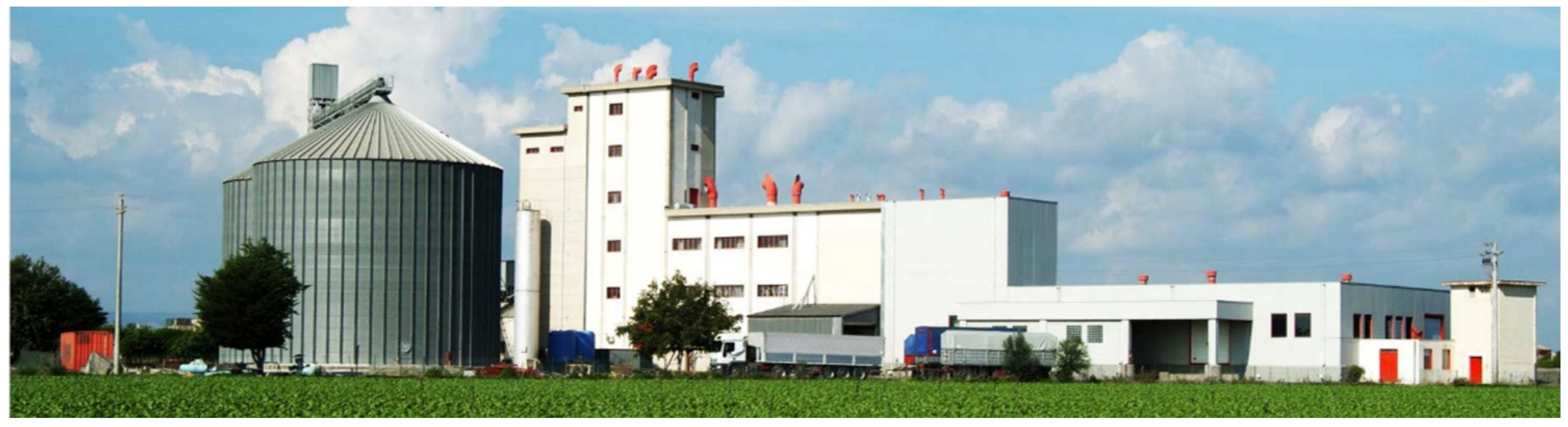
The flour mill analysed in this study is located in the province of Syracuse, in eastern Sicily (36°59′56.8′′ N, 15°13′59.5′′ E), and was built in the 1980s. The flour mill produces more than thirty products, such as biscuit flour, professional pizza mixers, and bakery improvers.

The plan of the mill is approximately rectangular, with a longitudinal axis oriented in the east–west direction. The mill has five floors, for a total height of 26.1 m (Figure 1).

The production environments, distributed over five floors, are partly intended for grain processing and partly for serving rooms (offices, laboratories, etc.) and storage of the product, which is then worked and finished.

The different floors are connected by a reinforced concrete staircase and an elevator cage. The rooms used for grain processing have a reinforced concrete frame and insulated brick walls. The floors have cavities that allow the passage of the product from a floor to another as often done in building with the same intended use [22].

2.2. The Heat Treatment

The heat treatment consists in increasing the air temperature of the treated environment until it reaches 45–55 °C, and maintaining it for 36–48 h [7,9,23,24,25]. In this study, the temperature increase was obtained by fan heaters, which allow heat distribution in the treated environment [9]. Typically, the desired temperatures are not easily reached near the floors and in the wall-to-wall and floor-to-floor intersections [1,9], which are considered “weak points” of the treatment [26].

The heat treatment of the mill was carried out by a specialised company on April 2014, and lasted 48 h, i.e., from 4:00 p.m. of 24 April 2014 to 4:00 p.m. of 26 April 2014.

The monitoring was carried out at the second floor, where the presence of the plan sifters, which are equipment sensitive to high temperatures, would make the heat treatment more damaging. However, the effect of the heat treatment on the machinery was not a direct objective of this study. The focus, instead, was on building a model suitable for simulating the air velocity and temperature fields in view of improving the technique and, by optimising the temperature distribution, the risk of damaging the machinery of the mill would be consequently reduced.

In this floor, three fan heaters were placed by the operators of the specialised company. During the treatment, the fan heaters were set to produce an output temperature of 70 °C and a volumetric flow rate of 2500 m³ h⁻¹.

2.3. CFD Analysis

2.3.1. Governing Equations and Theory behind the Model

The equations that govern fluid mechanics and heat transfer—i.e., the continuity equation, the momentum equations, and the energy equation—can be considered as the mathematical formulation of the laws of conservation governing the fluids, the heat transfer, and each phenomenon associated with them [27]. These equations are applicable in the cases of both laminar and turbulent flows, which depend on the trajectory of particles, whether uniform and parallel or not, respectively.

In this research, Autodesk^® CFD 2016 software (2016 Autodesk Inc., San Rafael, CA, USA) was used to study the indoor temperature distribution of the flour mill during the heat treatment. In the case of turbulent flow, as it is in this study, the software solves the time-averaged governing equations, obtained assuming that dependent variables can be represented by the sum of the average value and the floating value around the average.

By assuming that uppercase letters represent the mean value and lowercase letters represent the fluctuating value for the velocity components and pressure, the governing equations can be written as reported below.

• The Continuity equation, which states that the amount of entering fluid balances exactly the amount of leaving fluid, is represented by the following Equation:

  $$\frac{\delta \rho }{\delta t}+\frac{\delta \rho u}{\delta x}+\frac{\delta \rho v}{\delta y}+\frac{\delta \rho w}{\delta z}=0$$

  (1)

  where ρ is the fluid density, t is the time, and u, v, z are the velocity components along x, y, and z Cartesian axes, respectively.
• The Momentum equations, which represent the mathematical formulation of the conservation principles of the momentum and differ according to the direction, are valid for a generic x axis:

  $$\begin{gathered} \rho \frac{\delta U}{\delta t}+\rho U\frac{\delta U}{\delta x}+\rho V\frac{\delta U}{\delta y}+\rho W\frac{\delta U}{\delta z}=\rho g_X-\frac{\delta P}{\delta x}+S_{DR}+ \\ {S}_{\omega }+\frac{\delta }{\delta x}\left[2\mathsf{\mu }\frac{\delta U}{\delta x}-\rho uu\right]+\frac{\delta }{\delta y}\left[\mathsf{\mu }\left(\frac{\delta U}{\delta y}+\frac{\delta V}{\delta x}\right)-\rho uv\right]+ \\ \frac{\delta }{\delta z}\left[\mathsf{\mu }\left(\frac{\delta U}{\delta z}+\frac{\delta W}{\delta x}\right)-\rho uw\right] \end{gathered}$$

  (2)

  The term S_ω represents the rotating flow, which can be generally written as

  $$S_{\omega }=-2\rho {\omega }_i\times V_i-\rho {\omega }_i\times {\omega }_i\times r_i$$

  (3)

  where i indicates the global coordinate, ω_i is the rotational speed, V_i represents the corresponding fluid velocity component, and r_i is the corresponding distance from the rotation axis.
  S_DR represents the distributed resistance, which can be generally written as

  $$S_{DR}=-\left(K_i+\frac{f}{D_H}\right)\frac{\rho {V_i}^2}{2}-C\mathsf{\mu }{V}_i$$

  (4)

  where K is a factor that can be determined from measurements of pressure drop versus flow rate, f is the friction factor, D_H is the hydraulic diameter, and C is the viscosity coefficient.
• The Energy equation, which can be written, for incompressible flow, in terms of static temperature T, is as follows:

  $$\begin{gathered} \rho C_p\frac{\delta T}{\delta t}+\rho C_{p}U\frac{\delta T}{\delta x}+\rho C_{p}V\frac{\delta T}{\delta y}+\rho C_{p}W\frac{\delta T}{\delta z} \\ =\frac{\delta }{\delta x}\left[k\frac{\delta T}{\delta x}-\rho C_{p}uT\right]+\frac{\delta }{\delta y}\left[k\frac{\delta T}{\delta y}-\rho C_{p}vT\right]+\frac{\delta }{\delta z}\left[k\frac{\delta T}{\delta z}-\rho C_{p}wT\right]+q_V \end{gathered}$$

  (5)

  where C_p is the constant pressure specific heat, k is the thermal conductivity, and q_V is the volumetric heat source.

In the analysed model, forced convection was considered; this is a mechanism of thermal exchange that occurs when fluid currents are artificially induced by the use of an external mechanical agent, such as a heater. In forced convection flows, the temperature is influenced by the fluid motion, whereas gravity has limited or no effect.

Autodesk^® CFD 2016 uses a finite element approach (FEM) for model resolution. This approach, in its current form, consists in obtaining an approximate solution to the problem by reducing the governing partial differential equations (pdes) to a set of algebraic equations.

The elaboration of a CFD analysis with the use of software based on a FEM approach involves three subsequent steps: data pre-processing, calculation, and post-processing. The first and third steps involve the direct intervention of the user, while the second provides for no or limited operation of the user [28].

The pre-processing phase consists in dividing the object into a mesh of finite elements, and the definition of the geometry data of the model, the physical parameters of both the object and the surrounding environment (boundary conditions), and the properties of the materials constituting the model. The accuracy in the choice of parameters and the level of detail used can greatly affect the precision of the resulting simulation [28,29]. The results refer to each element involved in the simulation and each point of the model, where variables, such as temperature and speed, are computed.

The post-processing phase, instead, consists in analysing the results, selected according to the requirements, and provided by the program in the form of downloadable reports.

2.3.2. 3D Modelling

The three-dimensional model of the flour mill, where the thermal conditions were monitored, was built by using Autodesk^® Autocad 2016 software (2016 Autodesk Inc., San Rafael, CA, USA). The model was checked for “geometric inconsistencies” between component parts, such as discontinuities or intersections.

In this modelling phase, the following elements were simulated:

• components of the building, such as supporting frame, walls, floors, and windows;
• the geometric volumes of the machinery inside the considered environment;
• the position, orientation, and total number of fan heaters placed on the floor during the heat treatment;
• the volume of outdoor and indoor air.

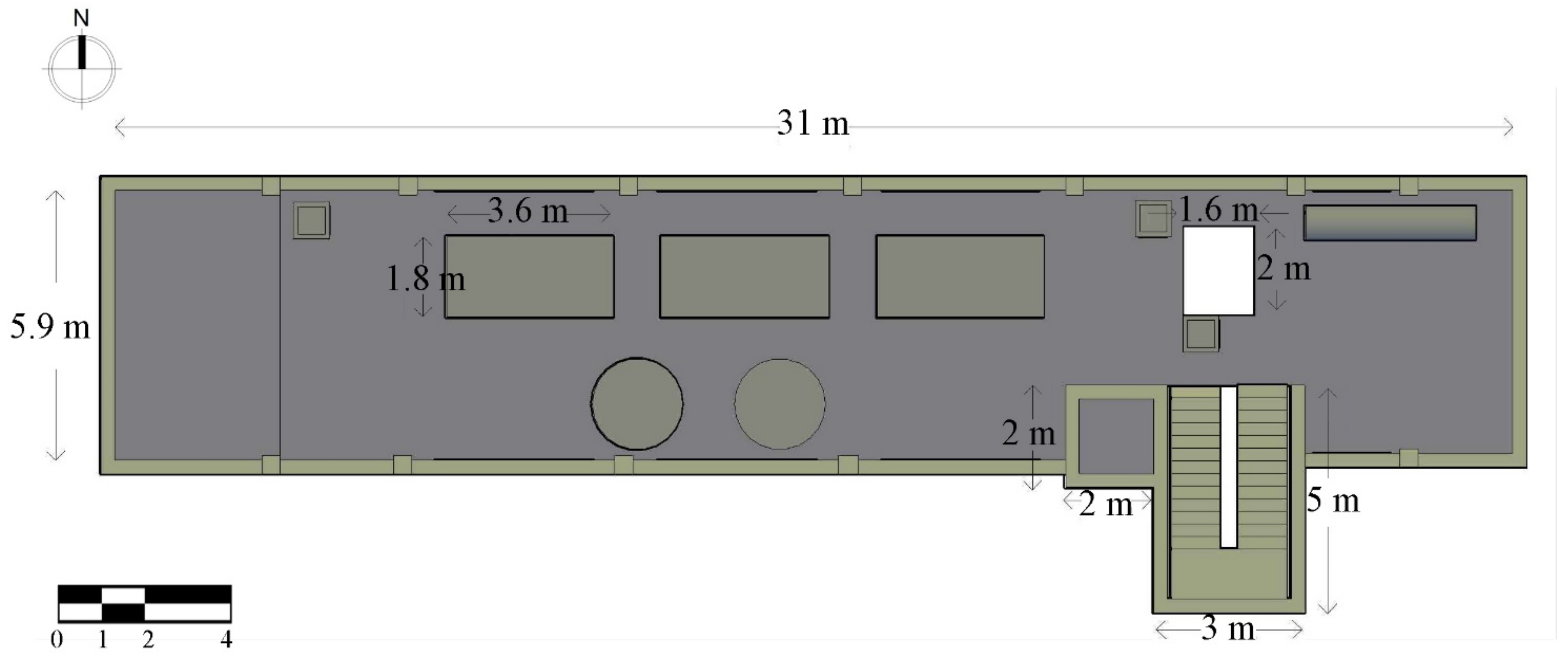
The interior dimensions of the considered floor were 31 m × 6 m × 4.8 m (Figure 2).

Each element was modelled as having the dimensions measured during the survey: the pillar section was 0.4 m × 0.4 m, the walls had a thickness of 0.3 m, while for the lower and upper floors, the thickness was equal to 0.2 m, and the windows were 1.2 m × 3.5 m (located at a height of 1.5 m from the floor). Both floors were drilled with cavities having an area of 3.8 m².

Machinery had different sizes, which reached 2 m in width, 4 m in length, and 3.8 m in height, while the size of the three fan heaters used for the heat treatment was 0.8 m × 0.8 m × 1.3 m.

The air inside the building, the fan heaters, the machinery, and the outdoor air were modelled as a volume, in order to be imported into Autodesk^® CFD 2016.

The level of detail of the 3D model allowed by Autodesk^® Autocad 2016 was considerably high compared to other tools included in CFD software (e.g., CFD2000), however, it does not include the thermal and material properties of the building components and the machinery. These properties were then assigned in the Autodesk^® CFD 2016 software.

In the modelling phase, approximations were also made for the machinery that was defined as simplified volumes, such as parallelepipeds and cylinders.

2.3.3. CFD Modelling

The 3D model designed by Autodesk^® Autocad 2016 was imported into Autodesk^® CFD 2016, where CFD simulations were performed. In the following subsections, the assignment of properties to the materials composing the building, as well as the settings of mesh size, boundary conditions, and solver parameters, are described in detail.

Materials Proprieties

At a preliminary stage, the material properties were chosen from the specific modelling editor available in the software, e.g., brick for walls and floors, concrete for frame, simple glass for windows, and steel for machinery.

The properties of the materials were partially replaced to make them more similar to the real ones by using data acquired during the survey (i.e., type of material and related thickness), bibliographic research related to similar constructions, and TerMus-PT Software (Acca Software S.p.A., Montella (AV), Italy) simulations. For concrete, only the value of thermal conductivity k (Wm⁻¹ K⁻¹) was modified. With regard to external walls and floors, instead, the modification of k required a more in-depth calculation. In fact, the software allows for assigning the material to a solid, not to a layered body. Therefore, the calculation of the thermal conductivity of the external walls and floors was carried out by using TerMus-PT software and literature data.

By using the thicknesses d and the conductivity k of the materials, which constituted the layers of external walls and floors, the thermal resistance R (m² KW⁻¹) and, subsequently, the thermal conductivity k of walls and floors were computed by the relation

$$R=R_1+R_2+\dots +R_n=\frac{d_1}{k_1}+\frac{d_2}{k_2}+\dots +\frac{d_n}{k_n}$$

(6)

The value of the thermal conductivity available in the software tool was then substituted with that computed according to the procedure outlined.

Table 1. Thickness and conductivity of the materials constituting the building components.

		Material	Thicknesses d	Conductivity k
			[m]	[Wm−1 K−1]
Building Components	Walls Thickness: 0.3 m	Concrete	-	1.01
		Internal plaster	0.02	0.60
		Brick	0.08	0.35
		Insulation	0.06	0.09
		Brick	0.12	0.35
		External plaster	0.02	0.75
	Floors Thickness: 0.2 m	Flooring	0.025	1.00
		Screed	0.035	1.10
		Hollow-core concrete roofs	0.12	0.46
		Internal plaster	0.02	0.60

shows the thicknesses d and the conductivity k of wall and floor materials. The values adopted were acquired from the general catalogues of each producer according to the values reported in ASHRAE Handbook [30]. By applying TerMus-PT software, the obtained conductivities of walls and floors were 0.534 Wm⁻¹ K⁻¹ and 0.231 Wm⁻¹ K⁻¹, respectively.

In

Table 2. Conductivity of materials used in the model.

Materials and Components	Conductivity (x, y and z)
	[Wm−1 K−1]
Air	0.026
Glass	0.780
Steel	Linear relations with T

, the conductivities of other materials used in the model are reported. They were acquired from the database included in Autodesk^® CFD 2016 software.

Meshing

In a first step of the pre-processing phase, Autodesk^® CFD 2016 divides the object into finite elements, during a process that is named discretisation or meshing, by using the finite element approach. This process leads to the design of meshes, i.e., elements constituted by nodes and rods, typically of tetrahedral shape in the case of 3D models. The calculation—today highly automated by algorithms incorporated into the software [28]—is executed at nodes, and involves different computational costs, depending on the desired detail.

In this study, the domain of the three-dimensional model has been discretised by the automatic mesh sizing, using the appropriate Autodesk^® CFD 2016 tool. With this process, the geometry was entirely evaluated, and the tetrahedral meshes were automatically built on each edge, surface, and volume of the template.

The parameters in the automatic mesh sizing tool included the following set, which were given default values:

• resolution factor, a parameter relative to the quality of the mesh in relation to model curves, equal to 1;
• edge growth rate, a parameter related to the quality of distribution computed by automatic mesh sizing, equal to 1.1;
• minimum points on edge, a parameter that guarantees a minimum level of resolution at non-curved elements, equal to 1.1;
• points on longest edge, a parameter that fixes the minimum number of points on the longest edge in the model, equal to 10;
• surface limiting aspect ratio, a parameter that controls the proportions during the automatic mesh sizing, equal to 20.

Boundary Conditions

After the meshing phase, the boundary conditions were set to connect the model to the surrounding physical world and characterise it with the internal thermal load.

Firstly, the surface temperature of the external walls was computed by using TerMus-PT software, and set as the boundary condition. Specifically, the average outside air temperature, which was measured by a portable thermo-hygrometer, and the average air temperature within the floor, which was measured by a data-logger equipped with thermal probes, were used to obtain the external wall surface temperature by the software.

In the same way, by using TerMus-PT software, the values of average temperatures recorded in the first and third floors, together with the average air temperature within the floor, were used to compute the temperatures at the outer surface of the upper floor and at the inner surface of the lower floor.

These values were set as boundary conditions for the simulations of the volume surfaces.

At the bottom cavity, the air velocity (ms⁻¹) was measured by using a portable anemometer; its motion was naturally activated by the different air pressure between the examined floor and the lower and upper floors. This air velocity was included in the model as the air velocity of the outer surface of the air volume in correspondence of the lower cavity. At the staircase, instead, the air velocity measurement was considered unreliable because it was very variable depending on the measurement point. The measured values, however, were very low, so they were not considered.

With regard to the upper cavity and staircase, a pressure equal to 0.0 Pa was set in order to obtain an air motion going from the examined floor to the upper floor.

Finally, the average value of incoming and outgoing air temperatures (°C) and volumetric flow rate (m³ h⁻¹) of the three fan heaters located on the floor were set equal to 70 °C and 2500 m³ h⁻¹, respectively.

In this case study, the boundary conditions were set as constant and non-provisional, since they were invariable during the simulation. They defined the inputs and outputs of the model: conditions such as pressure, velocity, and volumetric flow determined the input and output paths of the fluid.

According to the forced convection field, one inlet region and two outlet regions, located at the cavities and the staircase, were defined in the model.

Solver Settings

Before starting the simulation, the following default convergence parameters were set in the software: the maximum instantaneous convergence slope, from one iteration to the next, was equal to 10⁻³; the time averaged convergence slope and the time averaged convergence concavity were both equal to 0.03162; the field variable fluctuations was equal to 10⁻⁴.

Concerning the physical characteristics of the model, the fluid was considered incompressible, and a k-ε turbulence model was applied. This model is commonly used, in fact, to represent the average characteristics of turbulent flow conditions, and is based on two transport equations. The first transport variable determines energy in turbulence and is named “turbulent kinetic energy” (k). The second transport variable determines k dissipation rate and is named “turbulent dissipation” (ε).

For coherence with physical reality, the “Heat Transfer” and “Auto Forced Convection” parameters were set to ON. In a forced convection analysis, in fact, the flow and the heat transfer can be solved separately, because the flow does not depend on the temperature distribution. By using the “Auto Forced Convection”, this procedure becomes automatic, because it involves the execution of the two-step analysis. The first phase only considers the flow (without thermal transfer), while the second one solves only for thermal transfer.

2.4. Survey of Air Temperatures for Model Assessment

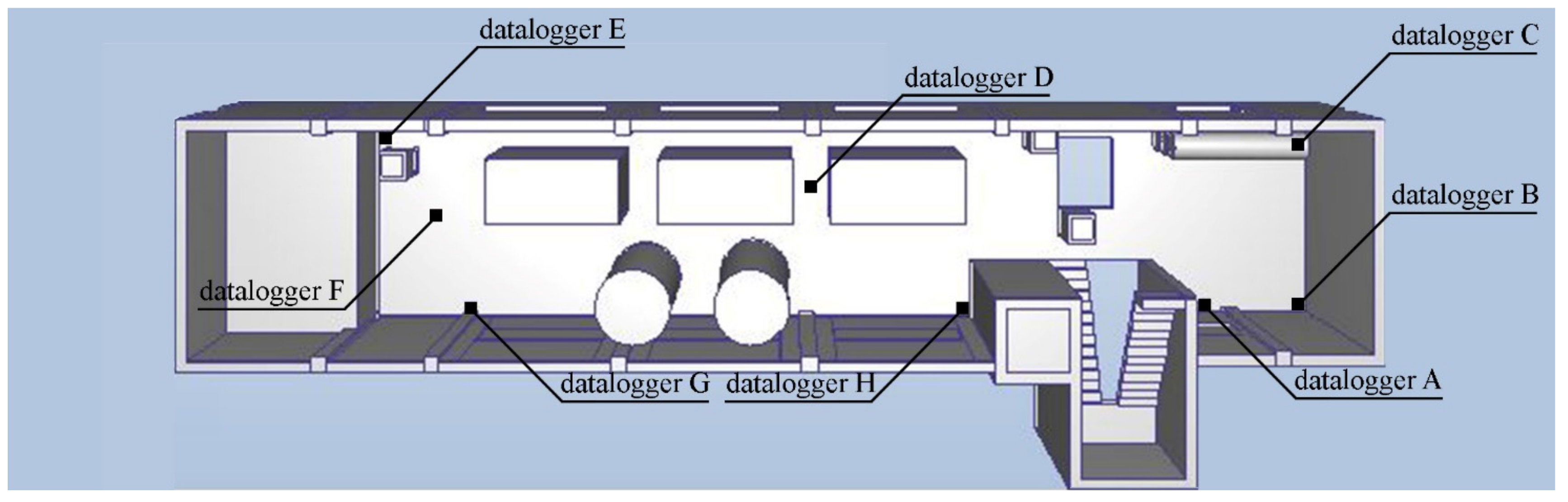
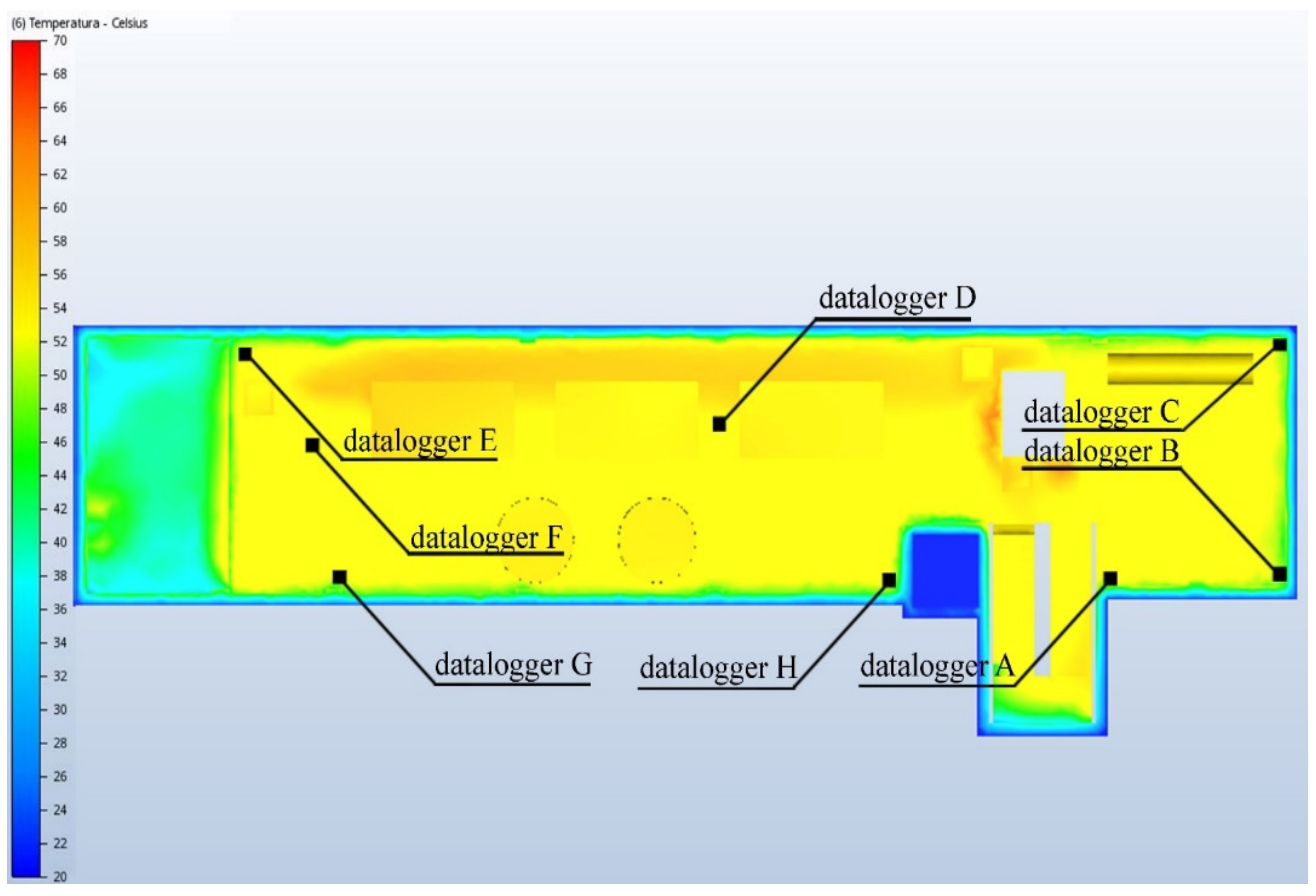
During the heat treatment, monitoring of air temperature distribution in some areas of the flour mill is crucial to achieve the efficacy of the treatment, as well as avoid damage to the equipment. Therefore, in this research study, some data-loggers were placed near building components which, as demonstrated in previous studies, reached lower levels of surface temperatures, i.e., thermal bridges [26,31] (data-loggers A–B–E–G–H); other data-loggers were placed near equipment that could be damaged during the heat treatment due to the high temperatures (data-loggers C–D). Finally, the position of data-logger F was chosen to monitor the effectiveness of the heat treatment at a distant point from both the walls and the fan heaters (Figure 3).

The positioning of these probes was made both along horizontal and vertical planes. They were placed at a height of 0.2 m, except for data-logger D, which was fixed at a height of 2.7 m.

Air temperature data in the reference floor were detected before and during the heat treatment by using eight Grillobee data-loggers manufactured by Tecnoel (Milan, Italy) connected to temperature transducers produced by Rotronic Italia s.r.l. (Milan, Italy) and placed in different points of the floor in order to obtain a uniform field of temperatures. The temperature data were sampled every 15 s and stored every 30 min, thus obtaining a total of 13 measurements in the time interval considered for each data-logger utilised in this study. The data acquisition was performed by connecting each Grillobee unit with a laptop computer through serial ports.

The monitoring of air temperature by these devices was carried out during the whole heat treatment. However, only the time interval between 12:00 a.m. of 26 April 2014 and 6:00 a.m. of the same day, which can be considered stationary, was taken as the time interval of analyses in this study. During the next hours, in fact, the company that performed the heat treatment changed position and orientation of the fan heaters, which were rotated in order to obtain a better heat distribution. This action led to a slight variation in the air temperature values recorded by the data-loggers next to the fan heaters, hence, those hours were excluded in this study.

During the survey, portable anemometers for air velocity measurement were used at the cavities. Spot measurements were carried out at fixed times during the heat treatment since indoor hygrothermal conditions are unfavourable for a long stay in this environment.

During the treatment, a thermal camera (ThermaCamB2 by FLIR System Inc., Wilsonville, OR, USA) was also used to obtain thermographic images of the internal surfaces of the building components of the thermal bridges. By using these images, the mapping of wall temperatures was carried out and utilised to perform the assessment of the model.

3. Results and Discussion

3.1. Model Assessment

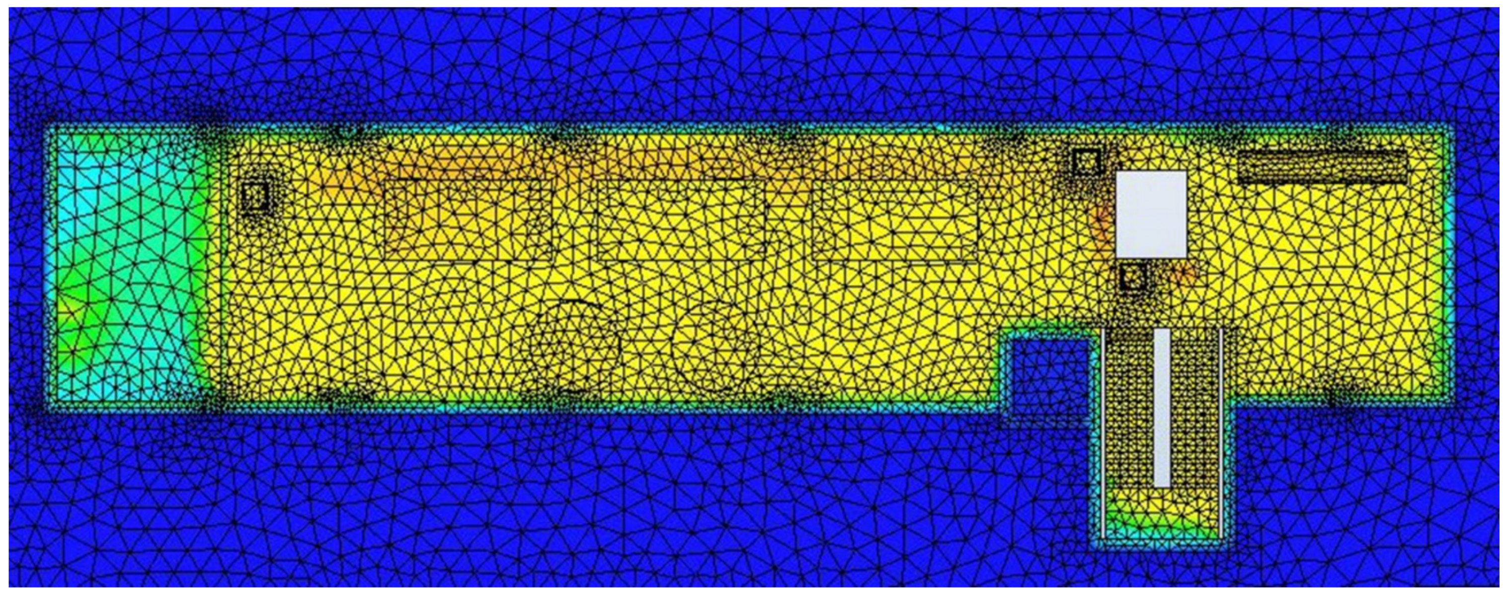
The automatic mesh sizing, used in this study, led to the creation of about 2 × 10⁵ nodes and 7.4 × 10⁵ elements (Figure 4), which allowed for a relatively quick simulation. In fact, a limited number of iterations (476) was required to achieve model convergence and resolution.

Based on the measurements collected during the surveys and the subsequent CFD simulations, several data were obtained both for the input region (Inlet 1) and the two output regions (Outlet 1 and Outlet 2), as shown in

Table 3. Characteristics of input and output regions.

Input Region (Lower Cavity)	Inlet Bulk Pressure	Inlet Bulk Temperature	Mass Flow in	Reynolds Number	Volume Flow in
Inlet 1	0.19 Nm−2	53.5 °C	15.14 kg s−1	465704.00	12.56 m3 s−1
Output Region (Upper Cavity and Staircase)	Outlet Bulk Pressure	Outlet Bulk Temperature	Mass Flow out	Reynolds Number	Volume Flow out
Outlet 1	0.00 Nm−2	52.75 °C	−3.20 kg s−1	49,556.70	−2.66 m3 s−1
Outlet 2	0.00 Nm−2	52.75 °C	−12.69 kg s−1	390,526.00	−10.54 m3 s−1

.

The bulk pressure (Nm⁻²) was positive in correspondence of the input region, because it represents an entry region of airflow. The values in correspondence of output regions were equal to 0.00 Nm⁻², as set in the CFD modelling phase.

The values of inlet and outlet bulk temperature (°C) derived from the settings of boundary conditions, as well.

With regard to the mass flow (kg s⁻¹), it was observed that most of the mass flow that comes in through inlet 1 (15.14 kg s⁻¹) comes out at outlet 2 (−12.69 kg s⁻¹), corresponding to about 84% of the flow, while only about 16% comes out at outlet 1 (−3.20 kg s⁻¹). Similarly, in relation to the volume flow (m³ s⁻¹), it is observed that most of the volume flow that comes in through inlet 1 (12.56 m³ s⁻¹) comes out at outlet 2 (−10.54 m³ s⁻¹), corresponding to about 84% of the flow as expected, while only about 16% comes out at outlet 1 (−2.66 m³ s⁻¹). This is due to the fact that the inlet 1, corresponding to the lower cavity, is exactly below the outlet 2, corresponding to the upper cavity. Therefore, this geometric configuration favours airflow through the two cavities.

The considerable airflow between the two regions is also reflected in the value of the Reynolds number, which was observed to be much greater at inlet 1 and outlet 2 (respectively equal to 465,704.0 and 390,526.0) compared to the one at outlet 1 (equal to 49,556.7).

Table 3 shows slight mass flow and volume flow imbalances, which are due to the choice of the advection scheme before starting the simulation. For this CFD analysis, advection scheme 1 (Monotone streamline upwind) was set. This is the default scheme for almost all analyses, recommended as a starting point for most types of analysis.

Additionally, an analysis using the advection scheme 5 (Modified Petrov–Galerkin) was carried out. This scheme produces more globally conservative results. Comparison of the results obtained with the use of the two alternative advection schemes is shown in

Table 4. Results obtained with the use of the advection schemes 1 and 5 in terms of mass flow balance and volume flow balance.

Advection Scheme	Mass Flow in	Mass Flow out	Volume Flow in	Volume Flow out
1 (Monotone Streamline Upwind)	15.14 kg s−1	−15.89 kg s−1	12.56 m3 s−1	−13.20 m3 s−1
5 (Modified Petrov–Galerkin)	15.14 kg s−1	−15.00 kg s−1	12.56 m3 s−1	−12.46 m3 s−1

.

By setting advection scheme 5, mass flow and volume flow imbalances decreased, whereas the difference between the temperatures measured through data-loggers and those simulated at the same points of the floor increased. This effect on temperatures between 12:00 a.m. and 6:00 a.m. on 26 April 2014 is more broadly discussed in the following section.

3.2. Analysis of the Temperatures Recorded during the Survey

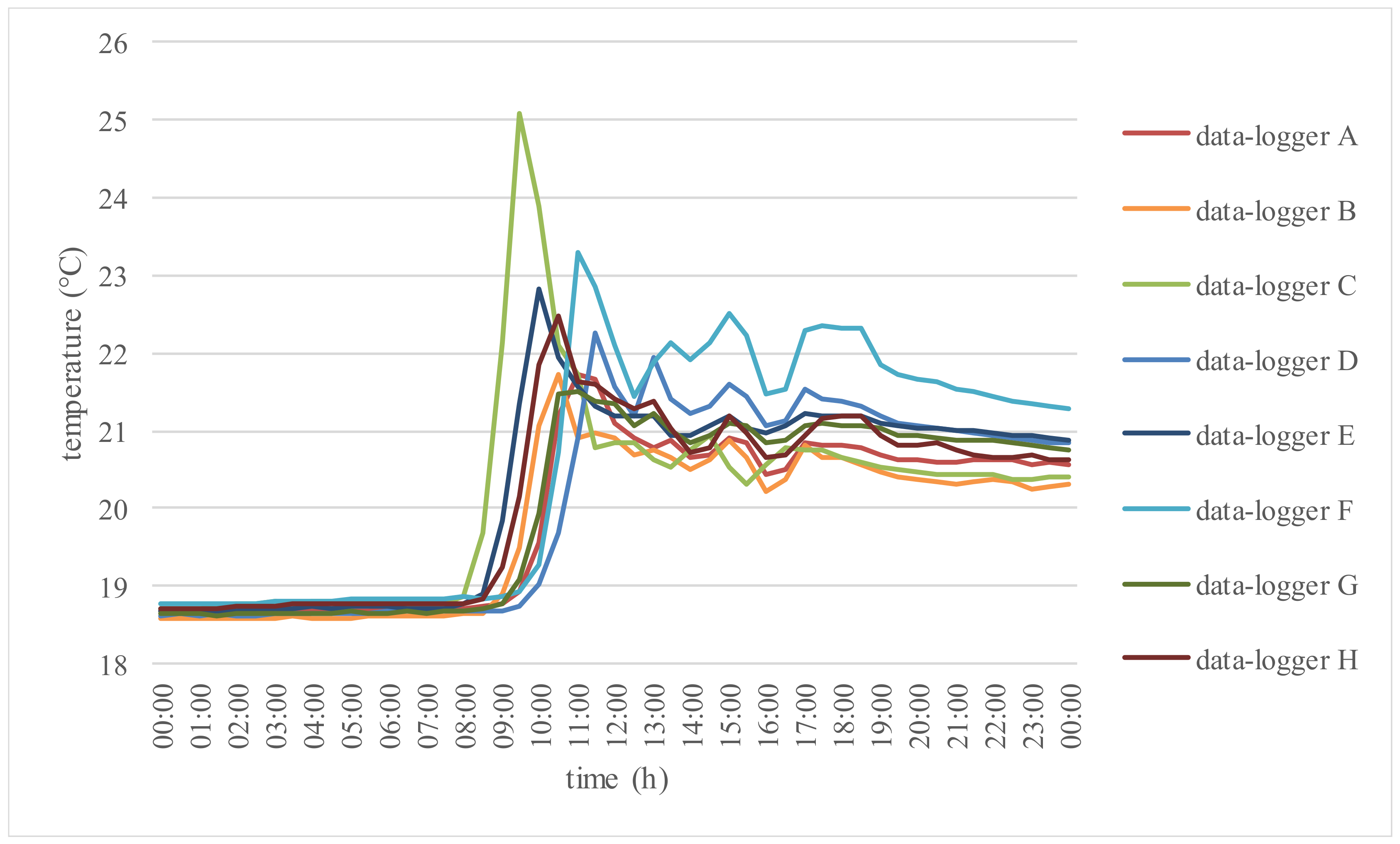
On the day before the heat treatment (23 April 2014), the average temperature recorded by the data-loggers was 20.06 °C. The highest temperature was recorded by the data-logger C, and it was equal to 25.08 °C (Figure 5).

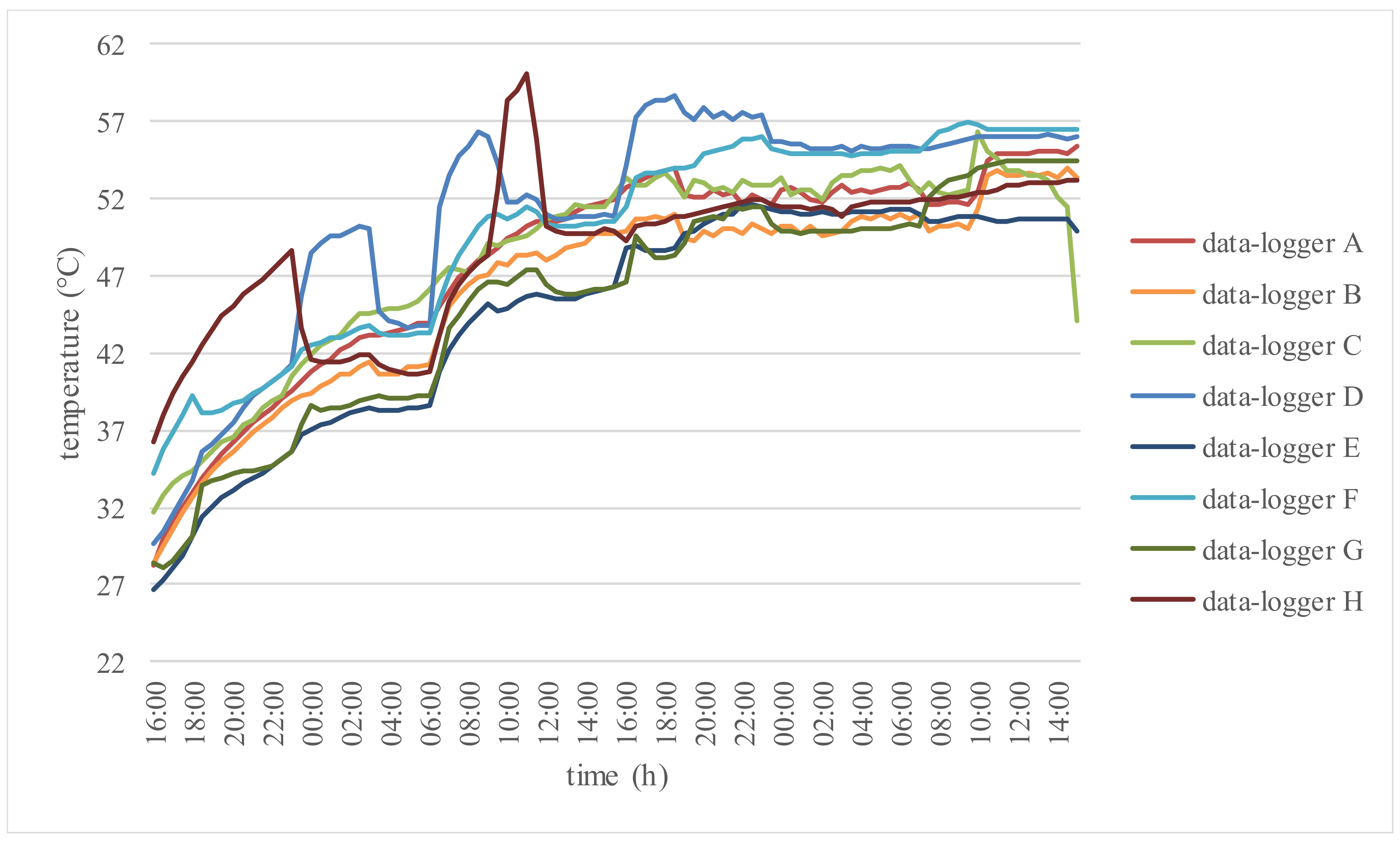
During the heat treatment, performed from 4:00 p.m. of 24 April 2014 to 4:00 p.m. of 26 April 2014, the data-loggers recorded an average temperature of 47.72 °C, with a maximum value of 60.04 °C, detected at the data-logger H, and a minimum value of 26.6 °C, detected at the data-logger E (Figure 6).

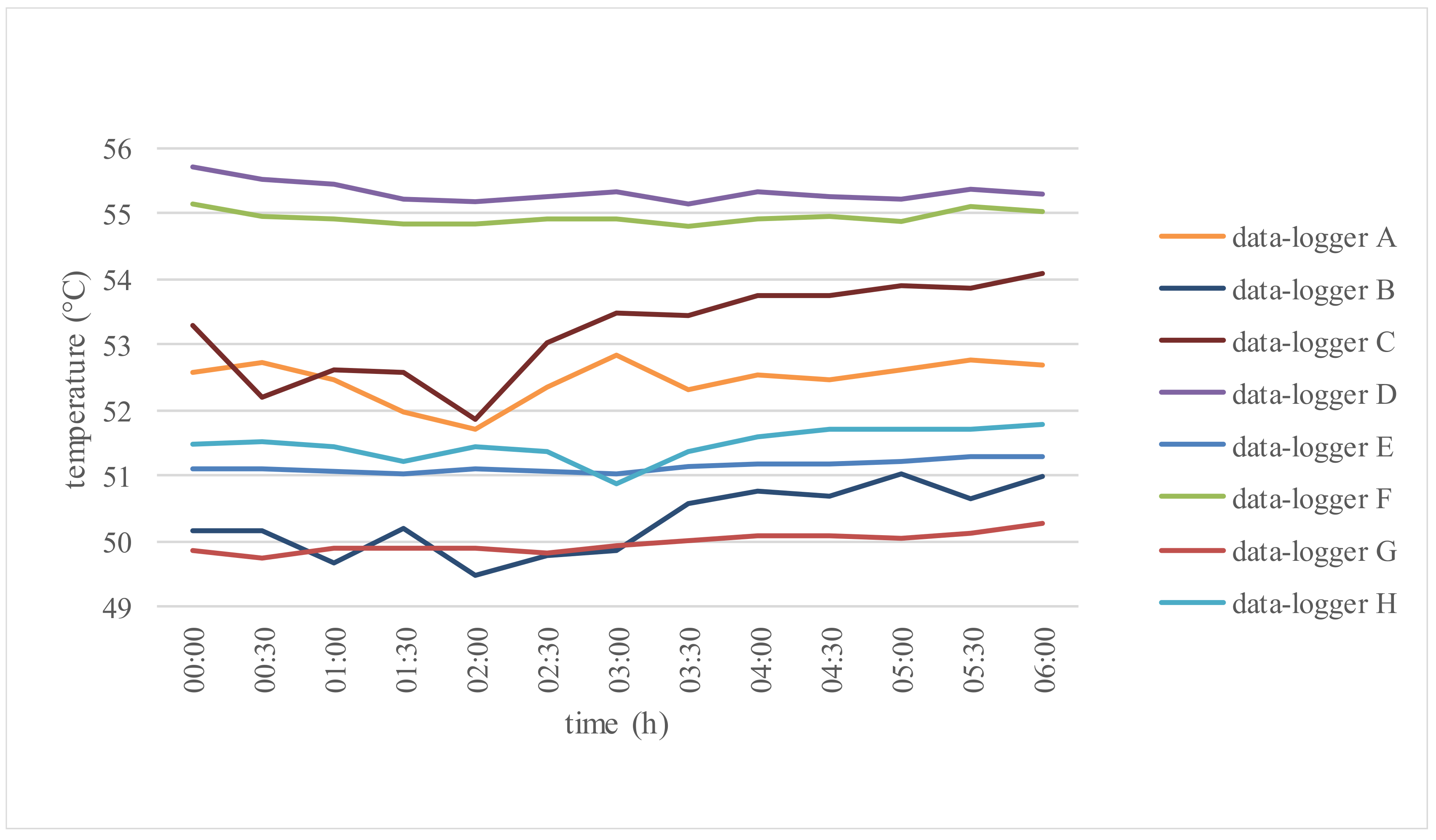
In order to perform simulations with Autodesk^® CFD 2016 software, only temperatures between 12:00 a.m. and 6:00 a.m. on 26 April 2014 were evaluated, since they can be considered quite stable with variations reaching a maximum value of 2.22 °C and an average value of 0.935 °C (Figure 7). In this period, moreover, the standard deviation reached a maximum value of 0.71 and an average value of 0.28.

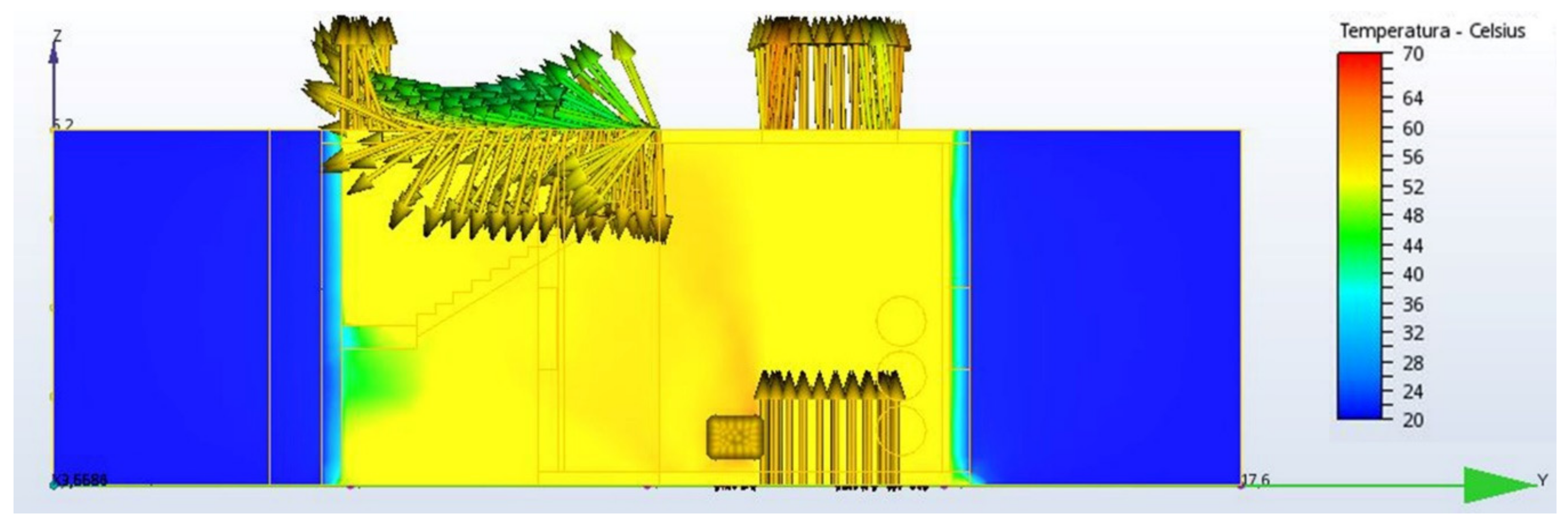
During the same time interval, the outside air temperature was about 20 °C, while the average air temperatures of the lower and upper floors were 57.3 °C and 56.4 °C, respectively. By considering these values of air temperature, surface temperature values equal to 21 ° C on the external walls, equal to 53.5 °C on the outer surface of the upper floor and equal to 52.75 °C on the inner surface of the lower floor were computed by using TerMus-PT software. Finally, an air velocity of 4 ms⁻¹ was recorded at the lower cavity (Figure 8).

3.3. Validation

In order to assess the model, the average air temperatures recorded by the data-loggers during the stationary period were compared with the temperatures obtained in the simulation at the same points within the model created with Autodesk^® CFD 2016 (Figure 9).

The model overestimated air temperature at the points where data-loggers A, B, D, E, F, G, and H were located, and the average overestimation value was equal to 1.08 °C. The maximum value of overestimation was observed for data-logger F (+2.57 °C). The model underestimated the air temperature only at the point where data-logger C was located, and the underestimation value was equal to −0.22 °C.

The relative errors were 4.57% and 0.41%, respectively. Since the relative errors were below 10%, by using a similar justification as that proposed by Zhang et al. [32], the validation of the CFD model can be considered good.

Results of comparisons between temperatures simulated by the CFD analysis and those stored by the data-loggers at the different locations surveyed are shown in

Table 5. Measured and simulated temperatures at the same points of the floor between 12:00 a.m. and 6:00 a.m. on 26 April 2014 and related temperature differences.

Data-Loggers	A	B	C	D	E	F	G	H
Simulated temperature [°C]	53.18	52.24	53.00	55.68	52.15	57.51	50.22	52.21
Measured Temperature [°C]	52.46	50.31	53.22	55.33	51.14	54.94	49.97	51.48
Δ	−0.72	−1.93	0.22	−0.35	−1.01	−2.57	−0.25	−0.73

.

3.4. Sensitivity Analysis

Although affected by the variation in the position of the portable anemometer, the air velocity survey, made at the lower cavity, returned values around 4 ms⁻¹. In order to evaluate the model accuracy, a sensitivity analysis was carried out by performing several simulations with variable values of the air velocity at the cavity. The results of this sensitivity analysis are shown in

Table 6. Measured and simulated temperatures at the same points of the floor between 12:00 a.m. and 6:00 a.m. on 26 April 2014 and related temperature differences. Sensitivity analysis with variable values of the air velocity at the lower cavity.

Air Velocity	Data-Loggers	A	B	C	D	E	F	G	H
	Simulated temperature [°C]	53.18	52.24	53.00	55.68	52.15	57.51	50.22	52.21
V = 3.0 ms−1	Measured Temperature [°C]	53.18	51.55	55.72	56.43	52.40	59.37	50.54	51.37
	Δ	0.00	0.69	−2.72	−0.75	−0.25	−1.86	−0.32	0.84
V = 3.5 ms−1	Measured Temperature [°C]	53.14	51.72	53.46	55.26	53.12	57.79	50.25	51.40
	Δ	0.04	0.52	−0.46	0.42	−0.97	−0.28	−0.03	0.81
V = 4.5 ms−1	Measured Temperature [°C]	52.77	53.27	52.71	54.65	53.57	56.56	49.09	52.23
	Δ	0.41	−1.03	0.29	1.03	−1.42	0.95	1.13	−0.02

.

The absolute value of the maximum temperature difference |Δ| was observed at the data-logger C (|Δ| = 2.72 °C) with an air velocity value equal to 3 ms⁻¹, while the minimum one was for the data-logger A (|Δ| = 0.00 °C) with a value of air velocity equal to 3 ms⁻¹. Therefore, the values observed in Table 6 showed that in most of the points where data-loggers were placed, a value of 4 ms⁻¹ was adequate for the simulation.

3.5. Wall Thermal-Camera Images Compared with Temperature Maps from CFD Simulations

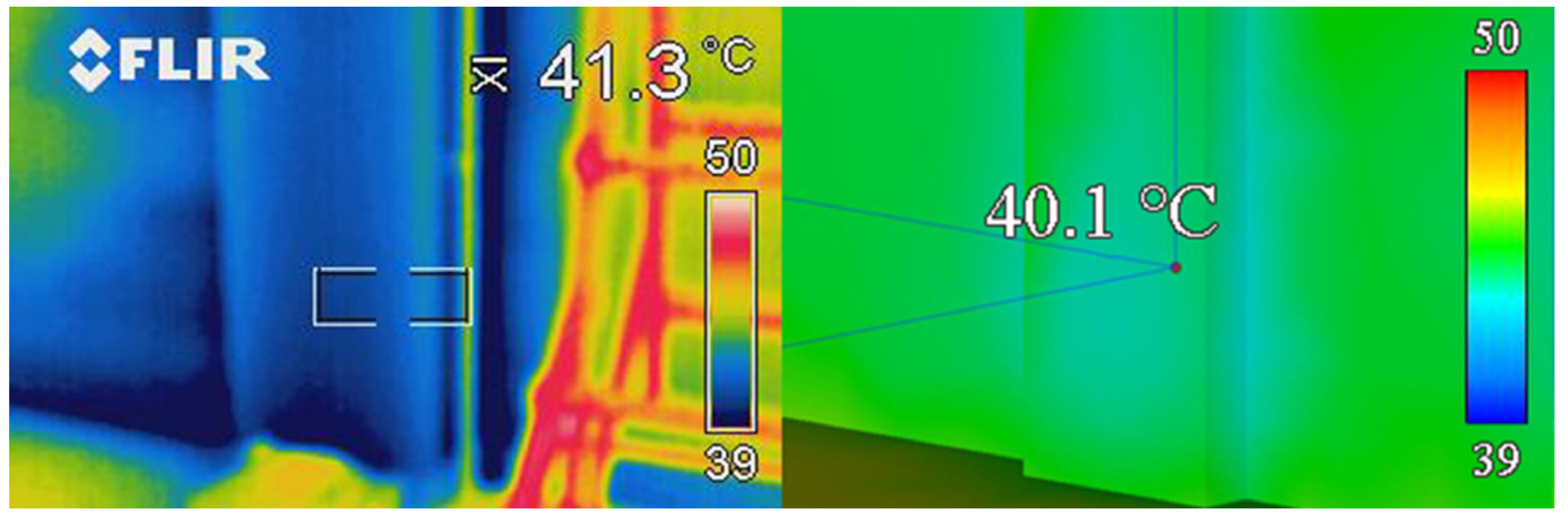
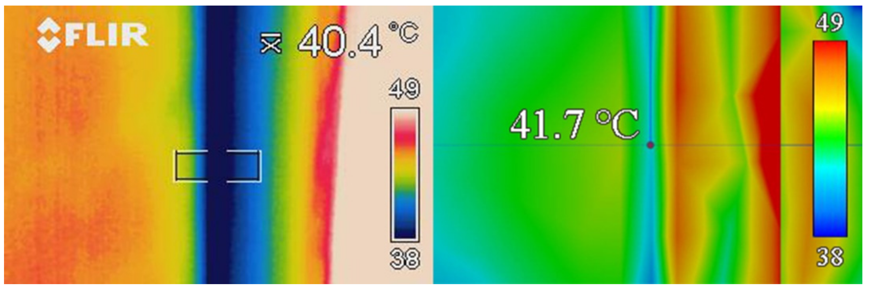
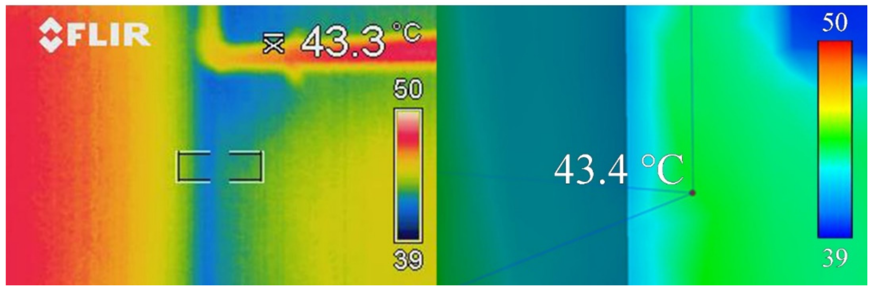
Wall temperature mapping, obtained by using the thermal camera during the considered heat treatment, was utilised in the final phase of this study for a further assessment of the model and, specifically, simulated temperature at the most relevant points on the walls (e.g., thermal bridges) were compared to the corresponding points in the thermal images.

In the images of Figure 10, Figure 11 and Figure 12, some examples of the comparisons between the measured and simulated surface temperatures at several points of the external walls and the reinforced concrete frame are reported. At these points, it was observed that the maximum value of overestimation was equal to 1.30 °C, and the maximum value of underestimation was equal to 1.20 °C.

In

Table 7. Average temperatures recorded at data-logger locations during the last 36 h of heat treatment.

Data-Logger	A	B	C	D	E	F	G	H
Measured Temperature [°C]	51.15	49.17	51.34	54.12	47.94	52.75	48.68	50.42

, the values of the average indoor air temperatures measured during the last 36 h of heat treatment are shown. Although the average indoor air temperatures recorded were above 47 °C (Table 7), however, from the images detected by the thermal camera at the thermal bridges, it was observed that the surface temperatures were much lower than 45 °C, which is the threshold value for the success of the heat treatment [7,23,25,26]. Therefore, building interventions are crucial to improve building thermal performance during heat treatment, as it was suggested in previous studies [26,31].

The main activity of this research was to assess temperature distribution inside a flour mill during a heat treatment for insect pest control by computational fluid dynamics (CFD) modelling and simulation. Since the CFD model of this research study made it possible to obtain a temperature distribution that fitted the real one with a good accuracy, further improvements could be planned, for instance, by using manual meshing to apply finer sizes to selected surfaces and edges of the model, in order to capture strong flow gradients or represent complicated geometric features.

The CFD model, designed in this study, could be used to improve the efficiency of the heating system by modifying number, power, and position of fan heaters, which are usually empirically chosen by heat treatment operators without specific planning. In particular, CFD simulations should be carried out by changing the position and/or the rotation of the fan heaters in order to obtain a more uniform distribution of the indoor temperature values close to those lethal to insects. To this end, a further study is in progress, and will be subject of a following paper.

Furthermore, the CFD model could be used to choose building interventions suitable to improve thermal performance of the building envelope. They may involve wall-layer modifications, with particular attention to the type of insulation adopted and the related thickness [31,33,34,35] or wall-openings shielding, by adopting sheets able to reflect the thermal radiation.

4. Conclusions

The main objective of this study was defined based on the evidence derived from research studies reported in the literature, which showed the need for developing a model suitable to select the most appropriate strategy for treatment optimisation and minimisation of energy costs, which economically affect treatment execution and sustainability. Therefore, this objective was achieved in this study by developing a CFD model, which gives a realistic representation of the inner conditions of the mill and, in general, of the thermal behaviour of the building. Air temperatures and air velocities in the indoor environment were recorded by using data-loggers and portable anemometers, and integrated by the measure of values related to the external environment. The data-loggers were located to monitor the air temperature distribution in those areas of the flour mill that are crucial for the treatment efficacy, i.e., areas close to thermal bridges, which reached lower levels of surface temperatures, and areas close to equipment that could be damaged during the heat treatment, due to the high temperatures.

For this purpose, a 3D model was made by using the Autodesk^® Autocad 2016 software, then it was imported into Autodesk^® CFD 2016 and completed with the information needed to perform the CFD analysis, such as materials and boundary conditions. After performing the discretisation of the domain, simulations were conducted in order to obtain the distribution of the internal temperature values.

As shown by the comparison between temperatures measured by data-loggers and temperatures obtained at the same points within CFD simulations, the model succeeded in representing the thermal conditions of the indoor environment during the heat treatment. Therefore, the method described in this study could be followed for the modelling and simulation of the thermal behaviour of other flour mills during the heat treatment for insect pest control.

This result is of significant importance in view of optimising the heat treatment procedure, by changing fan heaters’ configuration to obtain a more uniform distribution of the indoor temperature values, or by improving the thermal performance of the building envelope through suitable building interventions.