1. Introduction
The design of buildings where daylight is utilized to illuminate building interiors is becoming more commonplace today as green building rating systems, energy codes, and standards are promoting or requiring the introduction of more daylight [
1,
2,
3,
4,
5]. Some now require the installation of automatic photocontrol of electric lighting in daylight zones that are adjacent to windows and under skylighting systems. Research has shown that installed photocontrolled electric lighting systems frequently do not operate in an ideal manner due to product performance limitations, system layout, or poor calibration [
6]. Poor performance can lead to dissatisfied occupants, complaints, dismantling of the system, and a loss of energy savings.
This paper discusses how the design and layout of these systems can be aided through detailed computer modeling that accounts for the following real world conditions: local weather, reflections and shadows from the exterior surround, space and daylight aperture geometry and materials, operable shading devices, and the layout and relevant performance features of the electric lighting and lighting control systems. With this wide range of inputs, daylight-integrated lighting control system modeling is a complex problem. At least two software tools are now available that provide packaged modeling capabilities that enable a designer or manufacturer to make informed decisions related to product selection, layout, and overall system design. SPOT [
7,
8] and DAYSIMps [
9,
10] are the two major photocontrol system simulation tools that are available for free from their respective websites. Each makes use of the Lawrence Berkeley Laboratory
Radiance software developed by Ward [
11,
12].
This paper summarizes a number of design and analysis features that are included in these tools, or that have been addressed in research papers and are likely to appear in these or similar tools in the future. The topics include the range of inputs that must be addressed, the analysis methods that can be applied, and the different metrics and methods for displaying, assimilating, and assessing the resulting performance data. More widespread application of these resources to the design and analysis of these products and systems should lead to a better understanding of their performance, as well as improvements in their overall effectiveness. These improvements should lead to increased occupant acceptance of these systems and significant reductions in lighting energy consumption in both new construction and retrofit applications.
2. Simulation Methods and Calculations
2.1. Illuminance Calculations
Daylighting calculations that cover time intervals across an entire year are typically performed using a single daylight coefficient or a multi-step matrix approach, applying either three or five calculation phases with bidirectional scattering distribution functions (BSDFs) to quantify light transmission through complex fenestration systems. These approaches permit relatively simple calculations to be performed for each time period following a detailed initial analysis to compute the daylight coefficients or matrices. In both of these methods, the sky is discretized into a large number of patches (from hundreds to thousands of angular regions across the sky hemisphere). The luminance of each sky patch at each time interval is typically determined using Perez skies, which are formulated from the hourly solar and global irradiance data contained within a .tmy or .epw site weather file.
2.1.1. Single-Phase Daylight Coefficients
Single phase daylight coefficients are multiplying factors that relate the luminance of each of these patches to the illuminance at an interior analysis point, or to a photosensor signal. This approach simplifies the analysis of sky conditions across the year to a simple matrix multiplication that considers daylight coefficients and sky luminance values at the provided simulation times across the year. If different shade settings must be considered, a new set of coefficients must be computed for each shade setting. The values at each hour of the year are then compiled based on the shade settings applied at each hour. The reading of a photosensor’s signal can be determined by applying its spatial sensitivity for each of the incoming light rays when computing its set of daylight coefficients.
2.1.2. Multi-Phase Approach
The multi-phase BSDF approach applies a series of matrices that consider the daylight as it passes through different segments along the path from source to analysis point. In a typical implementation, a daylight matrix quantifies the amount of light arriving at different input directions on the exterior of a complex fenestration system based on daylight source location (for the sky patches and sun locations). This matrix accounts for exterior reflections from the ground plane as well as any other exterior surfaces that are included in the model. Next, a BSDF matrix quantifies the redirection of this light as it passes through the complex fenestration system (CFS), which can be comprised of fabric shades, slatted blinds, or a specular louver system, or it might simply consider the transmission of daylight through a clear or translucent window material. For every incoming ray direction to the CFS, there is a set of coefficients that describes the amount of light redirected in each outgoing angle. Finally, a view matrix relates the interior illuminance at a point, or the signal received at a photosensor, to the light that is emitted in various directions from the inside surface of the CFS.
2.1.3. Direct Sunlight Contribution
In either of the above approaches, the contribution from the sun may be integrated into the sky patches or separately determined. In its simplest form, the sun’s contribution is applied to a single patch, but another approach distributes it across three sky patches [
13]. For more accurate results, the direct sunlight contribution can be separately calculated after subtracting out the sun’s direct contribution from these patches to the analysis points, leaving the reflected component for the sun to be considered using sky patch coefficients. The direct contribution is then recomputed using appropriately sized and positioned solar disks to provide more accurate modeling of the location of the penetrating solar beam. Since only the direct contribution is recalculated in this approach, this enhanced calculation requires little additional processing time and improves the placement of sunlight patterns within a space. Accurate sunlight patterns are required for the calculation of metrics such as annual sunlight exposure (ASE) and for controlling shades when assessing spatial daylight autonomy (sDA) [
14]. These recently developed metrics can be utilized to qualify a building for daylight credits in LEED V4 [
5]. With the Radiance programs that are applied in this five-phase approach, the direct sun calculation can even consider the direct sunlight that passes through a series of blind slats by applying a proxy geometry to a BSDF material, where object geometry is considered when computing the direct component [
15]. In this setup, the BSDF is still used to determine the interior reflected contribution from direct sunlight that enters a space and for the analysis of both the sky and ground contributions to the building interior.
2.2. Shading Device Operation
In order to properly assess the energy savings achieved with daylight-integrated electric lighting control, the operation of any shading devices at the window apertures must be assessed. Different blind angles and shading device lowering positions can be considered using either available BSDF data or through physical modeling of the blind or shade materials and their geometry.
Shading device activation is generally automated within annual simulation daylight analysis software, with the shade device setting governed by a photosensor signal, solar position, glare calculations, solar gain, or some combination of these. If shades are to be controlled by the occupant, which is common in most buildings, then a statistical algorithm based on typical user behavior can be applied [
16]. A statistical approach that attempts to predict how occupants control their shades will likely provide a range of settings across different spaces on a façade, and across similar sky conditions, based on research findings.
2.3. Energy Savings Calculations
2.3.1. A Simplified Approach
In assessing the potential energy savings that can be achieved with an integrated electric lighting control system, a range of different approaches, which consider different user inputs, are available. For example, in the EnergyPlus whole building energy modeling software, daylight-integrated lighting control is assessed by indicating the following: the space lighting power density, the fraction of the lighting system that is controlled, and the location of a reference point and target illuminance that governs the controlled zone’s dimming level [
17]. The challenge with this approach involves the proper location of the reference point and the correct specification of its target illuminance level. For best results, the reference point should be located at the critical work plane position which, for most hours of the year, would dictate the desired output from the controlled lighting zone.
When specifying the target illuminance for the reference point, the user must consider the fact that non-controlled electric light might also be present at that task location. For example, if 400 lux is the total illuminance that is to be maintained at all possible work locations within a classroom, proper control may require the controlled lighting zone to be dimmed to minimum output when only 250 lux of daylight is received at the critical point, if 150 lux is produced at this point from an interior lighting zone that is not dimmed.
In a private office, it might be possible to identify the desk location and locate the reference point upon this desk. In a classroom, however, the location of the critical point on the work plane—the point that requires the highest light output setting from the controlled lighting zone—is somewhere across a large area. Its location is based on features of the electric lighting system, including the layout of the controlled zone and the luminaire photometry, as well as the daylight distribution within the space. In the case of a tool such as EnergyPlus, the dimmed lighting zone is typically entered as a fraction of the room area. If the portion of the electric lighting system being dimmed is aligned with the area of the room that receives maximum daylight, it should be possible to estimate where the reference point is likely to be positioned. An algorithm that conducts an analysis to select this point, rather than requiring the user to guess at its location, would offer a more consistent and accurate approach for a simplified energy analysis, particularly for users who have a limited understanding of photocontrol system modeling.
2.3.2. A Detailed Approach
In a more advanced energy or control system analysis, the complete electric lighting system can be specified, with luminaire photometric distributions provided through IES or LDT photometry files [
18,
19]. Control zones that are configured in accordance with daylight zones described in an energy code, or that align with the areas of the room that consistently register high levels of daylight (easily quantified using a metric such as daylight autonomy), can then be specified. Electric light contributions are then computed separately for the dimmed and non-dimmed zones, along with the daylight contribution, at each point. With these values, it is then possible to determine an appropriate dimming level for the electric lighting system at each daylight interval across the year.
where
is the total illuminance,
is the target illuminance,
is the daylight illuminance at the calculation point,
is the dimming level required to maintain the target illuminance,
is the illuminance contribution from the non-dimmed zone at the calculation point, and
is the illuminance contribution from the dimmed zone at the calculation point.
This process can be evaluated at all points or applied to only one or more “critical points” [
20] across the work plane. In applying this approach to a critical point, if the point receives more electric light than is required to meet the target illuminance at night, calibration of the photosensor may also result in energy savings at non-daylight conditions due to task-level tuning. Some tools may permit this energy to be separately quantified from that which results from daylight-integrated control alone. It is important when calibrating the lighting control system to only permit task-level tuning to occur if it will occur in the real space, and verify that no other task location requires a higher light output level at night than the output level specified by the critical point(s). An appropriate light loss factor should be included in the electric lighting system calculations when applying this approach.
2.4. Critical Point Determination
2.4.1. Automatic Assessment
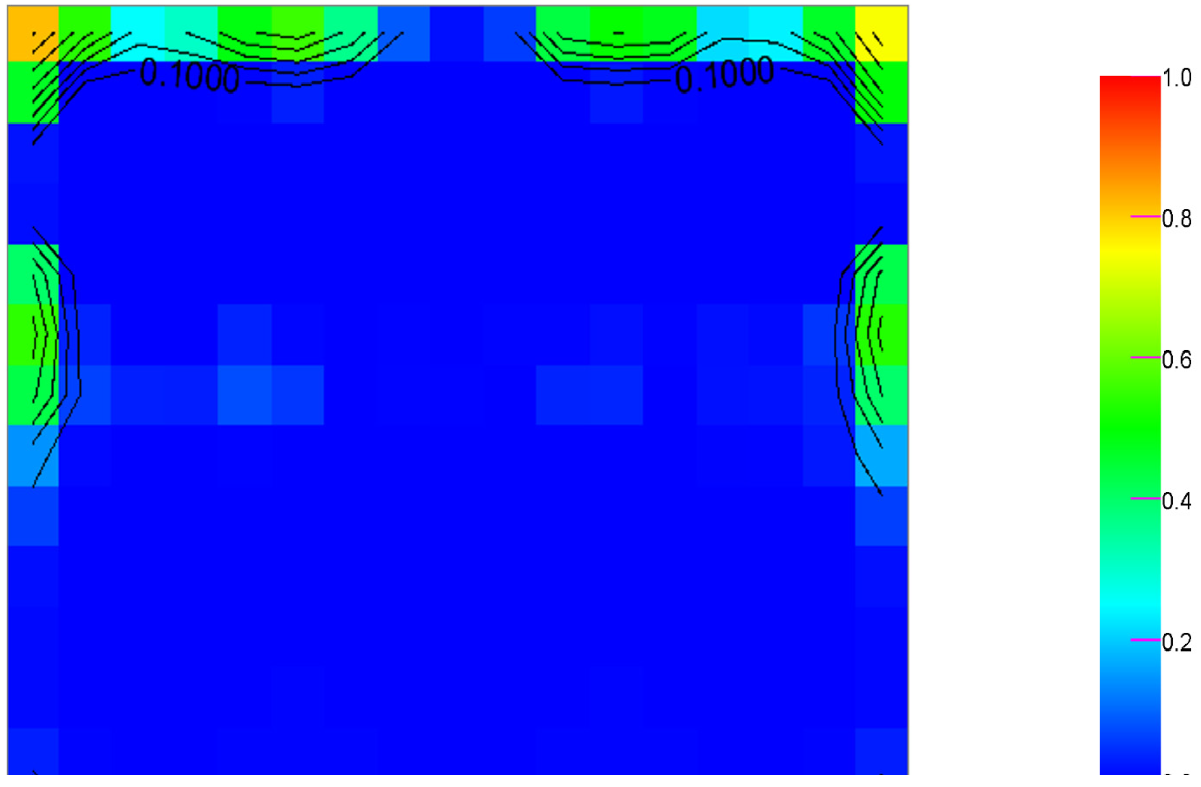
Automatic critical point determination can be easily implemented in software. Given a grid of work plane analysis points for a specified task area across which a particular minimum target illuminance is desired, software can determine the lowest dimming level that meets this goal under any daylight condition. Using such an analysis, the point that governs the setting of the electric lighting system for a particular hour is referred to as the “critical point” for that daylight condition. If the critical point location is determined for each hour of the year and the number of hours at which each point is the critical point is then tallied, the points that most frequently serve as the critical point can be identified. Results from such a study generally show that the critical point is located in one or more consistent locations [
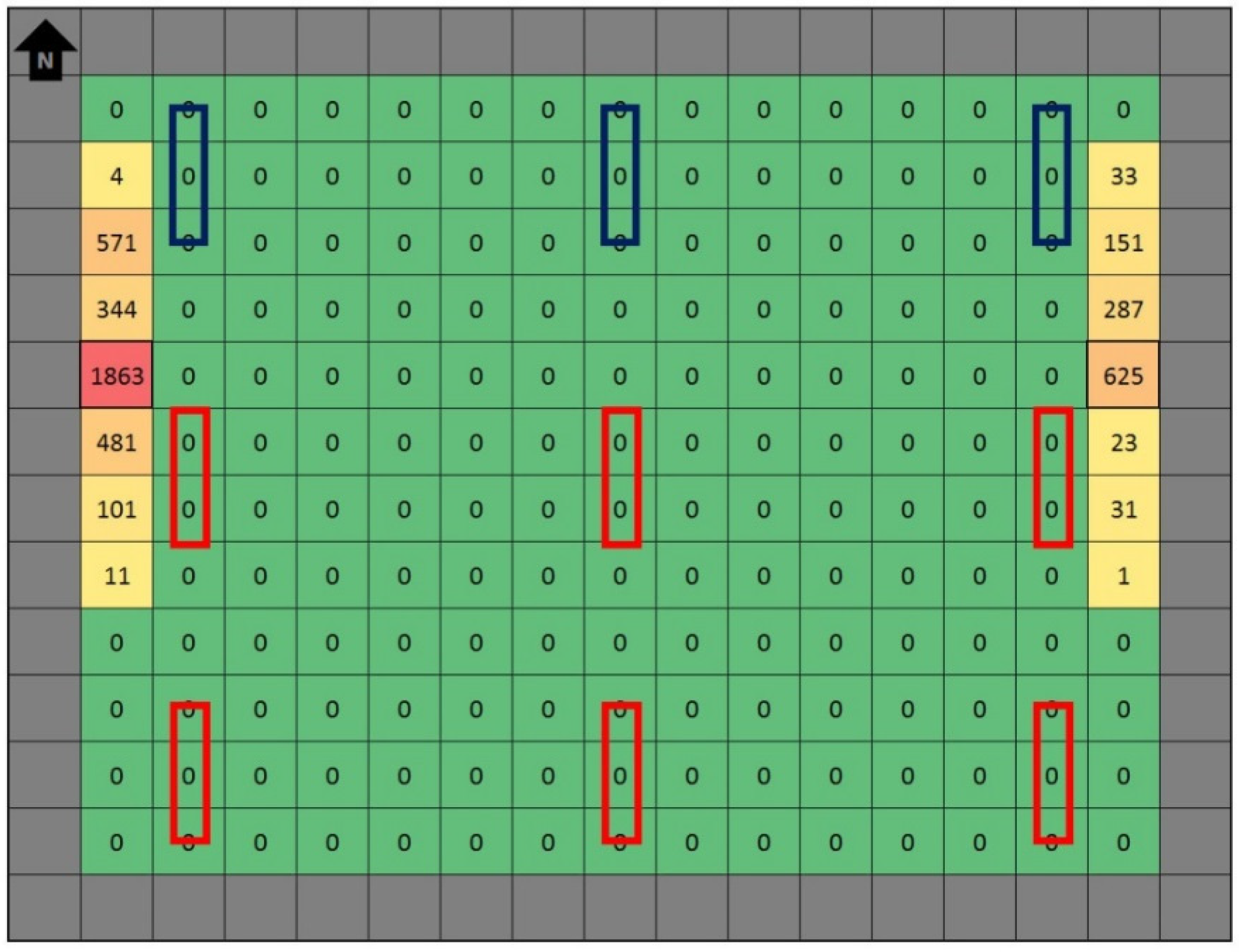
21] as shown in
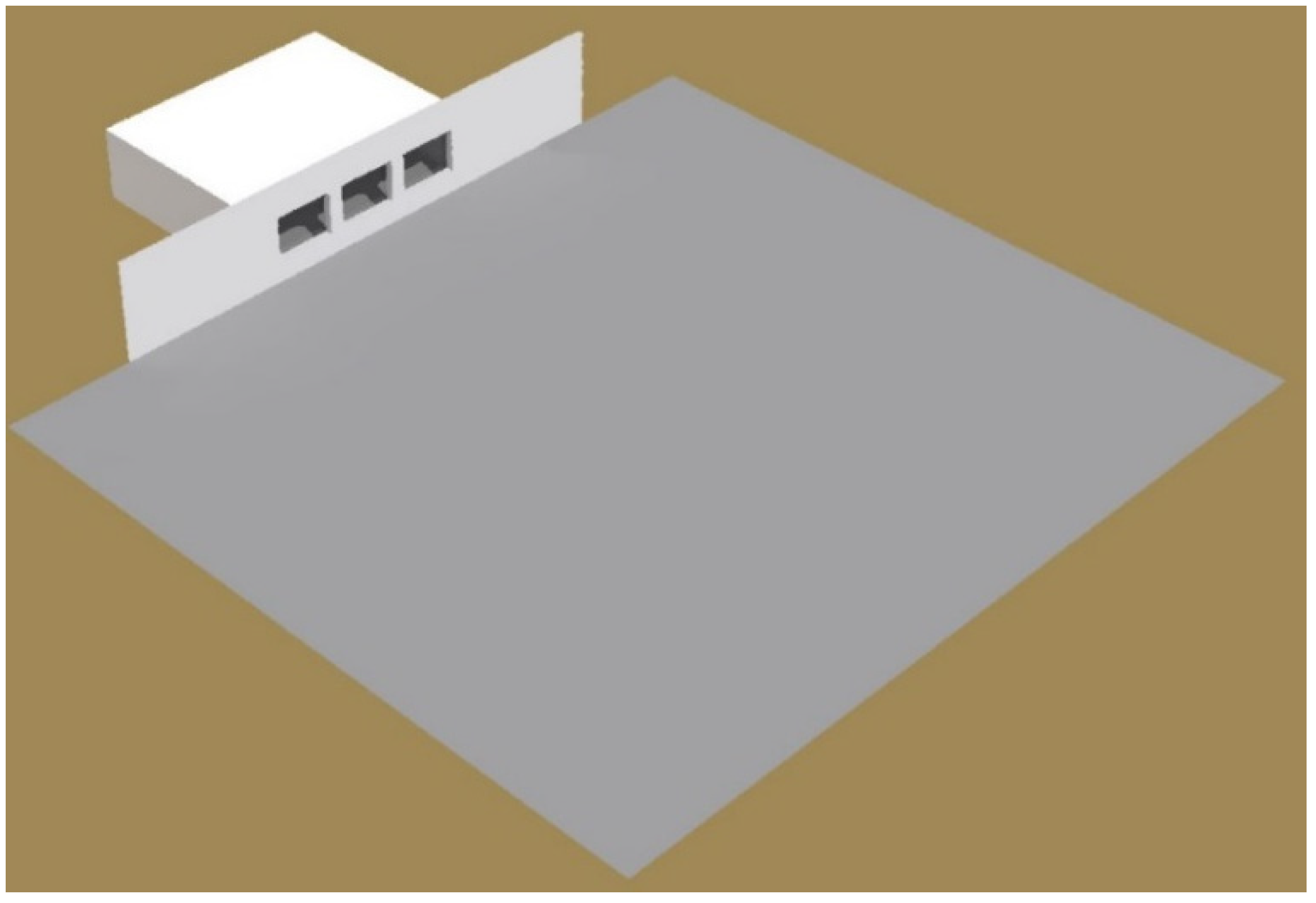
Figure 1, which considers a 12.1 m × 10 m × 3.6 m (34 ft × 28 ft × 10 ft) classroom model (illustrated in
Figure 2) that has the material properties described in
Table 1. The three windows are each 2.8 m wide × 2.1 m high. In this south-facing space, the most common locations for the critical point alternate between positions along the east and west walls depending on the time of day, since the sun’s position and the resulting sky brightness surrounding the sun will affect which side of the room is brighter. When calibrating a photocontrolled lighting system in a real space, the work plane point at which an illuminance meter is placed for the purpose of establishing an appropriate dimming level for the calibration time daylight condition should be one of these critical points.
Figure 1.
Plan view of a room showing a tally of the critical point locations across the year for a control zone that consists of two rows of luminaires with daylight entering through windows along the south wall. The top row of luminaires in this figure is not dimmed.
Figure 1.
Plan view of a room showing a tally of the critical point locations across the year for a control zone that consists of two rows of luminaires with daylight entering through windows along the south wall. The top row of luminaires in this figure is not dimmed.
Figure 2.
A 12.1 m × 10 m × 3.6 m classroom that is used for general modeling purposes throughout this paper. The classroom has three south-facing windows.
Figure 2.
A 12.1 m × 10 m × 3.6 m classroom that is used for general modeling purposes throughout this paper. The classroom has three south-facing windows.
In assessing the energy savings potential and proper control system operation, the use of two critical points can provide a reasonable assessment of an optimum control condition. Basing the energy savings on only a single point can overestimate these savings in situations where the critical point moves from one side of the room to another, which is quite common. Considering the critical point to be located along the centerline of the room is not recommended since it will overestimate the energy savings due to the higher daylight levels in this area compared to points closer to the walls. For best results, the application of at least two critical points is recommended. An analysis where the critical point is permitted to float across all points in a space is another option. In the case of the room shown in
Figure 1, 14 critical points would be applied and the target illuminance would be achieved at all points within the space at all hours of the year, with slightly higher energy consumption than would be obtained with fewer critical points.
Table 1.
Material properties for the daylighted classroom model.
Table 1.
Material properties for the daylighted classroom model.
| Surface | Reflectance (or Transmittance) |
|---|
| Ceiling | 0.8 |
| Walls | 0.6 |
| Floor | 0.3 |
| Façade | 0.4 |
| Ground | 0.2 |
| Windows | τ = 0.65 |
| Shade Fabric | τ = 0.12 diffuse, ρ =50% |
2.4.2. Qualifying Points for a Critical Point Analysis
It may be prudent to exclude certain work plane positions from the critical point analysis. Points that are outside the critical task area where the major visual work in a space is performed, such as points in a circulation area adjacent to a wall in a classroom, are generally unimportant and can be excluded. Other points that can be excluded include those that have almost no contribution from the controlled lighting zone. In this case, a threshold value for the control zone illuminance at a point can be applied to exclude points from consideration as the critical point when they are well outside the controlled lighting zone. For example, points might be excluded when the contribution from the controlled lighting zone falls below 10% or 20% of the target illuminance.
2.5. Photosensor Signals and Control Algorithms
Since the real-world performance of a photocontrolled lighting system is largely dictated by the signal received by the photosensor, and the conversion of this signal to an appropriate dimming level using the available algorithm, these system features must be assessed in an attempt to replicate real-world performance. Past studies have shown that sensors with a significant view of a window, or of a patch of direct sunlight, could result in overdimming of the electric lighting system [
22,
23,
24,
25]. Both photosensor directional sensitivity and position/aiming affect the signal reading. These effects can be studied using modeling software. Once the signals related to the electric lighting zones and the daylight are known, the software can test how well the algorithm can be configured to adequately dim the controlled lighting zone. If the photosensor is located within a space, dimming of the controlled lighting zone is likely to affect the magnitude of the photosensor signal and it is a closed-loop device. In applying the control algorithm, the equilibrium condition must then be determined for which the dimming level produces a combined photosensor signal from all sources that, when passed through the algorithm, calls for that same dimming level.
2.5.1. Photosensor Modeling
The hourly signal from the photosensor can be simulated using daylight coefficients or matrices that are linked to an array of sky patches and/or sun locations with Perez sky luminance data. The photosensor’s spatial sensitivity, which is not currently available from most manufacturers, dictates the magnitude of the signal for different daylight and shading conditions, and along with the photosensor position is an essential input to any analysis.
2.5.2. Applying a Control Algorithm
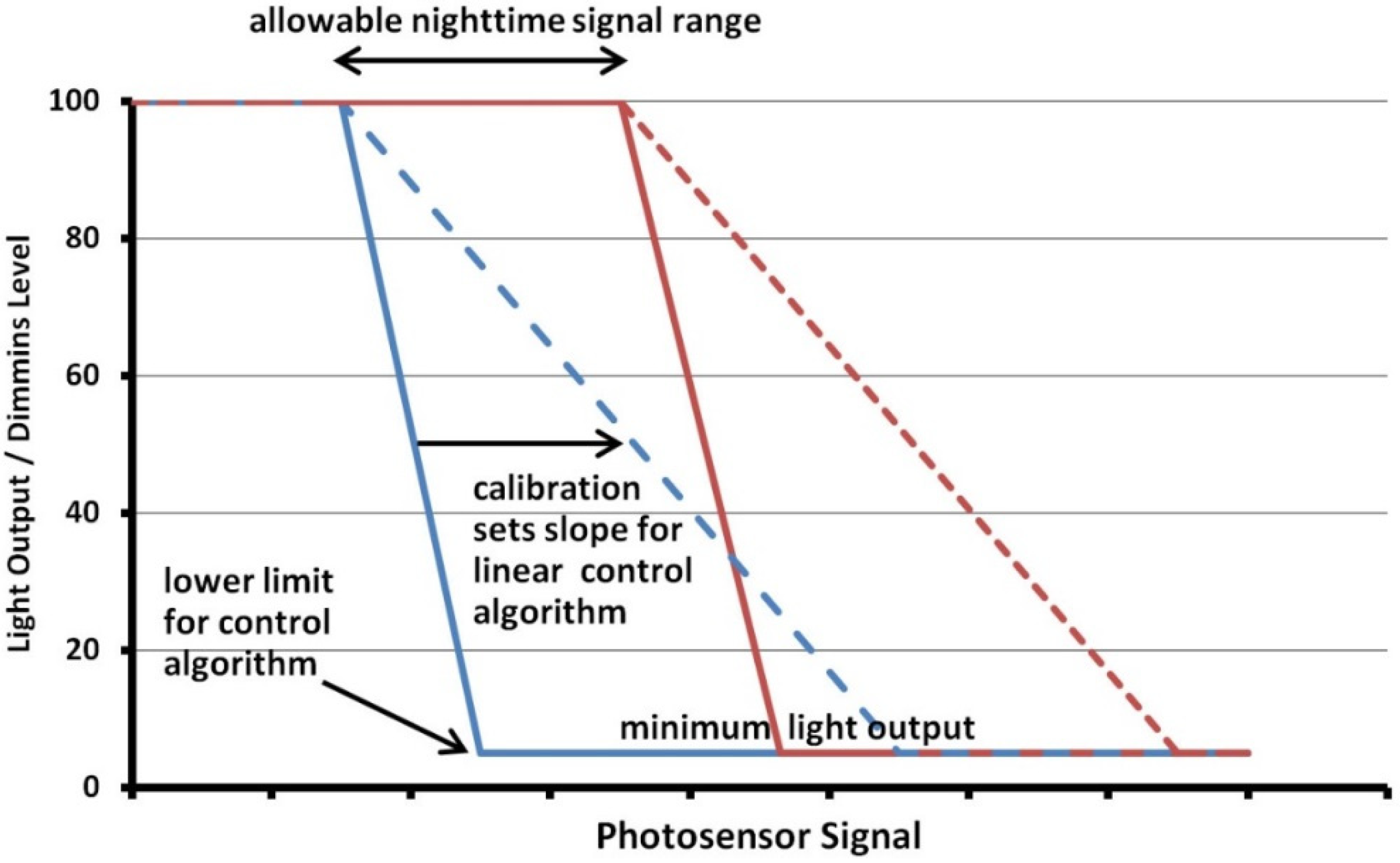
Once the photosensor signals are obtained, a calibration condition is then selected to establish the best setting for the photosensor system’s control algorithm. Control algorithms can include standard algorithms such as linear proportional control or closed-loop constant setpoint control (sometimes referred to as integral reset). Some manufacturers apply non-linear control algorithms, in which case the algorithms signal to dimming level relationships must be entered into the software for it to compute the best possible control algorithm settings. Previous measurements of control algorithms have uncovered a variety of non-standard algorithms [
26]. Investigations into the performance of these algorithms could identify those products that provide the most desirable control of the electric lighting system. At present, manufacturers do not generally provide photosensor algorithm information with which to conduct these studies, but as the use of these products becomes more widespread, and modeling such as discussed in this paper becomes commonplace in design practice, this information will be necessary.
Finally, keep in mind that the layout of the controlled lighting zone and the daylight distribution within a space will affect how a daylight-integrated lighting control system will perform. Connections to software that contains this information, such as Building Information Modeling (BIM) software that is used in the design process, as well as readily available performance data on complex fenestration systems (primarily shading devices), will provide additional input that improves the ability to quickly model real-world conditions and fine-tune these designs.
4. Conclusions
The analysis techniques and concepts displayed in this paper are intended to introduce the reader to a range of different approaches that can be used to assess and compare the performance of photocontrolled electric lighting systems, with the goal of delivering a more optimized design. With the implementation of these approaches, product selection, system layout, and design can be based on data from simulations that model the photosensor-based control system as it is expected to perform in the field. Characteristics that are modeled include the surrounding environment (interior and exterior), the daylight aperture conditions (including shading device operation), a photosensor’s directional response and control algorithm, and the layout of the electric lighting system and control zone.
With the future increase in the application of these systems that is certain to occur, tools that assist in the layout of these systems by assessing product performance in a manner that replicates how the system is expected to perform in a real installation are needed. Packaged software solutions, which minimize the time and effort required to perform these analyses, are likely to have the greatest market penetration and impact. The application of these tools will require lighting control system manufacturers to provide more detailed performance data on their products. This can easily be accomplished through the application of a standard format file, similar to that which is used for luminaires, except that it would include spatial sensitivity data, limits on the operating signal range, and a complete description of the algorithm that is used to convert a photosensor signal to a lighting control condition. This will provide designers with the ability to identify those products that provide the best overall performance for the space conditions being considered and fine-tune their designs. The net effect should be improved system performance, greater occupant acceptance, and higher levels of energy savings.
Acknowledgments
This material is based upon work supported by the Energy Efficient Buildings Hub (EEB Hub) and the Consortium for Building Energy Innovation, with support from the U.S. Department of Energy under Award number DE-EE000426.
Disclaimer
This report was prepared as an account of work sponsored by an agency of the United States Government. Neither the United States Government nor any agency thereof, nor any of their employees, makes any warranty, express or implied, or assumes any legal liability or responsibility for the accuracy, completeness, or usefulness of any information, apparatus, product, or process disclosed, or represents that its use would not infringe privately owned rights. Reference herein to any specific commercial product, process, or service by trade name, trademark, manufacturer, or otherwise does not necessarily constitute or imply its endorsement, recommendation, or favoring by the United States Government or any agency thereof. The views and opinions of authors expressed herein do not necessarily state or reflect those of the United States Government or any agency thereof.
Author Contributions
This paper is based on development work on software tools and performance studies of photocontrol systems that have been conducted over the past few years at Penn State University by Craig Casey, Ling Chen, and Sarith Subramaniam under the direction of Richard Mistrick. Richard Mistrick drafted the text, while the co-authors contributed figures, comments, and suggestions, and assisted in the development of software tools and analysis techniques that are discussed in this paper.
Conflicts of Interest
The authors have been involved in the development of the DAYSIMps software, which currently contains a large number of the features described in this paper (but not all). DAYSIMps is open-source software and is distributed for free.
References
- American Society of Heating, Refrigerating, and Air-Conditioning Engineers (ASHRAE). ANSI/ASHRAE/IES Standard 90.1-2013—Energy Standard for Buildings Except Low-Rise Residential Buildings; ASHRAE: Atlanta, GA, USA, 2013. [Google Scholar]
- American Society of Heating, Refrigerating, and Air-Conditioning Engineers (ASHRAE). ANSI/ASHRAE/IES Standard 189.1-2014—Standard for the Design of High-Performance Green Buildings except Low-Rise Residential Buildings; ASHRAE: Atlanta, GA, USA, 2014. [Google Scholar]
- California Energy Commission. 2013 Building Energy Efficiency Standards for Residential and Nonresidential Buildings; California Energy Commission: Sacramento, CA, USA, 2013. Available online: http://www.energy.ca.gov/2012publications/CEC-400-2012-004/CEC-400-2012-004-CMF-REV2.pdf (accessed on 30 January 2015).
- International Code Council (ICC). International Energy Conservation Code 2012; ICC: Washington, DC, USA, 2012. [Google Scholar]
- U.S. Green Building Council (USGBC). LEED Reference Guide for Building Design and Construction, LEED V4; USGBC: Washington, DC, USA, 2013.
- Heschong Mahone Group, Inc. Sidelighting Photocontrols Field Study, Final Report. 2005. Available online: https://www.sce.com/NR/rdonlyres/B460443C-7F82-4EFD-AEBF-F80E00FC5106/0/CS_0407_Sidelit_Photocontrols_Final.pdf (accessed on 30 January 2015).
- Architectural Energy Corporation. Sensor Placement and Optimization Tool. 2011. Available online: http://www.daylightinginnovations.com/spot-home (accessed on 30 January 2015).
- Daylighting Innovations. Sensor Placement and Optimization Tool. Available online: http://www.daylightinginnovations.com/spot-home (accessed on 30 January 2015).
- Mistrick, R.; Casey, C. Performance Modeling of Daylight Integrated Photosensorcontrolled Lighting Systems. In Proceedings of the 2011 Winter Simulation Conference, Phoenix, AZ, USA, 11–14 December 2011.
- The Pennsylvania State University. DAYSIM—Advanced Daylight Simulation Software, New DAYSIMps Tool. Available online: http://daysim.ning.com/page/download (accessed on 30 January 2015).
- Lawrence Berkeley National Laboratory. Radiance Reference. Available online: http://radsite.lbl.gov/radiance/framew.html (accessed on 30 January 2015).
- Larson, G.W.; Shakespeare, R.A. Rendering with Radiance—The Art and Science of Lighting Visualization; Morgan Kaufmann Publishers: San Francisco, CA, USA, 1998. [Google Scholar]
- Illuminating Engineering Society (IES). Approved Method: IES Spatial Daylight Autonomy (sDA) and Annual Sunlight Exposure (ASE); IES: New York, NY, USA, 2013. [Google Scholar]
- Ward, G.; Mistrick, R.; Lee, E.S.; McNeil, A.; Jonsson, J. Simulating the daylight performance of complex fenestration systems using bidirectional scattering distribution functions within radiance. Leukos 2011, 7, 241–261. [Google Scholar] [CrossRef]
- McNeil, A. The 5-Phase Method. Presented at the 12th International Radiance Workshop, Golden, CO, USA, 12–14 August 2013; Available online: http://www.radiance-online.org/community/workshops/2013-golden-co (accessed on 30 January 2015).
- Van den Wymelenberg, K. Patterns of occupant interaction with window blinds: A literature review. Energy Build. 2012, 51, 165–176. [Google Scholar] [CrossRef]
- Energy Plus—Input Output Reference; The Board of Trustees of the University of Illinois and the Regents of the University of California: Berkeley, CA, USA, 2014. Available online: http://apps1.eere.energy.gov/buildings/energyplus/pdfs/inputoutputreference.pdf (accessed on 30 January 2015).
- Illuminating Engineering Society (IES). ANSI/IES LM63-02—Standard File Format for Electronic Transfer of Photometric Data; IES: New York, NY, USA, 2008. [Google Scholar]
- Heart Consultants Ltd. EULUMDAT file format Specification. Available online: http://www.helios32.com/Eulumdat.htm (accessed on 30 January 2015).
- The Lighting Handbook: Reference & Application; DiLaura, D.; Houser, K.; Mistrick, R.; Steffy, G. (Eds.) IES: New York, NY, USA, 2011.
- Casey, C.; Mistrick, R. Determining the Critical Point for Design, Analysis, and Commissioning of a Photocontrolled Dimming System. In Proceedings of the 2012 IES Annual Conference, Minneapolis, MN, USA, 11–13 November 2012.
- Mistrick, R.; Chen, C.-H.; Bierman, A.; Felts, D. A comparison of photosensor-controlled electronic dimming systems in a small office. J. Illum. Eng. Soc. 2000, 29, 66–80. [Google Scholar] [CrossRef]
- Shashikala, R.; Mistrick, R. A study of photosensor configuration and performance in a daylighted classroom space. J. Illum. Eng. Soc. 2003, 32, 3–20. [Google Scholar]
- Mistrick, R.; Sarkar, A. A study of daylight-responsive photosensor control in five daylighted classrooms. LEUKOS 2005, 1, 51–74. [Google Scholar]
- Kim, S.Y.; Song, K.D. Determining photosensor conditions of a daylight dimming control system using different double-skin envelope configurations. Indoor Built Environ. 2007, 16, 411–425. [Google Scholar] [CrossRef]
- Bierman, A. Photosensors; NLPIP Specifier Reports. Lighting Research Center: Troy, NY, USA, 2007. Available online: http://www.lrc.rpi.edu/nlpip/publicationDetails.asp?id=916&type=1 (accessed on 30 January 2015).
- Chen, L. Sensor Performance of Advanced Photocontrol Systems. Master Thesis; The Pennsylvania State University: University Park, PA, USA, 2013. Available online: https://etda.libraries.psu.edu/paper/19943/ (accessed on 30 January 2015).
- Subramaniam, S.; Chen, L.; Mistrick, R. Annual Performance Metrics for Photosensor-Controlled Daylight-Responsive Lighting Control Systems. In Proceedings of the 2013 IES Annual Conference, Huntington Beach, CA, USA, 27–29 October 2013.
© 2015 by the authors; licensee MDPI, Basel, Switzerland. This article is an open access article distributed under the terms and conditions of the Creative Commons Attribution license (http://creativecommons.org/licenses/by/4.0/).


