What Can We Learn from the Household Electricity Survey?

Abstract

The reasons for high carbon emissions from domestic buildings are complex, and have both social and technical dimensions. At the same time, it is costly and very time-consuming to gather reliable data on energy use in the home. The authors had early access to data from the Household Electricity Survey—the most detailed survey of electricity consumption in UK homes ever undertaken—which monitored 250 homes. The data enabled the authors to investigate a series of socio-technical questions drawn up by the UK Government: Why do some households use far more energy than average, whereas others use much less? What potential is there for shifting “peak load” so that electricity demand is more even through the day? Why is base load electricity use so high? The answers were seldom definitive, but statistical tests found significant correlations between high electricity use and social grade, large household size, unemployment and middle age; and between low electricity use and single-person households, small dwellings, and retirement. This paper draws out key findings from the work, and examines how these insights affect our broader understanding of carbon emissions from the built environment.

1. Introduction

Internationally there is a perennial problem in collating reliable data about energy use. This makes it much harder to assess progress towards energy efficiency objectives and to introduce effective policies [1]. The United Kingdom has made considerable progress in producing detailed, systematic statistics covering different sectors of the economy. However, even in countries which regularly gather detailed data, there are limits to the understanding that can be gleaned from national statistics [2]. For energy use in the building sector, bottom-up surveys are an important complement to aggregate figures based on energy sales. This is particularly true when it comes to uses that are highly dependent on behaviour, such as for household appliances.

Within the UK, homes account for more than a quarter of the national energy use and carbon dioxide emissions. More energy is consumed in housing than either the road transport or industry sectors. Moreover, residential energy use has been rising by an average of 0.4% a year since 1970 [3]. Consequently, housing represents a significant opportunity for emissions reductions if the UK is to meet its targets for 2050. In 2008, the UK introduced legally binding national targets to cut greenhouse gas emissions by 80% by 2050, compared with 1990 levels [4]. As part of meeting this requirement, the Government and its Department of Energy and Climate Change (DECC) have identified a need to reduce electricity consumption in the home [5].

Electricity, as a proportion of total household energy use, varies from year to year, but in 2012 it accounted for 22%, or 109 TW·h [3]. In the UK, the carbon intensity of grid electricity is high compared to natural gas, which makes up almost two-thirds of residential energy use [6]. This is due to losses in electricity generation and the primary fuels, and means that, despite making up less than a quarter of the energy consumed, electricity accounts for 48% of household emissions; almost 60 million tonnes of CO₂ annually. Electricity consumption in the home has grown by two-fifths over the past 44 years [3], and the Office of Gas and Electricity Markets (Ofgem), has expressed concerns about maintaining sufficient electricity generating capacity, and ensuring the UK can continue to meet its peak electricity demand [7].

In 2010, DECC, in conjunction with the Department for Environment, Food and Rural Affairs (DEFRA) and the Energy Saving Trust, commissioned the Household Electricity Survey (HES) to improve the understanding of residential energy performance. The following section provides an overview of the HES. Further details are available elsewhere [8,9,10].

1.1. The Household Electricity Survey

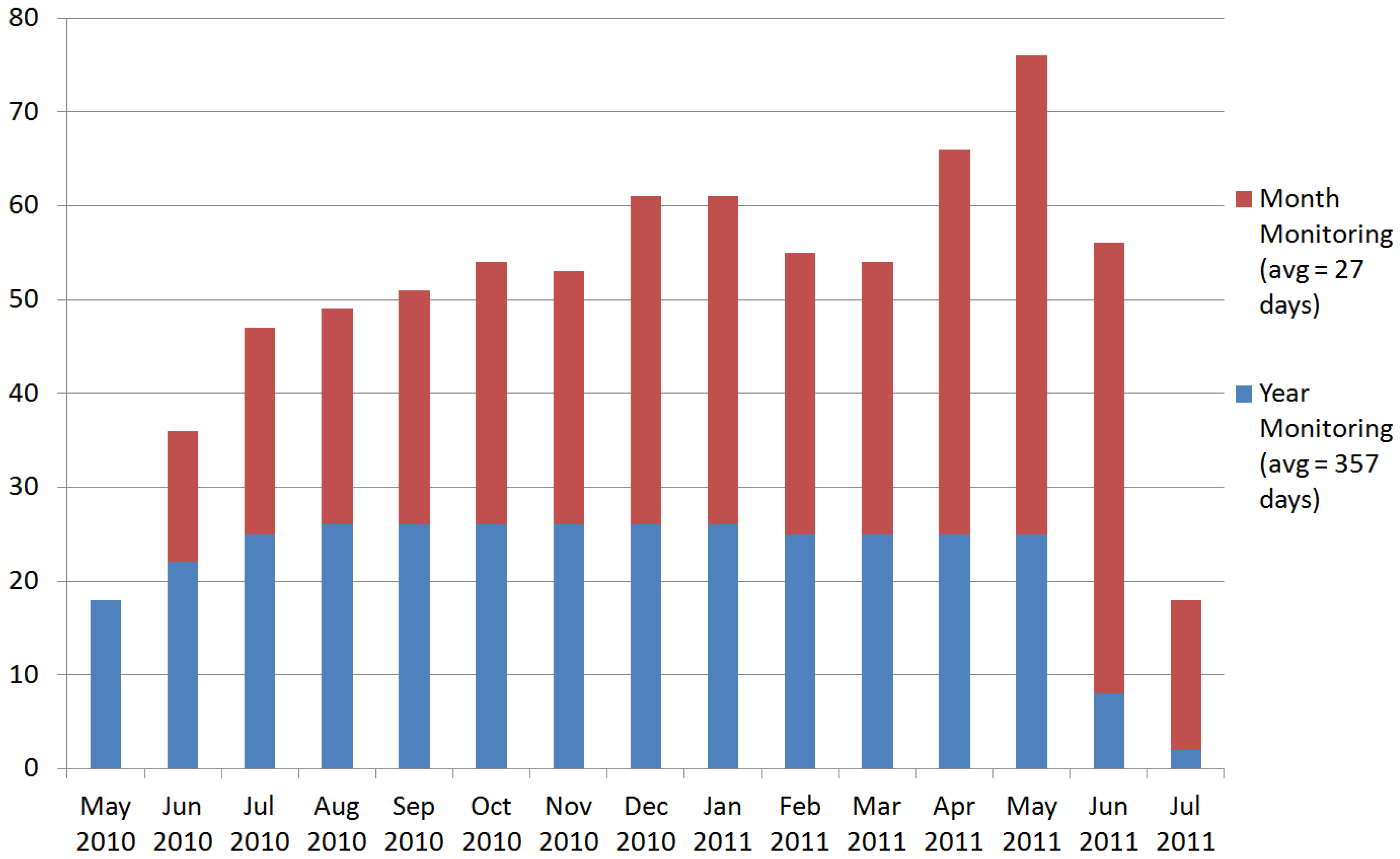
Electricity use was metered in 250 owner-occupier dwellings across England during 2010 and 2011. Of these, 26 were monitored for a full year, and the remainder for one month, each on a rolling basis throughout the timeframe of the survey. For each home, metering was attached centrally to the distribution boards, and to key individual appliances. These recorded electricity use at 10 min intervals for a year or 2 min intervals for a month. Most of the analysis was performed at a resolution of ten minutes, the two minute records having been combined to make longer intervals. However, the 2 min data was used where the finer resolution was appropriate. The mean annual electricity consumption for the HES sample was 4093 kW·h, compared with 4154 kW·h for the UK in 2011 [11].

The number of appliances monitored per household varied between 13 and 85, and covered wet and cold appliances, as well as Information and Communication Technology (ICT) equipment, some consumer electronics and lighting. For homes that were monitored for a single month only, Meter Point Administration Number (MPAN) data was also collected, which provided total household electricity use for the year 2010. Although similar studies have been conducted elsewhere (e.g., [12]), the scale and resolution of the monitoring makes the HES the most detailed electricity use survey ever undertaken in the UK. Figure 1 below shows the breakdown of monitoring, split between the monthly and yearly houses. The precise period of monitoring varied from house to house, and did not always line up with the calendar. Therefore, the average monitoring period is also shown on the chart.

Figure 1. Number of homes monitored, month by month.

Figure 1. Number of homes monitored, month by month.

For each of the participating households, a survey was carried out to gather information on the electrical appliances and lighting within the building. Information collected included key variables such as model and energy efficiency ratings for white appliances, and lamp type and rated power for lighting. Finally, a questionnaire was completed by the occupants covering the residents’ working and social status, and their attitudes to energy use and climate change. This questionnaire was similar to the “tracker” surveys carried out each year by DEFRA [13]. It also covered the measures the households take to reduce electricity consumption. For example, 77% of the HES households claimed to fill the kettle only as much as necessary “quite often or more”, and 89% washed their clothes no warmer than 40 °C.

The dwellings included in the study cover much of England, and were selected to be broadly representative of the UK in terms of both physical and social factors, such as occupant social grade and employment status, household size and property age [8]. However, the HES sample differs notably from the national housing stock in three important respects. Firstly tenure (social and rented housing, which make up roughly 35% of the UK total [14], were excluded) and secondly household beliefs (the HES participants were found to be more energy-conscious than the UK average). Only nine of the households have electricity as the primary source of space heating, although 28% of the overall sample did include some form of secondary electric heating. Table 1 summarises the dwellings monitored.

Table 1. Characteristics of households in the Household Electricity Survey (HES) sample.

Data	Reported values	Month monitoring	Year monitoring
No. of households	–	224	26
No. of occupants	Mean	2.7	2.4
Dwelling size (m2)	Mean	96	103
No. of appliances	Mean	45	40
Social grade (%) *	A–B	34	19
–	C1–C2	52	69
–	D–E	13	12

* Social grade was unknown for one monthly household.

Table 1. Characteristics of households in the Household Electricity Survey (HES) sample.

Data	Reported values	Month monitoring	Year monitoring
No. of households	–	224	26
No. of occupants	Mean	2.7	2.4
Dwelling size (m2)	Mean	96	103
No. of appliances	Mean	45	40
Social grade (%) *	A–B	34	19
–	C1–C2	52	69
–	D–E	13	12

* Social grade was unknown for one monthly household.

1.2. Aims of This Paper

The HES presents a unique opportunity to examine current electricity use in UK homes. This article endeavours to use the data to improve the understanding of the relationship between behaviour, household social factors, and energy performance. More specifically, it builds upon prior work carried out by the authors [10], to produce new conclusions in two key research areas:

• How does electricity demand vary in a dwelling over time? This analysis focuses on two important aspects of energy profiles: the base load, and the peak load.
• How does electricity use vary between dwellings? This analysis examines the relationship between energy consumption, and different house, and household factors.

2. Domestic Electricity Use

Although the HES represents the most detailed residential electricity monitoring project undertaken in the UK at the time of writing, there have been smaller, similar studies that have explored the drivers of domestic energy use.

In the late 1990s, a study into the electricity demand in 30 UK homes found that occupancy and income were the main variables driving both total electricity use and daily demand profiles [15]. More recent studies have also found correlations between household income and electricity consumption, and examined the interrelationships between income and other variables. A study carried out in 2008 of data aggregated to small geographic areas determined that income is a key factor affecting residential energy use, but that a number of other variables were also critical, including the type of dwelling, tenure, and household size (i.e., the number of occupants) [16]. An examination of the National Energy Efficiency Data-framework (NEED), a large database of annual energy consumption in UK buildings, found that while electricity use varies with dwelling tenure, the underlying driver was likely to be household income [17]. Other variables found to correlate non-linearly to differences in electricity use included household and dwelling sizes. The analysis of NEED also observed different performance in homes of different ages, with mean electricity use in pre-1919 homes 10% higher than the overall stock. However, this relationship was less clear, and posited to be due to the changing trends in built form and fabric over time, as well as the uncertain nature of refurbishments. Analysis of household tenure was also covered in a study of 27 homes in Northern Ireland, which found far higher annual electricity use in owner-occupied homes than rented ones [18]. More specifically examining the relative impact of income and other factors, a multi-variate regression analysis of the electricity consumption in homes in Portugal found that, while income is a key driver, the impact of this variable is reduced once related factors including house type, size and occupancy are taken into account [19]. However, studies have noted large differences in energy demand across Europe [20] suggesting that the results cannot necessarily be assumed to be valid for the UK.

In addition to the differences in average annual electricity use, the complexity of occupant behaviour has been examined in many of the studies mentioned above. Most reference large variations in annual energy use between ostensibly similar dwellings, as well as differences in the daily demand profiles. It has been noted that behaviour in individual households varies from day to day and that coincidences of appliance use, particularly those with electric heating elements, are a key factor in determining the peak demand [15]. Unsurprisingly, the factors that impact on household electricity demand profiles have been found to overlap with those of annual consumption, with the time and magnitude of peak demand found to vary with income, dwelling size and household size [18].

At the scale of individual domestic appliances, differences in typical user behaviour have been observed between households. For instance, a recent study found higher mean daily hours of television use in local authority and social housing, compared with owner-occupied homes [21]. Elsewhere, a study of 72 homes found that, while the energy consumption for different appliances typically rises with the dwelling’s total electricity consumption, the correlation varies with appliance type [22]. The difficulty of considering these factors in energy modelling was noted in a recent major review, which highlighted the need for domestic models to better account for the range of appliance electricity use [23]: SAP and BREDEM, the well established building regulations models adapted for a number UK building stock models (e.g., [24,25]) estimate appliance electricity consumption based solely on occupancy and floor area.

3. Data Processing

The raw HES dataset consists of electrical energy readings, for individual appliances and on the distribution board circuits, recorded for between a month and a year for 250 homes. Consequently, prior to carrying out any analysis, significant data processing was required. This is outlined below:

a)

Unknown Energy Use: The HES incorporates considerable appliance-scale monitoring. However, comparison between the electricity profile data and the household appliance surveys revealed that not all appliances were individually monitored in every household. For example one household owned six televisions, of which only three were monitored. Where the distribution circuit-level monitoring showed electricity use that could not be assigned to a specific appliance, this was recorded as “unknown”. On average, across the HES sample, unknown uses account for 20% of the household total electricity consumption.

b)

Incomplete Readings: In some instances, readings were missing for parts of the day, typically at the start and end of the dwelling’s monitoring period. Partial day records were removed. One or two days were removed from five households and 14 days (out of 42) were removed from one household. There were no instances where an appliance’s data was completely lost, due to missing readings.

c)

Incorrect or Misclassified Readings: In a few cases, the monitored electricity profiles for individual appliances were significantly different to what would be expected for the appliance type. Where this occurred, the data was amended if possible. Some appliances were reclassified based on the household appliance survey data or the characteristics of the profile–for example several electric cookers that never used more than a few Watts were in fact extractor fans for gas cookers. Sometimes, a profile classified as a single appliance was in fact a number of appliances on the same socket. For example, one classified as a light shared a socket with a cordless phone and radio. Finally, unreasonable spikes in the profiles (such as a DVD player briefly using more than 2 kW) were removed and the profile data smoothed. The data from 90 appliances were reclassified.

d)

Duplicate Readings: Occasionally, profiles in the HES were duplicated, or one profile included another. This was particularly common with audiovisual appliances, presumably because of the use of daisy-chained power blocks. For example, a multi-way extension cable feeding a TV, set top box and DVD player, might be monitored as a whole at the wall, but the DVD player might also be monitored separately. Where duplicate readings were found, these were extracted. In all, 22 appliances data records were found to be either duplicates or incorporated in another profile.

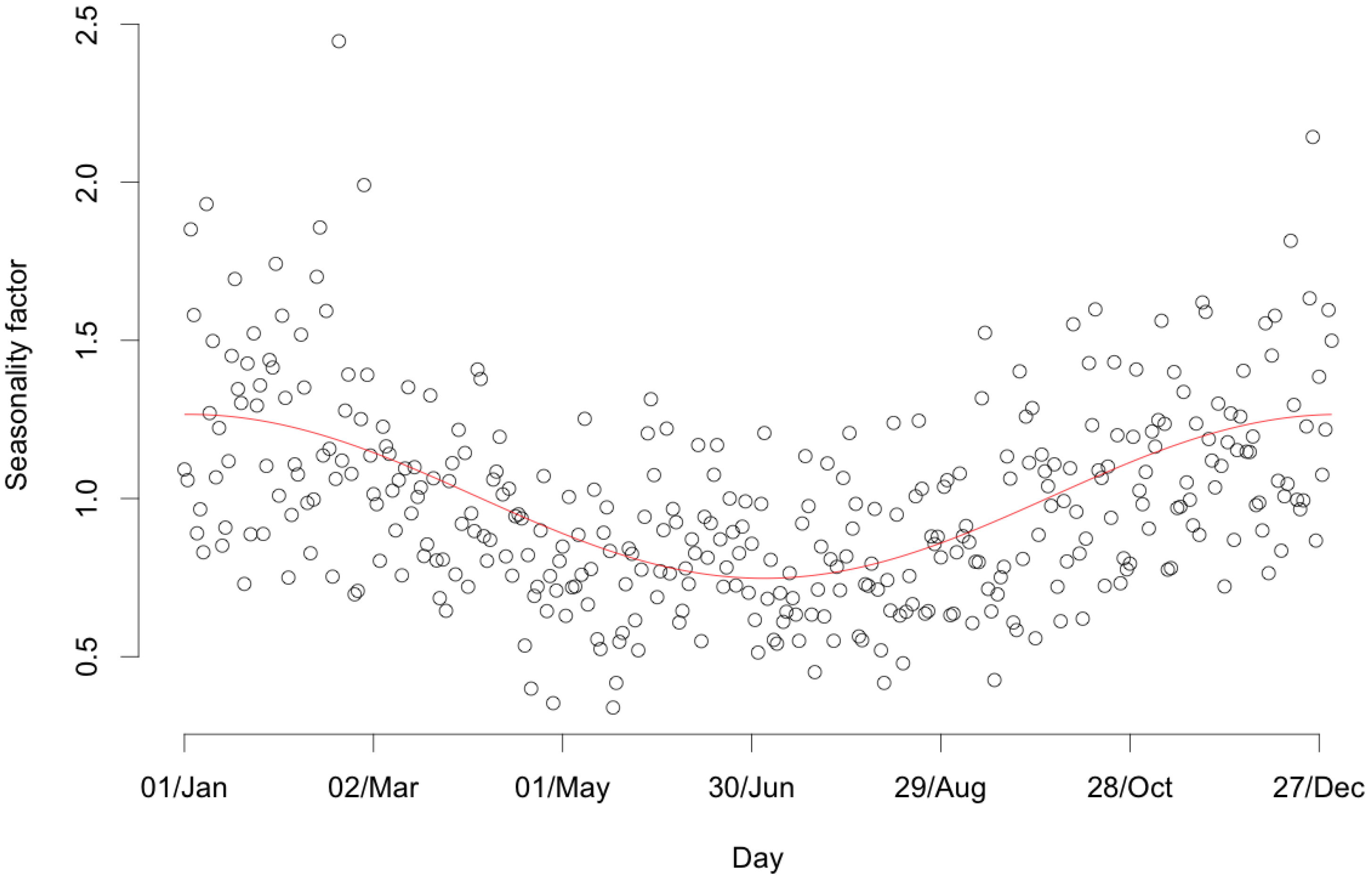
This study includes analysis of annual electricity use as well as the daily profiles of electrical demand. Therefore, in addition to the processing outlined above, it was necessary to scale up the results for the households monitored for only one month. Seasonal adjustment factors were used to account for variations in use through the year, caused by changes in occupant behaviour as well as the weather (see Figure 2).

Figure 2. Seasonal adjustment factor used for annualising washing energy data.

Figure 2. Seasonal adjustment factor used for annualising washing energy data.

For example, lighting is typically more heavily used in winter, when the evenings are dark and the daytimes not particularly bright, whereas refrigerators and freezers usually need more energy in the summer because the ambient temperature is higher. Washing energy use is often similarly seasonal, particularly for tumble dryers, since many households use a washing line for drying clothes when weather permits. Seasonal adjustment factors were generated for each appliance group by assigning best-fit sine or cosine curves to the data from the 26 households monitored for an entire year. Figure 2 presents the seasonal curve (in red) generated from the normalised raw monthly readings for each home monitored for a year (black circles) for washing appliances.

The seasonal adjustment process adds a level of uncertainty to any analysis, compared with examining the raw monitored data. Therefore, where possible, the unadjusted data has been used in the analysis presented here. The energy use profile analyses use the unadjusted data, while the sections examining annual consumption use the seasonally adjusted data.

Following the data processing, household electricity consumption was grouped by appliance type. Eleven categories were used, as shown in Table 2, along with the average annual electricity use for each. The figures presented are the mean for the entire HES sample. For example, homes with solely gas-based water heating have been included in the calculation as 0 kW·h/year, and homes with back-up immersion heaters may have very low annual electricity consumption.

Table 2. Summary of the eleven categories of electricity use. ICT: Information and Communication Technology; AV: Audiovisual Appliances.

Category	Appliances	Mean annual energy
Cold appliances	Fridges, freezers and fridge freezers.	566 kW·h (13.8%)
Cooking	Electric hobs and ovens, kettles, microwaves, toasters and other small cooking appliances (excluding gas cooking).	448 kW·h (10.9%)
Lighting	Internal and external lights, on lighting circuits or lamps plugged into sockets.	483 kW·h (11.8%)
Audiovisual	TVs, games consoles, set top boxes, hi-fi systems, radios and other AV appliances.	537 kW·h (13.1%)
ICT	Computers, monitors, printers, scanners and networking equipment.	207 kW·h (5.1%)
Washing appliances	Washing machines, washer-dryers, tumble dryers and dishwashers.	437 kW·h (10.7%)
Showers	Electric showers.	112 kW·h (2.7%)
Water heating	Immersion heaters (excluding gas water heating).	85 kW·h (2.1%)
Space heating	Electric fires and other space heating appliances (excluding gas space heating).	227 kW·h (5.5%)
Other	Other appliances not in the above categories, including hair dryers, massage beds, aquariums and pond pumps.	173 kW·h (4.2%)
Unknown	Electricity use recorded on electrical socket circuits but not recorded at the appliance level. We do not know what this energy was used for.	819 kW·h (20.0%)

Table 2. Summary of the eleven categories of electricity use. ICT: Information and Communication Technology; AV: Audiovisual Appliances.

Category	Appliances	Mean annual energy
Cold appliances	Fridges, freezers and fridge freezers.	566 kW·h (13.8%)
Cooking	Electric hobs and ovens, kettles, microwaves, toasters and other small cooking appliances (excluding gas cooking).	448 kW·h (10.9%)
Lighting	Internal and external lights, on lighting circuits or lamps plugged into sockets.	483 kW·h (11.8%)
Audiovisual	TVs, games consoles, set top boxes, hi-fi systems, radios and other AV appliances.	537 kW·h (13.1%)
ICT	Computers, monitors, printers, scanners and networking equipment.	207 kW·h (5.1%)
Washing appliances	Washing machines, washer-dryers, tumble dryers and dishwashers.	437 kW·h (10.7%)
Showers	Electric showers.	112 kW·h (2.7%)
Water heating	Immersion heaters (excluding gas water heating).	85 kW·h (2.1%)
Space heating	Electric fires and other space heating appliances (excluding gas space heating).	227 kW·h (5.5%)
Other	Other appliances not in the above categories, including hair dryers, massage beds, aquariums and pond pumps.	173 kW·h (4.2%)
Unknown	Electricity use recorded on electrical socket circuits but not recorded at the appliance level. We do not know what this energy was used for.	819 kW·h (20.0%)

4. Analysis

4.1. How Does Electricity Demand Vary Over Time?

The graphs in Figure 3 present the mean daily electrical power profile for all of the households in the study, across the whole year. The profiles for working days and holidays (defined here as weekends and any bank holidays) are shown separately, to demonstrate the variation in behaviour between different days. The curves have been obtained by averaging the days for each household and then across the sample. The averaging process has dampened the daily fluctuations in energy use. However, the dampening effect is less for the holidays as there are fewer data points.

Figure 3. Mean electricity demand profile for the 250 HES households on (a) working days and (b) holidays.

Figure 3. Mean electricity demand profile for the 250 HES households on (a) working days and (b) holidays.

The expected night-time base load, small morning peak, and larger evening peak can be clearly seen. Comparison between the working days and holidays graphs shows that on holidays the morning peak builds more slowly and the evening peak starts slightly earlier. Visual inspection of the graphs suggests that there is a fairly constant cold appliance electrical load throughout the day, and this forms a large proportion of the total during the night. It also shows rising audiovisual, lighting and cooking uses contributing to the peak demand in the evening. In order to better understand the processes behind the profiles, examine the variations between households, and identify potential areas for energy or emissions savings, the base and peak loads were explored in more detail.

The sections that follow examine the electricity use base load and the evening peak in turn. For this work, the analysis was carried out on the overall average daily electricity use profile, without splitting between working days and holidays. As can be seen in the graphs above, the magnitude and timings of these are similar between the two day types.

4.1.1. The Characteristics of Electricity Base Loads

The electrical “base load” is the level that demand will rarely fall below. The precise definition tends to vary between studies, in terms of duration and whether the time should be continuous or not. Two recent methods to approximate residential base load have been “the power demand [...] exceeded for 90% of the monitoring period” [21] and “a single value [...] every two days that corresponded to that half-hour when the least electricity was consumed” [18].

For this study, for each household the mean electricity demand was calculated for each hour of the day from the monitored data. The minimum hourly value was then identified as the base load. As illustrated in the previous graphs, this typically occurred during the night. However, for 8% of the homes, the base load was during the day. This behaviour could reflect specific lifestyles (e.g., nightshift workers), but unfortunately, the level of occupancy information was not sufficient to determine the precise cause.

Past studies have suggested that residential electrical base load varies seasonally, albeit to a lesser extent than heating [18]. To examine this in more detail, the base load was calculated separately for energy data collected from October to March (130 households) and that collected from April to September (160 households). The characteristics of each set of households were similar, as shown in Table 3, although there were more single person households in the April to September group.

Table 3. Characteristics of households monitored in April–September and October–March.

Data	Reported value	April–September	October–March
No. of households	–	160	130
No. of occupants	Mean	2.4	2.6
Dwelling size (m2)	Mean	101	101
No. of appliances	Mean	41	41
Household types (%)	Single person	30	24
	Pensioners	23	28
	With children	31	32
	Working full-time	33	31
Social grade (%)	A–B	31	32
	C1–C2	55	53
	D–E	13	15
	Unknown	1	0

Table 3. Characteristics of households monitored in April–September and October–March.

Data	Reported value	April–September	October–March
No. of households	–	160	130
No. of occupants	Mean	2.4	2.6
Dwelling size (m2)	Mean	101	101
No. of appliances	Mean	41	41
Household types (%)	Single person	30	24
	Pensioners	23	28
	With children	31	32
	Working full-time	33	31
Social grade (%)	A–B	31	32
	C1–C2	55	53
	D–E	13	15
	Unknown	1	0

Figure 4 shows the mean base load power consumption across the sample for these two periods. The base load has been split by energy use, in order to examine the impact of different appliances.

Figure 4. Mean base load electricity demand per household, classified by appliance group.

Figure 4. Mean base load electricity demand per household, classified by appliance group.

Across the sample, the mean total base load is 175 W in April-September and 207 W in October–March. As expected, the analysis revealed considerable variation between individual households, with inter-quartile ranges of 83–220 W in summer, 99–217 W in winter. The largest proportion of known base load use is for cold appliances. This accounts for 41% of the known electricity demand, and 30% of the total. Of the remaining uses, “unknown” accounts for 50 W, while audiovisual equipment accounts for 23 W, approximately a third as much as cold appliances.

The seasonal variation in base loads for each appliance group was examined using Student’s t-tests, carried out using a p-value threshold of 0.05 to determine statistical significance. This analysis revealed that, for the sample buildings, cold appliances do exhibit a statistically significantly different base load between summer and winter (p = 0.04), as does space heating (mostly night-time storage heaters, p = 0.04). Both these trends are likely due to the reduced ambient temperature between summer and winter, which impacts on heat loss and the refrigerator performance. The other seasonal differences were not significant, including the unknown portion of the electricity use. A proportion of the electrical base load may be unavoidable for practical reasons (e.g., storage heaters charging at night, or refrigerator compressors firing periodically) or behavioural reasons (e.g., lighting left on at night for security). However, households vary in the number of appliances left on, so significant differences in base load across the sample may point to opportunities for energy saving through behaviour change, or efficiency improvements. To examine this issue, the distribution in base loads was analysed to identify any large variations. Figure 5 shows the distribution across the sample for the key appliance categories, showing the different patterns observed.

For most uses, such as cold appliances, almost all households were found to have considerable base loads. However, as the graphs above reveal, for three of the appliance categories, energy use in a small number of households is responsible for a substantial proportion of that appliance type’s contribution to the total base load. For example, while most households’ ICT base load was low, a few households were found to leave computers on at full power overnight. Table 4 shows the proportion of “high use” households in the sample, using cutoffs selected to account for roughly two-thirds of the total base load for each appliance group. It shows that 60% of the total ICT base load can be attributed to only 12% of the households. While there may be instances where this high base load is intentional and unavoidable, properly targeted interventions aimed at the high consuming households for these uses could have a large impact on total residential base load power demand, and be more efficient than blanket interventions. The results suggest that lighting and audiovisual and ICT appliances are the obvious candidates for these types of interventions.

Figure 5. Base load electricity consumption from April to September for specific appliance categories. Each blue line represents one household.

Figure 5. Base load electricity consumption from April to September for specific appliance categories. Each blue line represents one household.

Table 4. Appliance categories with small numbers of “high use” households.

Appliance category	Base load cut off (W)	Households above cut off (%)	Appliance base load from “high use” households (%)
Lighting	20	17	71
Audiovisual	30	22	59
ICT	20	12	60

Table 4. Appliance categories with small numbers of “high use” households.

Appliance category	Base load cut off (W)	Households above cut off (%)	Appliance base load from “high use” households (%)
Lighting	20	17	71
Audiovisual	30	22	59
ICT	20	12	60

4.1.2. Peak Electricity Demand

Peak load is a critical factor for electricity infrastructure. For the UK, it typically occurs around 6 p.m. to 7 p.m., and-with the relatively low level of domestic air conditioning-is highest during the winter [26]. It represents the most difficult time for energy companies and network operators to meet demand, and this brings higher costs and carbon emissions. Throughout the year, residential demand varies as a fraction of the UK’s overall peak, from 43% on a typical day to as much as 66% on the coldest days [27]. Consequently, reducing the demand peaks in the domestic building stock would be beneficial. In the HES, 115 households were monitored between 21 October and 21 February, and these were analysed to examine the potential for reducing the peak electricity demand in winter. Figure 6 shows the resulting mean total energy use profile in winter. This reveals a peak electricity demand of 970 W per household, just after 6 p.m. Typically, the peak is when householders have turned lights on and are preparing the evening meal or doing other activities.

Figure 6. Mean electricity demand profile for winter on (a) working days and (b) holidays.

Figure 6. Mean electricity demand profile for winter on (a) working days and (b) holidays.

One means of reducing the peak demand-although not the total demand-is by shifting electricity use away from these times, through behaviour change or the use of smart appliances. Within the domestic sector, the potential for load shifting varies considerably with the type of use [28]. The make-up of electricity consumption for the HES households during the winter between 6 p.m. and 7 p.m. is shown in Figure 7. The average total winter peak load for the HES is 970 W per household, of which approximately 75% has been attributed to known appliances. It should be noted that although the unknown electricity represents a limitation of the study, it is a relatively consistent fraction through the day (the overall average is 24%), suggesting that the unknown uses do not impact disproportionately on peak electricity use.

Figure 7. Mean winter electricity demand, between 6 p.m. and 7 p.m., classified by appliance group.

Figure 7. Mean winter electricity demand, between 6 p.m. and 7 p.m., classified by appliance group.

Prime candidates for load shifting are known to be the wet appliances: long-cycle devices that are generally not time-critical, like washing machines, tumble dryers and dishwashers. Theoretically, in most instances, the use of these appliances could be delayed until after the peak period, or even overnight if they could be started automatically. Across the monitored households, only 70 W was associated with wet appliances during the peak period. This corresponds to just 7.2% of the overall peak electrical demand. Shifting the electricity demand for cold appliances is also possible, through the introduction of smart appliances (e.g., devices controlling the cooling programmes of refrigerators to minimise the compressor firing during peak times) [29]. For the HES sample, cold appliance electricity demand amounted to 64 W, or 7% of the total, between 6 p.m. and 7 p.m. Given that it is unlikely to be feasible to shift all of the wet/cold energy use outside of the peak period, these figures suggest that the potential for shifting the electricity demand in the residential sector may be fairly small.

The largest components of known peak demand were found to be lighting, cooking and audiovisual appliances, which together make up almost half of the peak total (18%, 17% and 14%, respectively). Unfortunately, none of these are easy to shift to other times. Where load shifting is unfeasible, energy use could be reduced through installing more efficient appliances. For instance, past studies have calculated that lighting energy consumption in the UK has been decreasing since the year 2000 due to the introduction of low energy light bulbs and could continue to decrease by a factor or four or more [30].

4.2. Why Do Some Households Use More Electricity than Others?

Analysis was carried out to examine how annual electricity use varied with different house and household characteristics. This was done in several stages, presented below. Firstly, the impact of different household demographics on total annual energy use was examined. Next, the relationship between appliance and total household energy use was explored. Finally, the drivers of household electricity consumption were examined through uni-variate, and multi-variate regression.

4.2.1. Total Electricity Use and Household Demographics

Large differences were observed in annual energy consumption across the HES households. In the sample, the mean total electricity use, excluding heating, was 3780 kW·h/year, with 25th and 75th percentiles of 2200 kW·h and 4830 kW·h, respectively. This range reflects not just differences in floor area or the number of occupants, but also a number of social and physical attributes and differences in occupancy behaviour. The HES dataset includes demographic information about the occupants as well as parameters describing the dwellings and the appliances owned. Therefore, the data was investigated in more detail to examine how these variables correlate to differences in electricity consumption. Electricity use for heating was excluded from this analysis, and households were included if at least 60% of the remaining annual electricity consumption could be assigned to known appliance types (227 households).

The total electricity consumption for the different household groups was analysed to determine the significant variables, disaggregating by household type, number of occupants, socio-economic group, main occupant age and working status. Linear regression was used to relate energy use to floor area. Figure 8 presents the domestic attributes that were found to have a significant impact on annual electricity use and their impact on mean electricity consumption (p < 0.05). The thresholds for dwelling area were chosen to select the bottom and top 20%, and the other thresholds (e.g., the occupant age boundaries) reflect the ranges used in the original survey data. Readers should note, when examining the results presented here, that the analysis has been carried out to understand the characteristics of low and high use households, but the effects of different factors cannot simply be added together. Multi-variate analysis, necessary to study the variables simultaneously, is presented in Section 4.2.4 below.

As expected, the number of occupants and total floor area were found to be significant, with rising electricity use associated with increases in both. The mean dwelling size in the HES sample is 103 m², and smaller (<75 m²) and larger homes (>130 m²) were found to correlate to mean electricity uses of 2580 kW·h/year and 4450 kW·h/year respectively. Mean household size is 2.5 people, with single occupancy homes using an average of 2120 kW·h/year and homes with three or more occupants using 4920 kW·h/year. Beyond dwelling and household size, a number of variables were found to impact on electricity use, including social grade and employment status. The single largest effect contributing to high use was found to be socio-economic group, with households of social grade A (high managerial, administrative or professional), correlating to a typical annual electricity consumption 36% higher than the overall mean. Interestingly, further detailed analysis suggested that lighting is the primary factor of higher consumption in the social grade A households. Non-working households were found to use more electricity than average, which may reflect greater time spent in the home. Conversely, retired households, which may also be expected to spend more time at home, were found to use less (21% lower than average).

Figure 8. Socio-demographic factors significantly linked to high and low electricity use.

Figure 8. Socio-demographic factors significantly linked to high and low electricity use.

4.2.2. Contribution of Appliance Categories to Low and High Use

Following the analysis of household total annual electricity use, the dataset was used to explore energy use for different appliance categories. As expected, energy consumption for different appliance types correlates with some key factors; such as the number of electrical appliances owned or the number of occupants (e.g., annual lighting consumption has been found to rise with installed total lamp power [31]). However, the analysis presented here focuses on how energy use for individual appliances varies with a household’s total electricity consumption.

The included households were classified as high, medium or low users, according to their total annual electricity consumption, excluding heating, where high users were defined as the top 20% (over 5220 kW·h/year) and low users the bottom 20% (below 1970 kW·h/year). Mean electricity use was 1390, 3580 and 6750 kW·h/year for the low, middle and high users, respectively.

In order to examine how total electricity use correlates to the use of specific appliances, Figure 9 shows the mean total consumption for the high, medium and low users, broken down by appliance group. High and low use overall is on average consistent across each category, though not at the household level and, as expected, the difference between high and low users is greater in some categories than others.

The data shows that the difference between high and low users is greatest for the unknown category, with a difference in means of 1270 kW·h/year. This may be explained by the increasing prevalence of appliances that are impractical or too numerous to monitor individually: Households with high unknown use were found to have significantly more electrical appliances (a mean of 47 appliances/dwelling for high users, compared to 40 in the others, p = 0.003). Large differences were also found in energy use in other categories, particularly in washing/drying appliances (820 kW·h/year between high and low users) and lighting (780 kW·h/year between high and low users). Refrigeration remains a large part of electricity use even in low use households, as is audiovisual (differences of 525 kW·h/year and 480 kW·h/year, respectively).

Figure 9. Mean annual electricity consumption, by use. The bars indicate high, medium and low users according to their overall electricity consumption.

Figure 9. Mean annual electricity consumption, by use. The bars indicate high, medium and low users according to their overall electricity consumption.

Despite the general consistency between total household electricity use and the appliance uses, there was still enormous variation within each category at the individual dwelling level. For example, for audiovisual appliances, 17 households used less than 100 kW·h/year, while 22 used more than 1000 kW·h/year. Furthermore, the dwelling with the second highest annual audiovisual appliance energy use in the sample was a “medium user” in terms of total electricity consumption. Similarly, among the 80 households with electric showers, 24 used less than 100 kW·h/year while six used ten times more, and some of the highest shower users were “medium” electricity users overall.

The HES dataset was used to explore which appliances contributed most to unusually high or low electricity use. Applying the same 20%/60%/20% rule, each of the households was classified by the energy use for each appliance category. Figure 10 shows the distribution of high and low appliance energy use for high, medium and low total energy use households. The top graph shows that, for high total electricity use dwellings, while none had “high” appliance use in every category, they were all high in at least two categories, typically three to five. Correspondingly, the bottom graph shows that, while none of the low use households were low in every appliance category, typically they were low in two to five categories. Two of the high use households were low in three categories. The total number of appliance categories is nine, because space and water heating were excluded, as explained previously.

The appliance group where high/low energy most closely correlated with overall household energy use was the wet appliances (washing, drying and laundry). This was the only category where the top 10 households were all classified as high use overall, and the correlation coefficient for household rank in this appliance category with rank in total use was 0.67. Energy use rankings for lighting, cooking, audiovisual and cold appliances each showed slightly lower levels of correlation with total electricity use rank (0.66, 0.54, 0.48 and 0.44, respectively). These results suggest that the drivers for residential electricity use are both varied and complex. Reducing consumption in high users will require changes across a range of appliance types. Similarly, very few households are economical in all categories, and some high use households have low use behaviour in a few appliance types.

Figure 10. Number of households by number of categories of (a) high use and (b) low use.

Figure 10. Number of households by number of categories of (a) high use and (b) low use.

4.2.3. Analysis of Appliance Energy Use

The effect of different dwelling and demographic classifications on the energy use in the seven main appliance types was analysed, using a similar approach to that taken for total electricity use. Several variables were found to have a statistically significant impact on appliance energy use, and these are outlined in Table 5 and Table 6. For this analysis, a threshold p-value of 0.01 has been used, rather than 0.05, as the large number of tests would otherwise have yielded many spurious relationships.

Table 5 reveals that all of the appliance categories except for audiovisual appliances and showers show a statistically significant increase with the dwelling floor area. As may be expected, lighting shows the greatest correlation. However, the variation due to this factor is small, with R² (the coefficient of determination) no more than 0.1, suggesting that dwelling size only plays a small part in total appliance energy consumption.

Table 5. Categories where annual energy use was significantly related to dwelling floor area (p-values: *** p < 0.001; ** p < 0.01).

Appliance category	Coefficient (kW·h/year/m2)	Adjusted R2
Refrigeration	2.2 **	0.041
Cooking	1.5 ***	0.036
Lighting	4.3 ***	0.100
ICT	1.4 **	0.036
Washing appliances	2.9 ***	0.051

Table 5. Categories where annual energy use was significantly related to dwelling floor area (p-values: *** p < 0.001; ** p < 0.01).

Appliance category	Coefficient (kW·h/year/m2)	Adjusted R2
Refrigeration	2.2 **	0.041
Cooking	1.5 ***	0.036
Lighting	4.3 ***	0.100
ICT	1.4 **	0.036
Washing appliances	2.9 ***	0.051

Table 6. Categories related to demographic factors (p-values: *** p < 0.001; ** p < 0.01). For each comparison the Welch method was used to compare each group with the rest of the sample. This does not assume equal variance in the two groups.

Factor	Appliance category	Difference from overall mean (kW·h/year)
House type/Flat	Washing appliances	−240 **
Household size/1 person	Refrigeration	−170 ***
	Cooking	−160 ***
	Lighting	−220 ***
	Audiovisual	−190 ***
	ICT	−90 ***
	Shower (excluding gas)	−183 ***
	Washing appliances	−310 ***
Household size/more than three people	Audiovisual	+240 ***
	Washing appliances	+290 ***
Household type/Single non-pensioner	Audiovisual	−260 ***
Household type/With children	Lighting	+180 ***
	Audiovisual	+130 ***
	Washing appliances	+220 ***
Age (of responding adult)/25–34	Refrigeration	−195 **
Age (of responding adult)/65+	Lighting	−180 ***
	Audiovisual	−90 **
	Shower (excluding gas)	−190 ***
Social grade A	Lighting	+440 **

Table 6. Categories related to demographic factors (p-values: *** p < 0.001; ** p < 0.01). For each comparison the Welch method was used to compare each group with the rest of the sample. This does not assume equal variance in the two groups.

Factor	Appliance category	Difference from overall mean (kW·h/year)
House type/Flat	Washing appliances	−240 **
Household size/1 person	Refrigeration	−170 ***
	Cooking	−160 ***
	Lighting	−220 ***
	Audiovisual	−190 ***
	ICT	−90 ***
	Shower (excluding gas)	−183 ***
	Washing appliances	−310 ***
Household size/more than three people	Audiovisual	+240 ***
	Washing appliances	+290 ***
Household type/Single non-pensioner	Audiovisual	−260 ***
Household type/With children	Lighting	+180 ***
	Audiovisual	+130 ***
	Washing appliances	+220 ***
Age (of responding adult)/25–34	Refrigeration	−195 **
Age (of responding adult)/65+	Lighting	−180 ***
	Audiovisual	−90 **
	Shower (excluding gas)	−190 ***
Social grade A	Lighting	+440 **

While the results suggest that floor area does not have a statistically significant impact on audiovisual appliance and shower use, these uses did vary significantly with household size, type and age. Table 6 shows that single person households use less electricity than the average for every category of use. However, larger households use more only for washing and audiovisual appliances, except households with children, which use more electricity for lighting too. Single non-pensioner households use significantly less electricity for audiovisual appliances compared to any other group. Elderly households used less for lighting and showers, as well as audiovisual. The high energy use of Social grade A households is not consistent across categories, except for lighting.

4.2.4. Multi-Variate Analysis of Electricity Use by Appliance Category and Overall

The results in Table 7 show how household and dwelling characteristics separately correlate to high use. However, in order to examine whether or not these are driving factors for energy consumption, further analysis is required. Multi-variate analysis can be useful in this area [32], and is presented here. In this case some of the variables are correlated; for example age, working status and household type are strongly related, with elderly people more likely to be retired and younger people more likely to have children. Additionally, social grade is correlated with dwelling floor area. Therefore the results of the multi-variate analysis should be considered with caution.

Table 7. Factors used to construct the multi-variate model.

Variable	Type	Values
Floor area	Numeric	34–267 m2, mean 103 m2
Household size	Discrete (ordered)	1, 2, 3, >3
Social grade	Discrete (ordered)	A/B, C1/C2, D/E
Working status	Discrete	Retired, Working < 8h/week, Working 8–29 h/week, Working full time, Other
Age	Discrete (ordered)	<45, 45–64, 65+
Household type	Discrete	Single pensioner, Multi pensioner, Single non-pensioner, With children, No children

Table 7. Factors used to construct the multi-variate model.

Variable	Type	Values
Floor area	Numeric	34–267 m2, mean 103 m2
Household size	Discrete (ordered)	1, 2, 3, >3
Social grade	Discrete (ordered)	A/B, C1/C2, D/E
Working status	Discrete	Retired, Working < 8h/week, Working 8–29 h/week, Working full time, Other
Age	Discrete (ordered)	<45, 45–64, 65+
Household type	Discrete	Single pensioner, Multi pensioner, Single non-pensioner, With children, No children

The initial statistical model included the six key variables listed in the following table. This is a large number of factors for such a small dataset, especially when they are not completely independent.

Dwelling size was the only numeric value and a preliminary analysis was used to determine an appropriate exponent for this for each energy use. Linear regression using logs was used to derive the exponent, but this was rejected if the resulting adjusted R² was no better than that obtained with linear regression. The resulting floor area factor was combined with the other factors and the resulting model simplified step by step using the Akaike Information Criterion (AIC), a measure of the relative quality of a statistical model for a given set of data. For each use, households with zero consumption were excluded from the analysis. Additionally, for lighting, households that were only monitored in the summer months were excluded. The final models are shown Table 8 below.

When category variables are used in multi-variate regression, one value in the set is treated as a reference and the other values have coefficients showing the difference from that reference. For example, there is no row for households with size one, but the rows for larger households show the increased consumption due to more people. This makes it impossible to determine the exact significance of the omitted value–though if any of the values in the group are significant that suggests it could be.

The results presented above show that, for total consumption, the only factor of significance was the floor area and even this was only significant at the 5% level. This is because the factors relating to the individual uses are varied, and the overall total energy consumption is too complex for a dataset of this size to reveal. For each appliance category, either floor area or household size, or both, was significant, but there were other contributing factors in most cases.

The results sometimes contradict the single factor analysis due to the correlations between variables. For example, for the audiovisual category, when considering factors separately, having children was associated with high use, but here it is associated with low use–because households with children tend to be larger than those without. This suggests children use less energy for AV (audiovisual appliances) than adults. In addition, considered separately, single pensioners had the second least AV consumption but they have a positive coefficient when the household size factor is taken into account, because their use was higher than single non-pensioner households. The multi-variate analysis suggests that working households have lower energy use for AV than non-working households (not working but not retired). This finding is consistent with single variate analysis but the impact was only significant to the 5% level, thus, not included in Table 8 below.

Table 8. Results of Multi-variate regression of electricity consumption by dwelling and demographic factors. The values shown are the estimated coefficients (p-values: *** p < 0.001; ** p < 0.01; * p < 0.05).

Data	Lighting (n = 193)	Refrigeration (n = 218)	Washing (n = 218)	Cooking (n = 226)	AV (n = 226)	ICT (n = 195)	Shower (n = 80)	Total
Floor Area exponent	1	0.4	1	0.49	–	0.84	–	0.65
Floor area	2.72 **	48	1.45	19.5	–	3.0 *	–	53 *
Household size (ref 1)
2	142	210 **	248	187 ***	253	–	398 *	492
3	353 **	257 *	435 ***	249 ***	461	–	21	2200
>3	199	373 ***	540 ***	171 **	701 *	–	118	2530
Social Grade (ref A/B)
C1/C2	−228 **	–	–	–	62	–	–	–
D/E	−59	–	–	–	147 *	–	–	–
Working status (ref Not Working)
Retired	−74	–	–	–	−206 *	–	–	–
Working< 8 h/week	−158	–	–	–	14	–	–	–
Working 8–29 h/week	261	–	–	–	−211 *	–	–	–
Working full time	−73	–	–	–	−153 *	–	–	–
In education /unclassified	428	–	–	–	−337	–	–	–
Age (ref < 44)
45–64	–	161 *	–	–	–	–	199	–
65+	–	253 *	–	–	–	–	128	–
Household Type (ref single pensioner)
Multi pensioner	–	–	–	–	−234	–	−377 *	758
Single non-pensioner	–	–	–	–	−208 *	–	160	100
With children	–	–	–	–	−446	–	374 *	6
No children	–	–	–	–	−237	–	–	1192
Residual standard error	483	363	420	277	314	282	298	1596
Adjusted R-squared	0.20	0.12	0.22	0.10	0.24	0.02	0.22	0.34

Table 8. Results of Multi-variate regression of electricity consumption by dwelling and demographic factors. The values shown are the estimated coefficients (p-values: *** p < 0.001; ** p < 0.01; * p < 0.05).

Data	Lighting (n = 193)	Refrigeration (n = 218)	Washing (n = 218)	Cooking (n = 226)	AV (n = 226)	ICT (n = 195)	Shower (n = 80)	Total
Floor Area exponent	1	0.4	1	0.49	–	0.84	–	0.65
Floor area	2.72 **	48	1.45	19.5	–	3.0 *	–	53 *
Household size (ref 1)
2	142	210 **	248	187 ***	253	–	398 *	492
3	353 **	257 *	435 ***	249 ***	461	–	21	2200
>3	199	373 ***	540 ***	171 **	701 *	–	118	2530
Social Grade (ref A/B)
C1/C2	−228 **	–	–	–	62	–	–	–
D/E	−59	–	–	–	147 *	–	–	–
Working status (ref Not Working)
Retired	−74	–	–	–	−206 *	–	–	–
Working< 8 h/week	−158	–	–	–	14	–	–	–
Working 8–29 h/week	261	–	–	–	−211 *	–	–	–
Working full time	−73	–	–	–	−153 *	–	–	–
In education /unclassified	428	–	–	–	−337	–	–	–
Age (ref < 44)
45–64	–	161 *	–	–	–	–	199	–
65+	–	253 *	–	–	–	–	128	–
Household Type (ref single pensioner)
Multi pensioner	–	–	–	–	−234	–	−377 *	758
Single non-pensioner	–	–	–	–	−208 *	–	160	100
With children	–	–	–	–	−446	–	374 *	6
No children	–	–	–	–	−237	–	–	1192
Residual standard error	483	363	420	277	314	282	298	1596
Adjusted R-squared	0.20	0.12	0.22	0.10	0.24	0.02	0.22	0.34

Comparison of the model findings for AV and lighting reveals some interesting results. Lighting use is highest for A/B social groups, whereas AV is highest for the D/E groups. AV increases consistently with household size but lighting use appears to decrease for the largest households. Lighting use is understandably also driven strongly by floor area, whereas AV use is not. Naturally, the two variables are linked, since the largest households also tend to live in large houses. Also, working status is a significant factor for AV use but not for lighting.

In the single variant analysis older people used less electricity for lighting. However, this factor dropped out of the multi-variate analysis, probably because elderly people also tend to live in smaller households (mean 1.6 persons for age 65+ compared to 2.4 persons overall). Although the AIC test simplified the model for ICT to just floor area, a linear regression on this with household size included found that the largest households do have significantly higher ICT use (p < 0.05). However, the AIC test found this does not justify the more complex model.

5. Discussion and Conclusions

The Household Electricity Survey presents a unique opportunity to examine the current energy performance of the residential building stock in England. This article builds on work previously carried out by the authors, and examines the characteristics of base load and peak electricity use-two key parts of residential electricity profiles. It also explores the difference in energy performance between households.

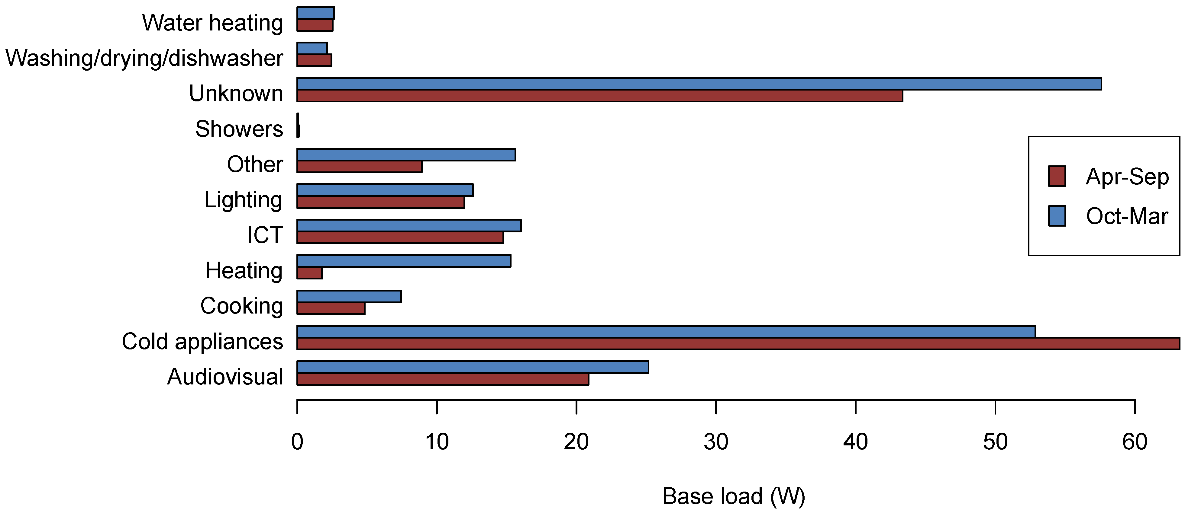
The majority of known domestic base load power is used to run fridges and freezers, which on average account for more than two-fifths of the total. Even during the winter, when the ambient temperatures are more favourable, these appliances remain the largest component of base load. This means that improvements in the efficiency of cold appliances have the potential to make a larger impact on base load power than interventions to other appliances.

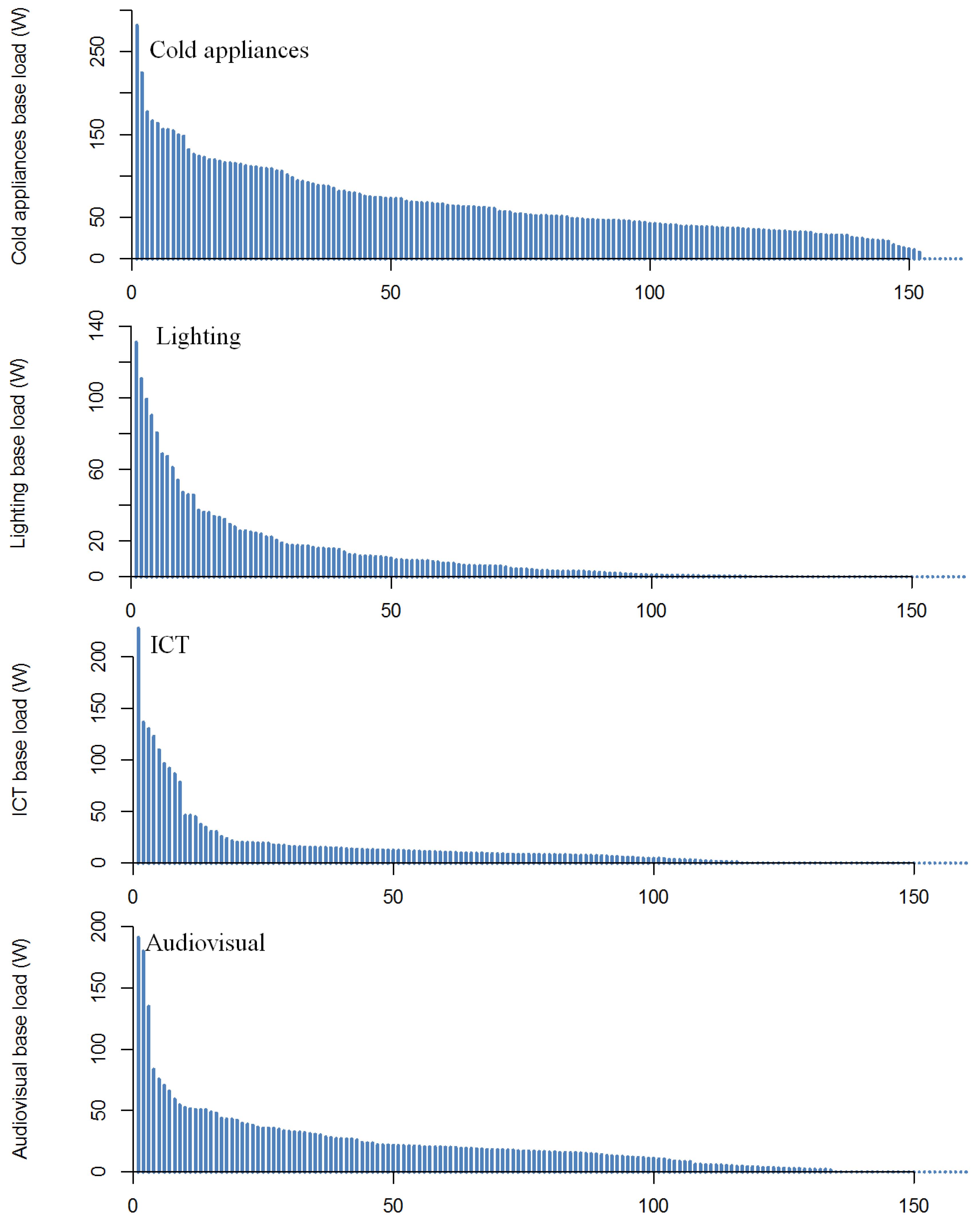
For a few appliance categories, relatively small numbers of homes were found to account for a large share of the base load power demand. For example, 17% of homes account for 71% of the total lighting base load, and there are similar skewed distributions for audiovisual and ICT base load electricity use. This suggests that, for these appliances, if policymakers wished to reduce base load power use (for instance, to allow for more overnight charging of electric vehicles, or overnight use of heat pumps), interventions targeting the key high-use households would be particularly effective—if these could be identified. By contrast, the base load for some uses, most notably cold appliances, were found to have a more uniform distribution.

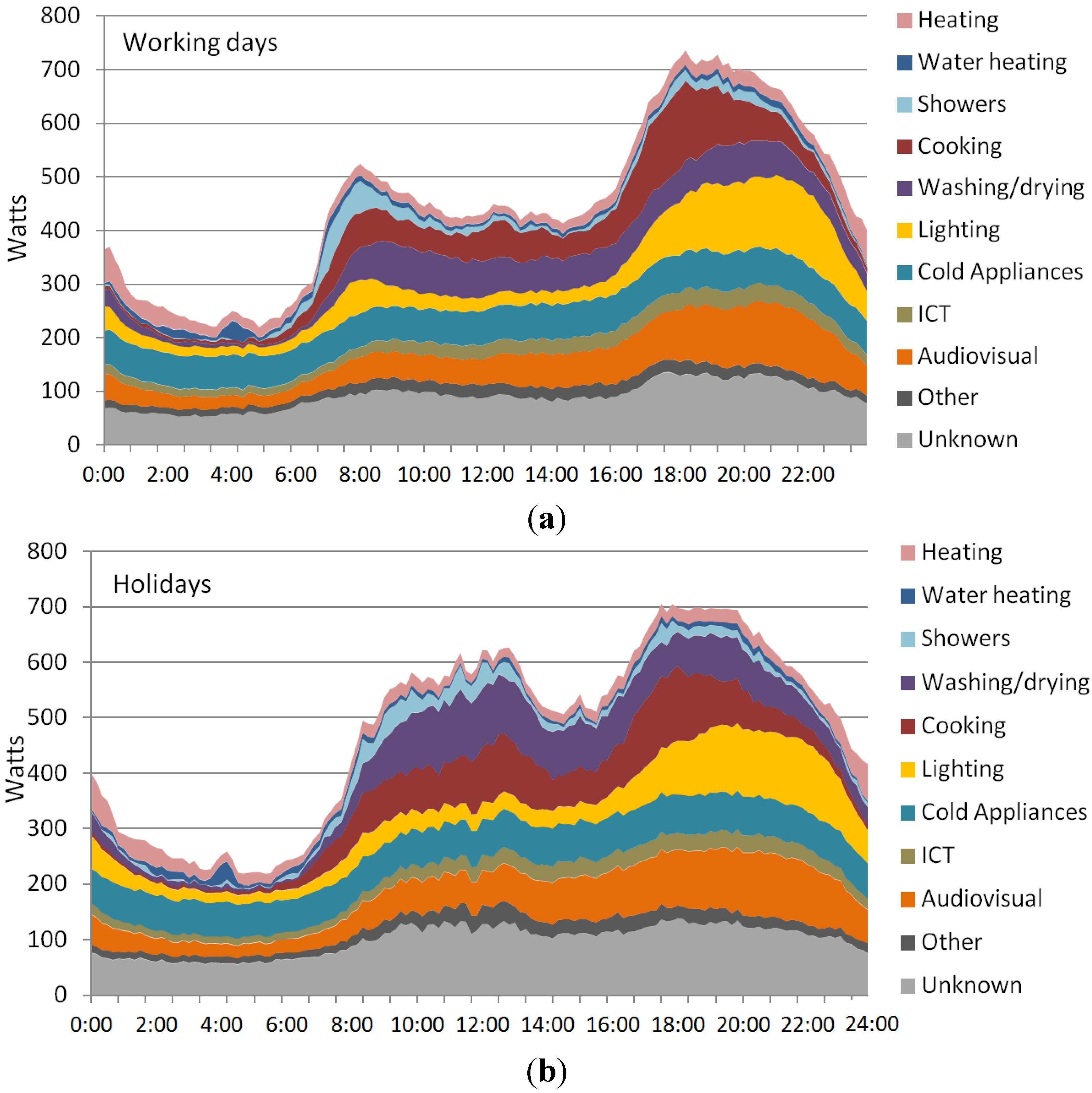
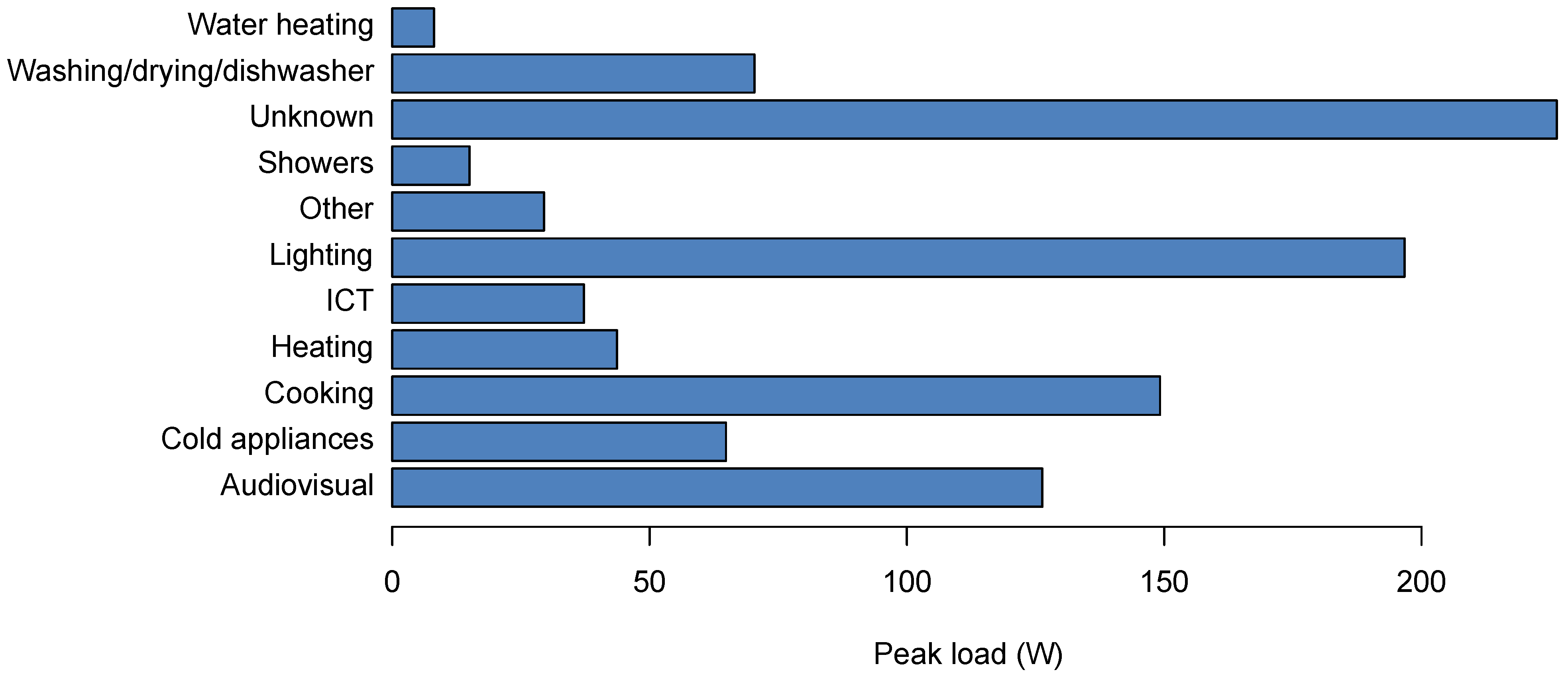
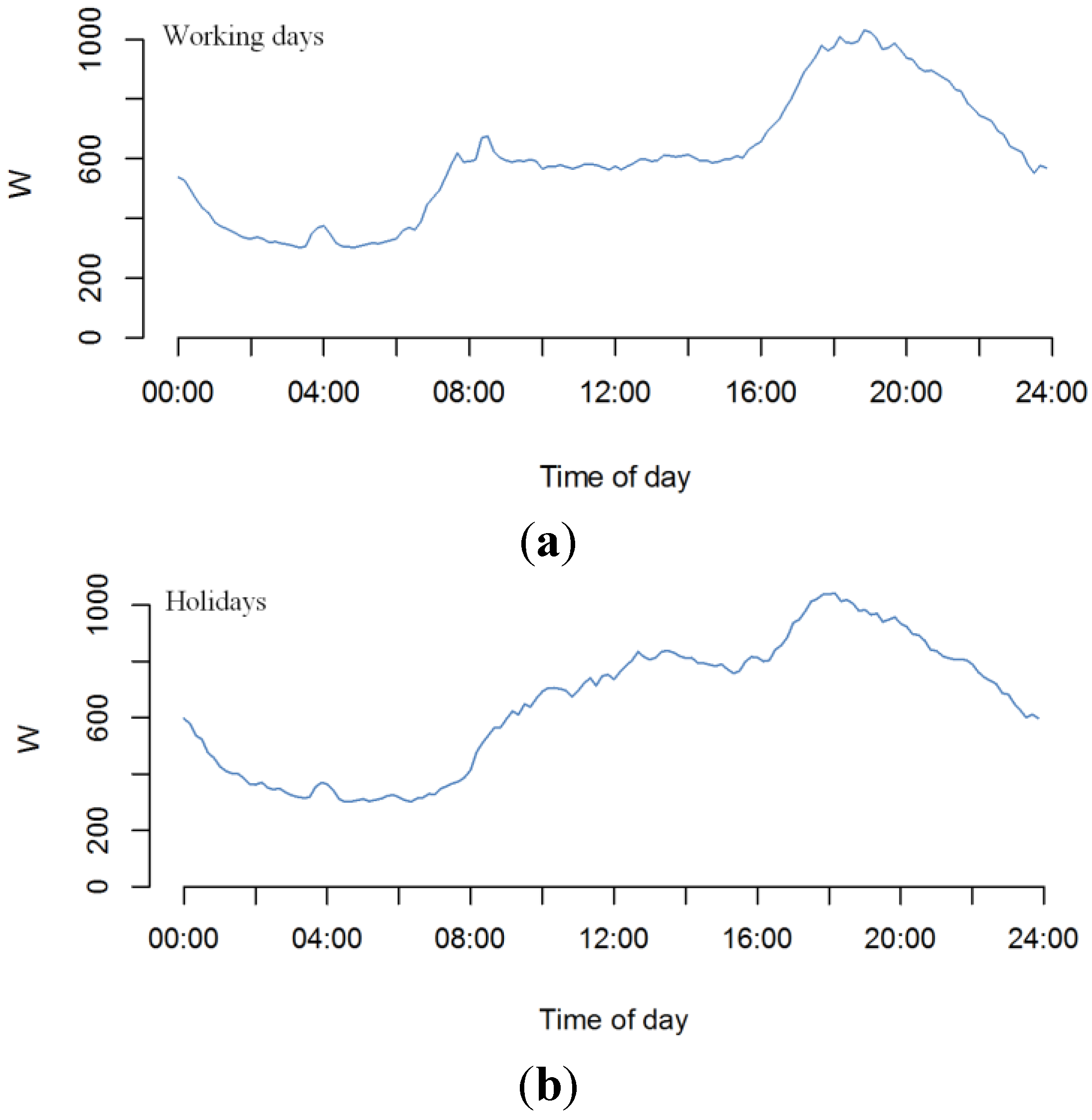
Average peak electricity use for the sample was from 6 p.m. to 7 p.m. in winter, with a mean of 970 Watts per household. The largest share of known electricity use at this time was lighting, cooking and audiovisual appliances, which unfortunately are all hard to shift to other times of day. Consequently, substituting more efficient appliances, and particularly more efficient lighting, would make a bigger difference than “peak load” interventions per se.

There is the potential for shifting the time of use of washing appliances, for instance using timers. However, there have been concerns about fire safety when using these appliances overnight [33], and the analysis suggests that the potential savings are small: on average wet appliances account for only 7% of domestic peak power. There is also the potential for using smart cold appliances (notably controls based on frequency response, which automatically cut out for short periods when there is high power demand on the grid), but again the potential savings are likely to be small (possibly less than 3% of peak power [34]). Although load shifting of this scale may not have large impacts for individual households, aggregated to the regional or national scale the benefits for utilities providers may be important.

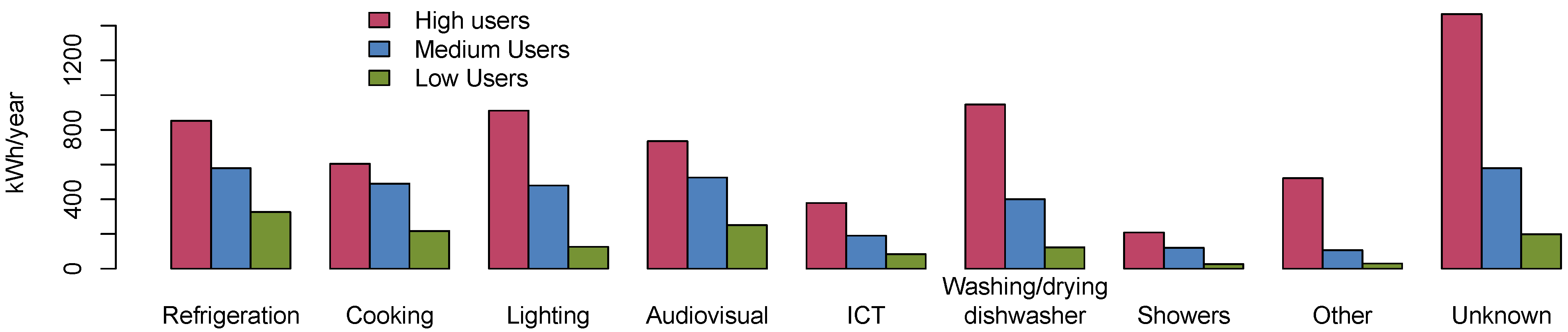
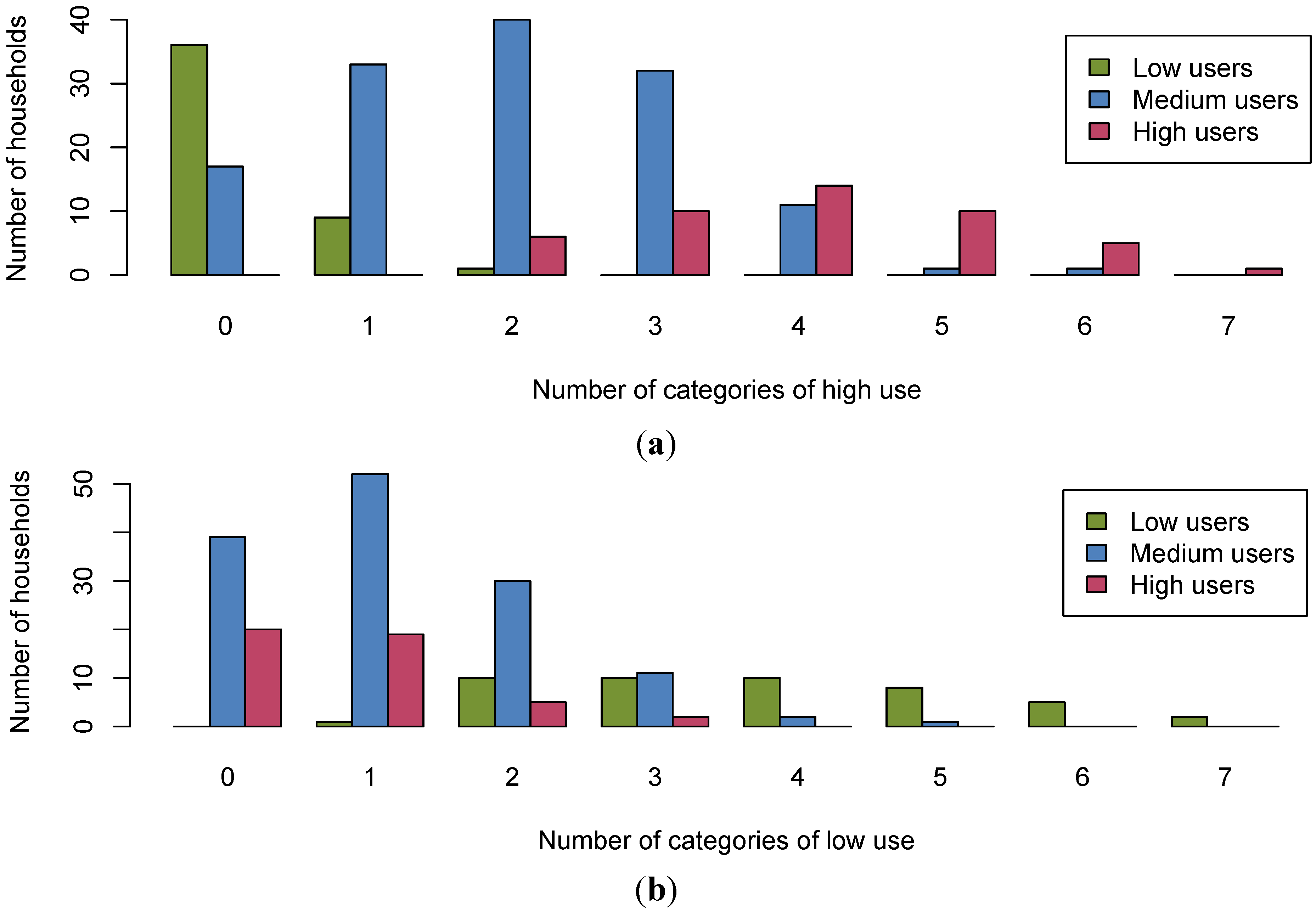
The characteristics of high and low energy consuming households were examined, both at the scale of overall electricity use, and the different appliance groups. The reasons for high and low use were found to be both varied and complex. High consuming households typically exhibited high consumption across a number of appliance groups but, significantly, rarely all of them. Consequently, reducing electricity use among high users would require identifying and making improvements across a range of different appliance types in each home. Even the low-use households were very seldom low in every appliance category-typically they were in two to five categories, and some high-use households were found to demonstrate low use in some areas.

This has implications for policy: instead of simply encouraging generic, blanket improvements to all forms of electricity use in high-consuming dwellings, it may be more effective to provide information, incentives, grants or other appropriate interventions targeted at specific high-use appliance characteristics. There may also be a case for enabling householders to compare their use of electricity for specific appliance types with their peers. Many studies have found that such comparisons, and the spirit of competition they help to engender, can be effective in helping to reduce total energy use [35,36]. Potentially, comparisons of energy use for specific appliances may help to prompt savings, especially if householders see that they have particularly high energy use compared to their peers.

Unfortunately, the fact that overall dwelling energy use does not necessarily indicate energy performance at the scale of the individual appliances, highlights the difficulty households may have in making improvements based solely on metering installed at the distribution board. Without understanding the internal breakdown of uses (for example through appliance-scale metering, or by switching appliances on and off with distribution-level smart metering), it may be difficult to identify the most appropriate improvement measures for each home. A related issue that further complicates research in this field is the enormous range in energy use for individual appliance types. For example, a more than tenfold variation was observed, between the highest and lowest HES energy consumers for audiovisual appliances and electric showers.

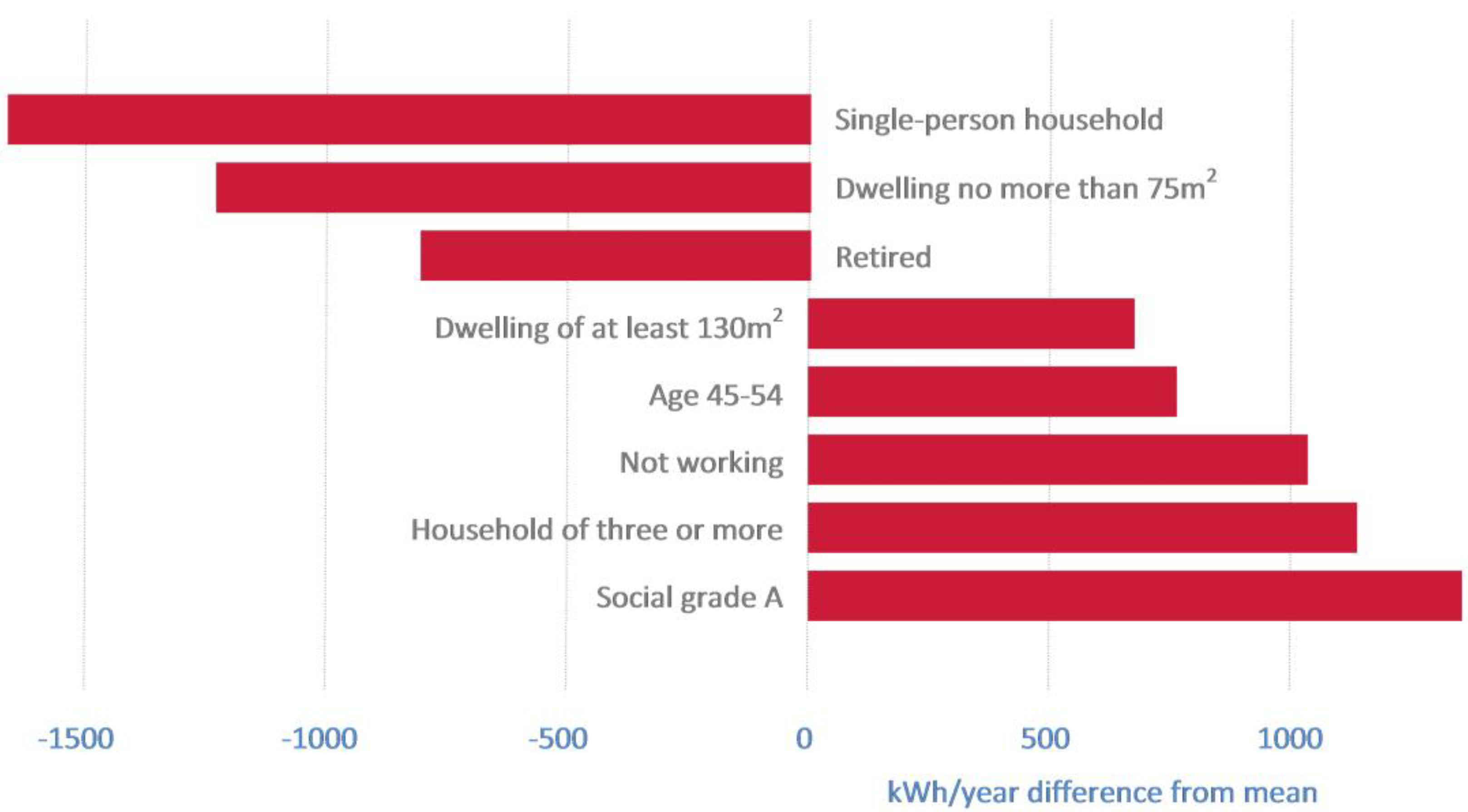
The results of the multi-variate analysis identified different demographic variables correlating with variations in household electricity use. The analysis suggests that working households have lower energy use for audiovisual appliances than other households of working age. It also indicates that energy use for lighting is highest among the highest social grades. More empirical work is needed to further explore the drivers for residential energy performance, and the multi-variate analysis is somewhat stymied by small samples.

The absence of income data for the HES households means that it is not possible to compare the results directly with past studies that have shown that income is a major driver of electricity use. However, a number of the variables examined, like dwelling size and social grade, may be indirect indicators for income suggesting that income is important. Dwelling size and the number of occupants did emerge from the analysis as important factors, consistent with past research [15,16,17]. Furthermore, the findings from this paper are consistent with those of past work investigating the links between total electricity use and energy use for individual appliances [22].

The HES survey had limitations, some of which have been mentioned already. Two of the biggest were the modest sample size and the inability to go back to the participants, following the monitoring, to examine why they used electricity as they did, or to explore how energy consumption could be reduced. (Indeed, the consent forms used during the survey specifically precluded follow-on interviews for most households.) The authors advocate further research work in this area, on greater numbers of households, alongside qualitative interviews and time-use diaries to give a more complete understanding of electricity use in homes.

Further work could also explore how biases in the HES sample impact on how representative the findings are of the overall domestic stock. In total, for 2011, the mean annual electricity use for the HES sample was within 1.5% of the UK average. It is likely that the omission of private rented and social housing from the sample distorts the data. A recent study found that owner-occupied homes use almost 14% more electricity than privately rented homes, which in turn use 8% more than social housing [17], suggesting that the HES results may overestimate the average performance of the overall stock. However, more research is required to better understand the different patterns of electricity use at the scale of specific appliances, which have been found to vary with tenure [21]. Furthermore, the drivers of these differences may be complex. For example, income and employment trends could impact indirectly on energy use, by correlating to variations in the average age of appliances in rented, as opposed to owner-occupied, homes. The HES bias towards households that are slightly more energy conscious than average is possibly less important than the difference in tenure. However, further empirical research could shed more light on any disparities.

Let us return to the title, “What can we learn from the Household Electricity Survey?” The depth and breadth of data gathered in the HES has presented a unique opportunity to improve the understanding of how electricity is used in contemporary UK homes. The paper highlights some of the potential that monitoring exercises have in quantifying the drivers for energy performance and how to relate this to policy issues. Despite the complexity of undertaking large-scale, long-term, detailed surveys like the HES, robust collection and analysis of actual household energy data is a key part of identifying the potential that the sector has for carbon emissions reductions, both for the UK and abroad.

References

1. Energy Efficiency Indicators: Fundamentals on Statistics; International Energy Agency: Paris, France, 2014.
2. Perez-Lombard, L.; Ortiz, J.; Pout, C. A review on buildings energy consumption information. Energy Build. 2008, 40, 394–398. [Google Scholar] [CrossRef]
3. Palmer, J.; Cooper, I. United Kingdom Housing Energy Fact File 2013; Department of Energy and Climate Change (DECC): London, UK, 2014.
4. UK Parliament. Climate Change Act 2008; Her Majesty’s Stationery Office (HMSO): London, UK, 2008.
5. UK Greenhouse Gas Emissions Performance Against Emissions Reduction Targets 2012: Provisional Figures; Department of Energy and Climate Change (DECC): London, UK, 2013.
6. 2012 Guidelines to DEFRA/DECCs GHG Conversion Factors for Company Reporting; AEA: London, UK, 2012.
7. Electricity Capacity Assessment Report 2013; Office of Gas and Electricity Markets (Ofgem): London, UK, 2013.
8. Zimmermann, J.; Evans, M.; Griggs, J.; King, N.; Harding, L.; Roberts, P.; Evans, C. Household Electricity Survey: A Study of Domestic Electrical Product Usage; Intertek Testing and Certification Ltd.: Milton Keynes, UK, 2012. [Google Scholar]
9. Owen, P. Powering the Nation: Household Electricity-Using Habits Revealed; Energy Saving Trust: London, UK, 2012. [Google Scholar]
10. Palmer, J.; Terry, N. Powering the Nation 2: Electricity Use in Homes, and How to Reduce It; Department of Energy and Climate Change (DECC): London, UK, 2014.
11. Energy Consumption in the UK (Tables 3.1 and 3.3); Department of Energy and Climate Change (DECC): London, UK, 2012.
12. Zimmermann, J. End-Use Metering Campaign in 400 Households in Sweden: Assessment of the Potential Electricity Savings; Enertech: Eskilstuna, Sweden, 2009. [Google Scholar]
13. Thornton, A. Public Attitudes and Behaviours Towards the Environment-Tracker Survey: A Report to DEFRA; Department for Environment, Food & Rural Affairs (DEFRA): London, UK, 2009.
14. Live Tables on Dwelling Stock; Department of Communities and Local Government: London, UK, 2012. Available online: https://www.gov.uk/government/statistical-data-sets/live-tables-on-dwelling-stock-including-vacants (accessed on 10 July 2014).
15. Newborough, M.; Augood, P. Demand-side management opportunities for the UK domestic sector. IEEE Proc. 1999, 146, 283–293. [Google Scholar] [CrossRef]
16. Druckman, A.; Jackson, T. Household energy composition in the UK: A highly geographically and socio-economically disaggregated model. Energy Policy 2008, 36, 3177–3192. [Google Scholar] [CrossRef] [Green Version]
17. Wyatt, P. A dwelling-level investigation into the physical and socio-economic drivers of domestic energy consumption in England. Energy Policy 2013, 60, 540–549. [Google Scholar] [CrossRef]
18. Yohanis, Y.; Mondol, J.; Wright, A.; Norton, B. Real-life energy use in the UK: How occupancy and dwelling characteristics affect domestic electricity use. Energy Build. 2008, 40, 1053–1059. [Google Scholar] [CrossRef]
19. Wiesmann, D.; Azevedo, I.L.; Ferrao, P.; Fernandez, J. Residential electricity consumption in portugal: Findings from top-down and bottom-up models. Energy Policy 2011, 39, 2772–2779. [Google Scholar] [CrossRef]
20. De Almeida, A.; Fonseca, P.; Schlomann, B.; Feiberg, N. Characterisation of the households electricity consumption in the EU, potential energy savings and specific policy recommendations. Energy Build. 2011, 43, 1884–1894. [Google Scholar] [CrossRef] [Green Version]
21. Hulme, J.; Beaumont, A.; Summers, C. Energy Follow-Up Survey 2011: Report 9-Domestic Appliances, Cooking & Cooling Equipment; Building Research Establishment (BRE): Watford, UK, 2013. [Google Scholar]
22. Firth, S.; Lomas, K.; Wright, A.; Wall, R. Identifying trends in the use of domestic appliances from household electricity consumption measurements. Energy Build. 2008, 40, 926–936. [Google Scholar] [CrossRef] [Green Version]
23. Haines, V.; Lomas, K.; Thomson, M.; Richardson, I.; Bhamra, T.; Giulietti, M. How Trends in Appliances Affect Domestic CO2 Emissions: A Review of Home and Garden Appliances; Department of Energy and Climate Change (DECC): London, UK, 2010.
24. Johnston, D.; Lowe, R.; Bell, M. An exploration of the technical feasibility of achieving CO2 emission reductions in excess of 0% within the UK housing stock by the year 2050. Energy Policy 2005, 33, 1643–1659. [Google Scholar] [CrossRef]
25. Hughes, M.; Palmer, J.; Cheng, V.; Shipworth, D. Sensitivity and uncertainty analysis of England’s housing energy model. Build. Res. Inf. 2013, 41, 156–167. [Google Scholar] [CrossRef]
26. Pout, C.; MacKenzie, F.; Olloqui, E. The Impact of Changing Energy Use Patterns in Buildings on Peak Electricity Demand in the UK; Building Research Establishment (BRE): Watford, UK, 2008. [Google Scholar]
27. Additional Investigation of Data from the Household Electricity Survey: Comparison with the NEED Database and with Electricity Demand Profiles From National Grid; Department of Energy and Climate Change (DECC): London, UK, 2014.
28. Newsham, G.; Bowker, B. The effect of utlity time-varying pricing and load control strategies on residential summer peak electricity use: A review. Energy Policy 2010, 38, 3289–3296. [Google Scholar] [CrossRef]
29. Zehir, M.; Bagriyanik, M. Demand side management by controlling refrigerators and its effects on consumers. Energy Convers. Manag. 2012, 64, 238–244. [Google Scholar] [CrossRef]
30. Boardman, B. Low Energy Lights Will Keep the Lights on. In Proceedings of the Radical Emissions Reduction Conference, London, UK, 11 December 2013.
31. Terry, N.; Palmer, J.; Godoy-Shimizu, D.; Firth, S.; Kane, T.; Tillson, A. Further Analysis of the Household Electricity Survey: Lighting Study (Final Report); Department of Energy and Climate Change (DECC): London, UK, 2013.
32. Burnham, K.; Anderson, D. Model Selection and Multimodel Inference: A Practical Information-Theoretic Approach, 2nd ed.; Springer-Verlag: New York, NY, USA, 2002. [Google Scholar]
33. Kitchen Appliance Warning After Bearstead Fire. BBC, 2010. Available online: http://www.bbc.co.uk/news/uk-england-kent-11424687 (accessed on 10 July 2014).
34. Palmer, J.; Terry, N.; Kane, T. Further Analysis of the Household Electricity Survey-Early Findings: Demand Side Management; Department of Energy and Climate Change (DECC): London, UK, 2013.
35. Ehrhardt-Martinez, K.; Donnelly, K.; Laitner, J. Advanced Metering Initiatives and Residential Feedback Programs: A Meta-Review for Household Electricity-Saving Opportunities; No. E105; American Council for an Energy-Efficient Economy: Washington, DC, USA, 2010. [Google Scholar]
36. Ayres, I.; Raseman, S.; Shih, A. Evidence from Two Large Field Experiments that Peer Comparison Feedback Can Reduce Residential Energy Usage; National Bureau of Economic Research: Cambridge, MA, USA, 2009.