Modeling of Microstructure Evolution of Ti6Al4V for Additive Manufacturing

International Center for Numerical Methods in Engineering (CIMNE), Universidad Politécnica de Cataluña (UPC), Edificio C1, Campus Norte, Gran Capitán s/n, 08034 Barcelona, Spain
*
Author to whom correspondence should be addressed.
Metals 2018, 8(8), 633; https://doi.org/10.3390/met8080633
Submission received: 14 June 2018
/
Revised: 1 August 2018
/
Accepted: 6 August 2018
/
Published: 10 August 2018
Abstract
:AM processes are characterized by complex thermal cycles that have a deep influence on the microstructural transformations of the deposited alloy. In this work, a general model for the prediction of microstructure evolution during solid state transformations of Ti6Al4V is presented. Several formulations have been developed and employed for modeling phase transformations in other manufacturing processes and, particularly, in casting. The proposed model is mainly based on the combination and modification of some of these existing formulations, leading to a new overall model specifically dedicated to AM. The accuracy and suitability of the integrated model is enhanced, introducing new dedicated features. In fact the model is designed to deal with fast cooling and re-heating cycles typical of AM processes because: (a) it is able to consider incomplete transformations and varying initial content of phases and (b) it can take into account simultaneous transformations.The model is implemented in COMET, an in-house Finite Element (FE)-based framework for the solution of thermo-mechanical engineering problems. The validation of the microstructural model is performed by comparing the simulation results with the data available in the literature. The sensitivity of the model to the variation of material parameters is also discussed.
1. Introduction
Compared to traditional forming processes, AM metal deposition is characterized by successive thermal cycles with unusual ranges of cooling and heating conditions. According to the process parameters and to the deposition strategy, these thermal cycles present different ranges of temperatures in each point of the part. The local thermal cycles are also strongly influenced by the distance from the heat source, which is continuously moving according to the metal deposition sequence. The complex temperature evolution directly influences the kinetics of microstructure formations during the solidification and the solid state transformations. As the thermal environment is not constant, the resulting microstructures are inhomogeneous despite constant manufacturing parameters [1]. In fact, peripheral areas of the deposited metal present different thermal conditions if compared with massive areas, causing differences in the grain orientation and size. The high cooling rates, typical of fast AM thermal cycles, can lead to the formation of metastable martensitic structures. However, due to the heat accumulation during the successive depositions, a bulk temperature increment can take place, allowing for partial or complete martensite dissolution. This leads to unique microstructural and mechanical properties, different from cast or wrought parts obtained from identical alloy compositions [2]. If compared with casting, parts obtained by AM are usually characterized by finer microstructure due to high cooling rates. On one hand, finer microstructure can lead to higher tensile properties, on the other hand, typical AM defects such as microporosity and oxide inclusions can cause a decrease of elongation at break [1,3,4]. The evaluation of local mechanical properties of parts obtained by metal deposition is one of the main challenges when modeling AM processes. The correlation between microstructure and mechanical properties is an effective approach to this industrial requirement. Data for these empirical correlations can be found in the literature for most of the alloys employed in mechanical applications (such as for Ti6Al4V [5]) but a dedicated work of characterization is still to be done for several others alloys.
In this work, a model for the prediction of microstructure evolution of Ti6Al4V during AM processes is presented. The main phase evolutions that take place during the solid state transformations of Ti6Al4V are considered, both for cooling and re-heating conditions. A phenomenological approach is employed, allowing to directly correlate the local temperature-time curves with the evolution of the phase fractions. The models considered for each specific phase transformation are similar to the ones used for similar processes such as welding, casting or heat treatments. Medium-slow diffusional phase transformations are modeled by means of Johnson-Mehl-Avrami-Kolmogorov (JMAK) equations [6], using the additivity rule [7] and considering the Temperature-Time-Transformation (TTT) curves as material data input. In the case of fast diffusionless transformations (such as martensite formation), empirical evolution laws are employed [8,9].
The model is specifically designed in order to take into account the typical conditions of AM processes. During these processes, heating and cooling transformations take place several times due to the thermal cycles generated by the layer-by-layer metal deposition sequence. Most of the times, these cycles are so fast that the transformations remain incomplete. Dedicated algorithms that switch on and off each transformation according to the AM process conditions, taking into account incomplete transformations and varying initial fractions for each transformation, are considered very rarely in the literature [10,11]. In this paper, additional features are introduced, such as simultaneous transformations as well as the martensite accumulation throughout the cycles. The microstructural model is validated comparing the simulations results with experimental or numerical data available in the literature.
The model has been implemented in COMET, a Finite Element (FE)-based framework used for the thermo-mechanical simulation of metal deposition processes [12,13,14]. Using COMET, the welding path is modeled by means of an ad-hoc activation methodology that switches on the elements according to the scanning sequence. The numerical results of temperature evolution during the AM process provide the thermal inputs to predict the microstructure in each point of the part.
Therefore, the objective of this work is to enhance the numerical simulation of AM by developing and calibrating dedicated models for the microstructure evolution of Ti6Al4V.
The outline of the paper is as follows. In Section 2, a short review of the state-of-the-art of microstructural modeling for Ti6Al4V is reported. In Section 3, the overall formulation of the microstructural model specifically developed for AM processes is given. In Section 4, the sensitivity analysis of the model to material data for different conditions is reported. Finally, a work of validation of the model for 3D microstructural simulations of AM with different process parameters is presented.
2. Microstructure Evolution of Ti6Al4V
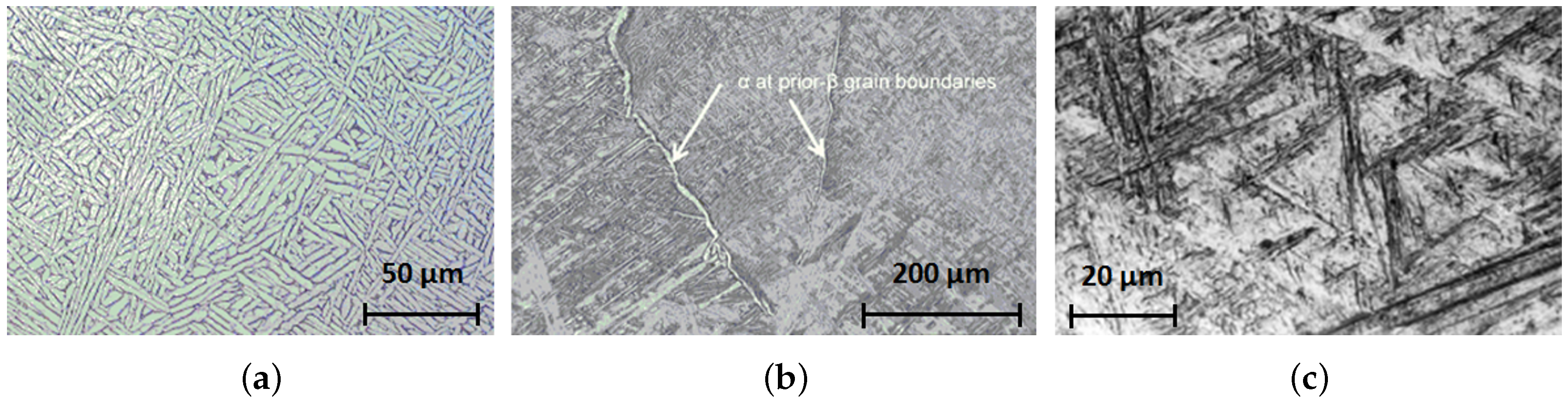
Depending on the temperature evolution, titanium can present two main crystal structures: the beta phase (), a Body-Centred Cubic (BCC) structure stable at high temperatures, and the alpha phase (), an Hexagonal Close-Packed (HCP) structure stable at low temperatures and normally present at room temperature. During the cooling of liquid titanium alloys, grains start to nucleate and grow. After the complete solidification, the solid state transformation from to takes place. In Ti6Al4V alloys, the Vanadium acts as stabilizer element, allowing for the presence of a little stable fraction of phase at room temperature. Hence, at room temperature, Ti6Al4V alloy is characterized by a mix of phases that can show a large variety of microstructures and features depending on the thermal cycles experienced. The most typical microstructures of Ti6Al4V alloys are shown in Figure 1 [15,16]:
- -
- Widmanstätten structure (Figure 1a): It is composed by lamellae, with a small retained amount of intra-lamellar , enriched by vanadium, typical of slow-medium cooling rates. lamellae are usually aligned to form colonies. A slight variant of this structure, characterized by thinner lamellae, is called “basket-weave” structure. In this work, no difference is made between these two structures and we will refer to them as Widmanstätten structures.
- -
- Grain boundary (Figure 1b): an allotriomorph crystal structure generally located at the grains boundaries.
- -
- Martensite (Figure 1c): it is a non-equilibrium phase with acicular shape similar to small needles, typical of fast cooling rates. There exists a variant of this structure called massive alpha, typical of medium-fast cooling rates, but, in this work, this difference is not considered. Both Martensite and Massive alpha present HCP crystal structure.
For the sake of simplicity, in the following the structural components described above will be referred to as phases even if is not the proper metallurgical terminology.
According to Charles and Lindgren [10], during the cooling of Ti6Al4V, three different main transformations take place: solidification of phase from the liquid, solid state transformation and martensite formation.
Below liquidus temperature, phase starts to form. Depending on the cooling conditions, grains can show equiaxed or columnar morphologies [17].
Following the cooling, when the -transus temperature (around 995–1000 °C) is reached, the phase starts to form from the previous phase. Generally, slow cooling rates lead to Widmanstätten structures. The diffusion-controlled transformation can be modeled by means of a Johnson-Mehl-Avrami-Kolmogorov (JMAK) equation [6], using the additivity rule [7]. JMAK equations are defined by temperature-dependent parameters that can be extracted from Temperature-Time-Transformation (TTT) curves. The lath thickness is inversely proportional to the cooling rate and it can be modeled by an empirical Arrhenius equation [18,19].
In case of faster cooling rates, martensite can form from the residual still available once reached the martensite start temperature (around 650–500 °C). This transformation is considered diffusionless and can be modeled using the Koistinen-Marburger law, an empirical relationship which depends on the undercooling with respect to [8]. Note that if the transformation of into is complete, then no fraction is available for the martensitic transformation.
In the case of reheating, three different transformations can occur: dissolution of martensite into , transformation of into and remelting of .
The martensite is a metastable structure that tends to re-transform, at high temperature and given sufficient time, to more stable structures similar to the Widmanstätten microstructure. In several models, these new structures are generally referred to as Widmanstätten structures [15]. In [20], Gil Mur proposes to model the transformation with JMAK equations using the same additivity rule principle proposed for the Widmanstätten formation. An inverse correlation between hardness and martensite content in Ti6Al4V is also proposed. Then, from the evolution of the hardness in martensitic samples reheated at different levels of temperature, it is possible to extract the experimental parameters to characterize the JMAK equations to model the martensite dissolution. This transformation starts at low temperatures: the martensite dissolution start temperature is around 350–400 °C (see [20]).
During heating, above the transus temperature (600–650 °C), the total alpha phase () starts to re-transform into phase. Considering the high heating rates of AM processes, transformation can be approximated (together with the re-melting of ) as an instantaneous transformation which follows the equilibrium phase diagram [21]. However, other approaches for recovering have been adopted in literature, such as the additivity rule with JMAK equations or a temperature dependent parabolic law as proposed by Kelly [9].
3. Microstructure Evolution Model
3.1. General Formulation for Diffusion-Controlled Transformations
The classical JMAK model, as well as those modifications necessary to consider the incomplete transformations and the existence of initial phase fractions, are presented in this section. The inverse formulation to define the empirical parameters needed by the JMAK equations is shown. Next, the principle of additivity rule is detailed.
3.1.1. Johnson-Mehl-Avrami-Kolmogorov Equation
The JMAK (Johnson-Mehl [22]-Avrami [6]-Kolmogorov [23]) formulation is used to model diffusion-controlled transformations. Typically, a sigmoidal (or s-shaped) time evolution of the transformation starts slowly, continues relatively fast and slows down again at the end of the transformation. This function suits the typical phases formation: nucleation, growth and grain impingement.
The following form of the JMAK model [6] describes a complete evolution of a generic phase fraction X from 0 to 1:
where are material parameters which control the duration and the speed of the transformation and t is the time from the start of the considered transformation. Two JMAK phase evolution calculated with different parameter are shown in Figure 2 (red and blue dashed lines). The same evolution law can be written in rate form by differenciating Equation (1):
3.1.2. The TTT Curves
The parameters k, p that define the kinetics of phase evolution at each temperature are extracted from TTT (Temperature-Time-Transformation) curves. These curves are obtained experimentally measuring the evolution of the different phases under isothermal treatment repeated at different temperatures. Two conventional values (e.g., and ) define the initial and final measured fractions , respectively. Hence, the TTT curves represent the initial and final times of isothermal transformations at given temperatures as shown in the bottom right of Figure 2.
In this work, piecewise linear functions have been used to describe the TTT curves. Hence, for a given temperature T, 2 equations can be written corresponding to the initial and final fraction of each phase using Equation (1):
From these, the parameters of the JMAK transformations are obtained as:
where:
3.1.3. Additivity Rule
The JMAK formulation was originally employed to describe isothermal transformations for heat treatment processes. In this case, coefficients characterize the kinetics of nucleation and grain growth at a prescribed constant temperature T. However, during the fast thermal cycles typical of AM processes, the transformations are not isothermal. For this reason, the formulation has to be adapted to non-isothermal transformations by introducing the additivity rule [7].
According to this rule, the actual temperature evolution is replaced by the sum of consecutive isothermal time increments. Different phase evolution kinetics are associated to each isothermal time step using JMAK equations defined by the parameters at the respective temperature value. Hence, the overall phase evolution is computed by summing the contribution of the fractions calculated for each isothermal step.
The application of the additivity rule requires the computation of an equivalent time at the beginning of each time increment in order to account for the change of the temperature dependent parameters . The situation is illustrated in Figure 2. At time , a change of temperature occurs, from to . Phase evolution before has been evaluated with parameters and ; phase evolution after has to be evaluated with parameters and . As phase kinetics Equation (1) is expressed in total, rather than rate, form, an equivalent time is defined so that:
this being:
Note that only depends on and , but not on the parameters defining phase evolution prior to . Using the equivalent time , the phase fraction at time is calculated as:
Alternatively, Equation (2) in rate form can be used to evaluate the phase fraction increment as:
and then to update . This does not require the computation of the equivalent time when a forward Euler integration algoritm is used.
3.1.4. Modified JMAK Model Accounting for Initial Phase Fractions and Incomplete Transformations
The original JMAK model [6] describes a complete transformation of phase 1 into phase 2. During the transformation, fraction of phase 1 decreases from 1 to 0 while fraction of phase 2 evolves from 0 to 1 (). However, during the solid state transformations that take place in AM processes of Ti6Al4V alloys, the metallurgical phenomena can be more complex than a single complete transformation. In fact, due to the previous thermal cycles, some minor phases or structural constituents may not participate to the main transformation, reducing the available initial fraction of phase . Moreover, transformations may be incomplete. For instance, according to the phase diagram of Ti6Al4V, the transformation is never completed because a small amount of is left even at room temperature.
In order to consider these phenomena, the original JMAK formulation in (1) is modified [10]:
where is the initial available fraction of phase 1 at the beginning of the reaction and is the fraction of phase 2 that can form at equilibrium state at the considered temperature. The value of initial depends on the phase changes during the previous transformations, while can be extracted from the equilibrium phase diagrams of the alloys.
3.2. Microstructure Modeling of Ti6Al4V for AM Processes
The microstructural model used in this work is presented next. The model has been implemented in COMET, a Finite Element (FE)-based framework used for the thermo-mechanical simulation of metal deposition processes [12,13,14].
The following 4 main solid state transformation for Ti6Al4V alloy are considered:
- (I)
- Formation of Widmanstätten : diffusion-controlled transformation () for cooling processes below the -transus temperature .
- (II)
- Formation of Martensite : diffusionless transformation () for fast cooling processes below the martensite temperature .
- (III)
- Dissolution of Martensite : diffusion-controlled transformation ( → ) by heating process above .
- (IV)
- Dissolution of total (or re-formation of ): diffusionless transformation ( → ) by heating process above .
In Figure 3 a schematic representation of the cooling/heating condition and temperature ranges typical of these transformations is shown. The arrows represent the temperature rates that take place during the AM processing: cooling (blue) or heating (red). The single-line arrows correspond to diffusion-controlled transformations, the double-line arrows correspond to diffusionless transformations. Note that the dissolution of martensite happens during heating but it may take place also during isothermal treatments and even during very slow cooling at temperature above .
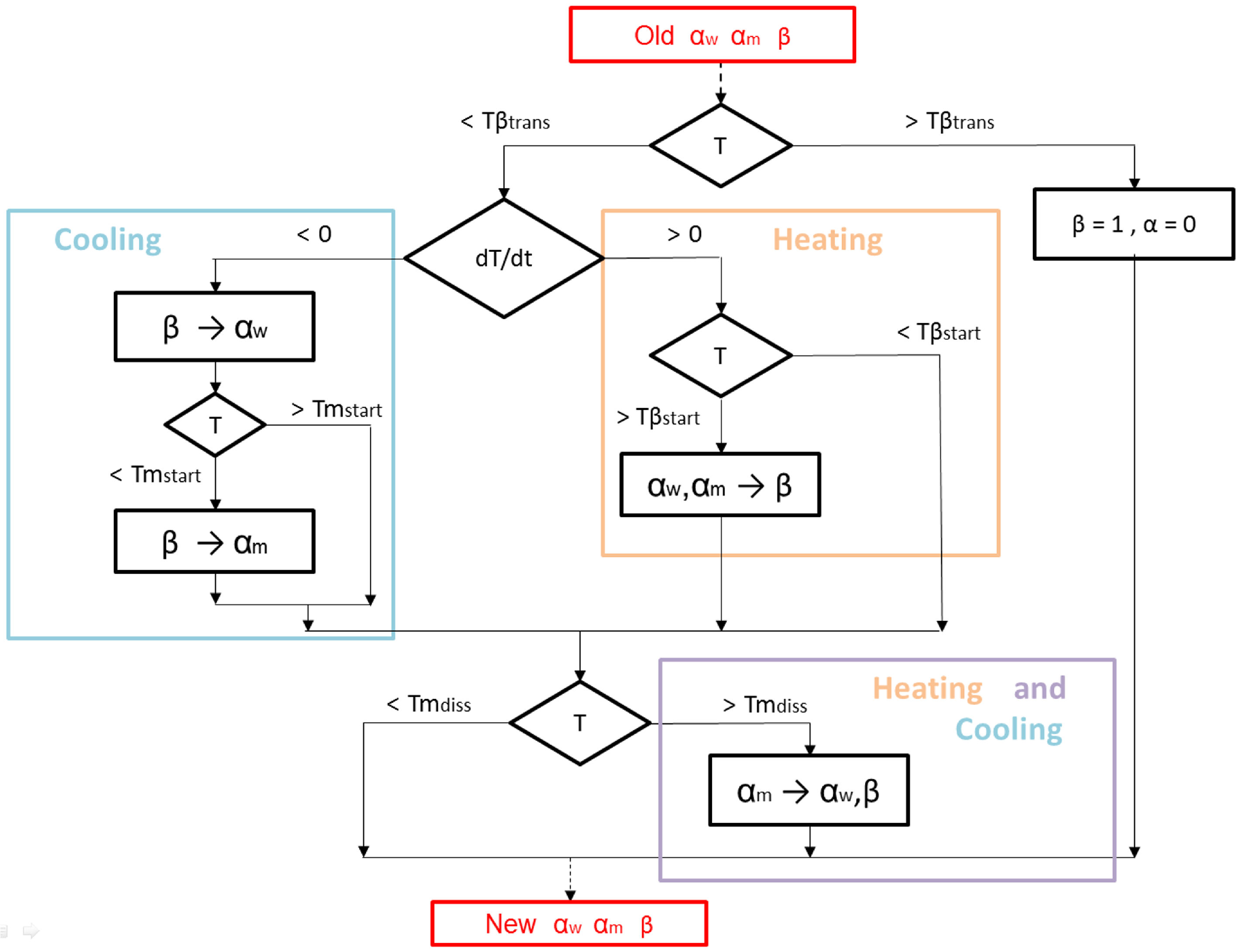
The required input of the model is the temperature evolution of the alloy. If the thermal history of an entire domain is available, the microstructure modeling is performed locally at each material point. The temperature evolution is split into a sequence of time steps . Both temperature and cooling/heating rate are evaluated according to the algoritm proposed in Figure 4 in order to establish which transformations will take place.
For each time step, the algorithm manages the sequential computation of different transformations taking place simultaneously. The increments of fractions () are computed for each transformation as . (or alternatively using Equation (11). These increments are used to update the phase fractions at the end of the overall algorithm only, making possible to consider contemporary transformations.
As each transformation is considered separately, contemporary transformations with the same starting phase (e.g., ) and different forming phases (e.g., , ) can potentially lead to an excessive consumption of the starting phase. To avoid this, the available amount of starting phase is proportionally shared between the two transformations by rescaling the incremental phase changes as:
For example, this strategy allows the model to consider the simultaneous transformation of into and which can occur for intermediate cooling rates [24].
3.2.1. Formation of Alpha Widmanstätten
The formation of is calculated for each time step using the modified JMAK formulation in Equation (12) and following the additivity rule. The fraction at the equivalent time at temperature T (and then its increment ) is calculated as in Equation (13):
where , are the JMAK parameter of formation at the temperature T of the isothermal time step, is the available fraction of beta phase at the beginning of the reaction and is the fraction that can form according to the phase diagram of the alloy at temperature T. is the equivalent time that is needed to reach the amount of phase at the end of the previous time step according to the evolution law of the actual isothermal step. As for Equation (14), is defined as:
Note that the available fraction of beta phase at the beginning of the reaction depends on the previous thermal history of the process. If the alloy has suffered fast cooling, the available is reduced by the presence of . Due to mass conservation (), for each time step can be written as: , where are the fractions at the previous time step. Note that is not involved in this transformation.
3.2.2. Formation of Alpha Martensite
In case of fast cooling rates and temperatures below the martensite start temperature , the residual phase still available can transform into martensite or massive . Due to its fast formation, is a non-equilibrium phase and its evolution can not be modeled as a slow diffusional transformation as for . The empirical Koistinen-Marburger equation [8], initially developed for modeling martensite formation in steel, has been successfully used also for similar transformations in other alloys.
The Koistinen-Marburger equation is modified by means of a factor that represents the available fraction of beta phase at the beginning of the martensitic reaction. strongly depends on the previous thermal history and, in particular, on the residual left after the transformation.
A modification to the original formulation is proposed in this work in order to adapt the model to the successive thermal cycles typical of AM processes. The residual from previous cycles is considered as an inert phase fraction that does not participate to the transformation. Hence, when temperature drops below during a new cooling phase, a new fraction is initialized and a new martensite formation starts. The fraction (and then the martensite increment ) is computed as:
where is the empirical Koistinen-Marburger constant. The available at the start of martensite formation is not only reduced by the previous transformation, but also by the residual still present from previous cooling cycles. Hence, can be written at each time step as .
For cooling rates slower than 410 °C/s the total transformation of to is not allowed [24]. In fact, in this case, a minimum fraction of has to remain at low temperatures according to the phase diagram. This fraction has to be subtracted from the available phase ().
3.2.3. Dissolution of Alpha Martensite
Martensite is a non-equilibrium structure obtained during fast cooling. At room temperature is stable. Re-heating and/or isothermal treatments, even at relatively low temperatures (Martensite dissolution start temperature around 350–400 °C [20]), cause a re-transformation of into more stable structures [11]. This new structure presents a different morphology from . As in [10], this difference is ignored and is considered to transform into .
The dissolution of Martensite is a slow diffusion-controlled transformation. In this work it is modeled by means of the additivity rule with modified JMAK equations through an approach similar to the one used for the formation.
The TTT diagrams can be indirectly obtained by measuring the hardness of Ti6Al4V samples under isothermal heat treatments [20]. In order to use the modified JMAK equations, a temperature dependent function of maximum dissolvable martensite at equilibrium is defined from the experimental data. Increasing the temperature, varies from 0 (no martensite dissolution allowed below around 350–400 °C) to 1 (total martensite dissolution above , around 650 °C). A normalized fraction of dissolved martensite must be defined. The fraction at the equivalent time at temperature T is computed as:
where:
The JMAK parameters , that define the transformation of are calculated using TTT curves obtained from the available experimental data of martensite dissolution. These experimental data have to be normalized dividing the data of dissolved by the . This allows to use the obtained and parameters in JMAK equations that represent a fully complete evolution of from 0 (no dissolution) to 1 (complete dissolution ).
Note that, for the calculation of the new increment in Equation (20), the value of the has to be corrected in order to be consistent with the actual value of ( = ). Thus, the martensite increment relative to this transformation is computed as:
where represents the initial martensite fraction available to be dissolved and allows for considering incomplete dissolution. The increment of dissolved martensite is transformed into both and phases, according to their equilibrium proportion at the current temperature ( and , respectively):
3.2.4. Alpha to Beta Transformation
During re-heating, a transformation of can take place at a similar temperature range of the inverse transformation. Note that represents the total alpha phase (). In the model, this transformation is assumed to start at the temperature at which begins to grow according to the phase diagram of the alloy.
Kelly’s empirical model [9] has been employed to deal with such transformation. The model depends on a temperature dependent function . Hence, fraction at the equivalent time at temperature T is computed as:
where is the relative time needed to to reach the phase fraction with the new evolution law dependent from :
As , the decrement is divided into two contributes: and , weighted according to the and previous proportion:
4. Numerical Results and Sensitivity Analysis to Material Data
4.1. Cooling Process
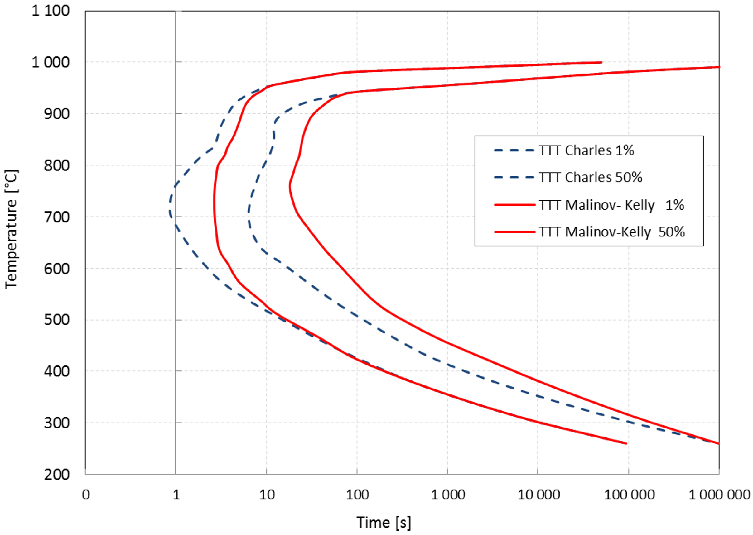
The behavior of the microstructural model described in Section 3 has been tested in simple cases of continuous cooling at constant rates between 10 and 50 K/min. When temperature drops below = 998 °C the formation of the Widmanstätten fraction is calculated according to Equation (17). The evolution of for continuous cooling obtained by Charles et al. [10] have been considered as a reference for the calibration procedure. The same input data used in [10] have been adopted to evaluate the response of the two models. The temperature dependent function used is reported in Table 1 [25]. The TTT curves used are reported in Figure 5 in dashed lines.
The numerical results are reported in Figure 6 where remarkable agreement with the reference model is achieved. Note that the model proposed by Charles et al. takes also into account the formation of grain boundary during transformation and they refer to total alpha fraction as the sum of and . Considering that the amount of phase is typically very low, the contribution of this minor phase has been neglected in this work. Moreover, as typically forms at the beginning of the solid state transformation, the underestimation of total fraction affects only the initial part of the evolution curves.
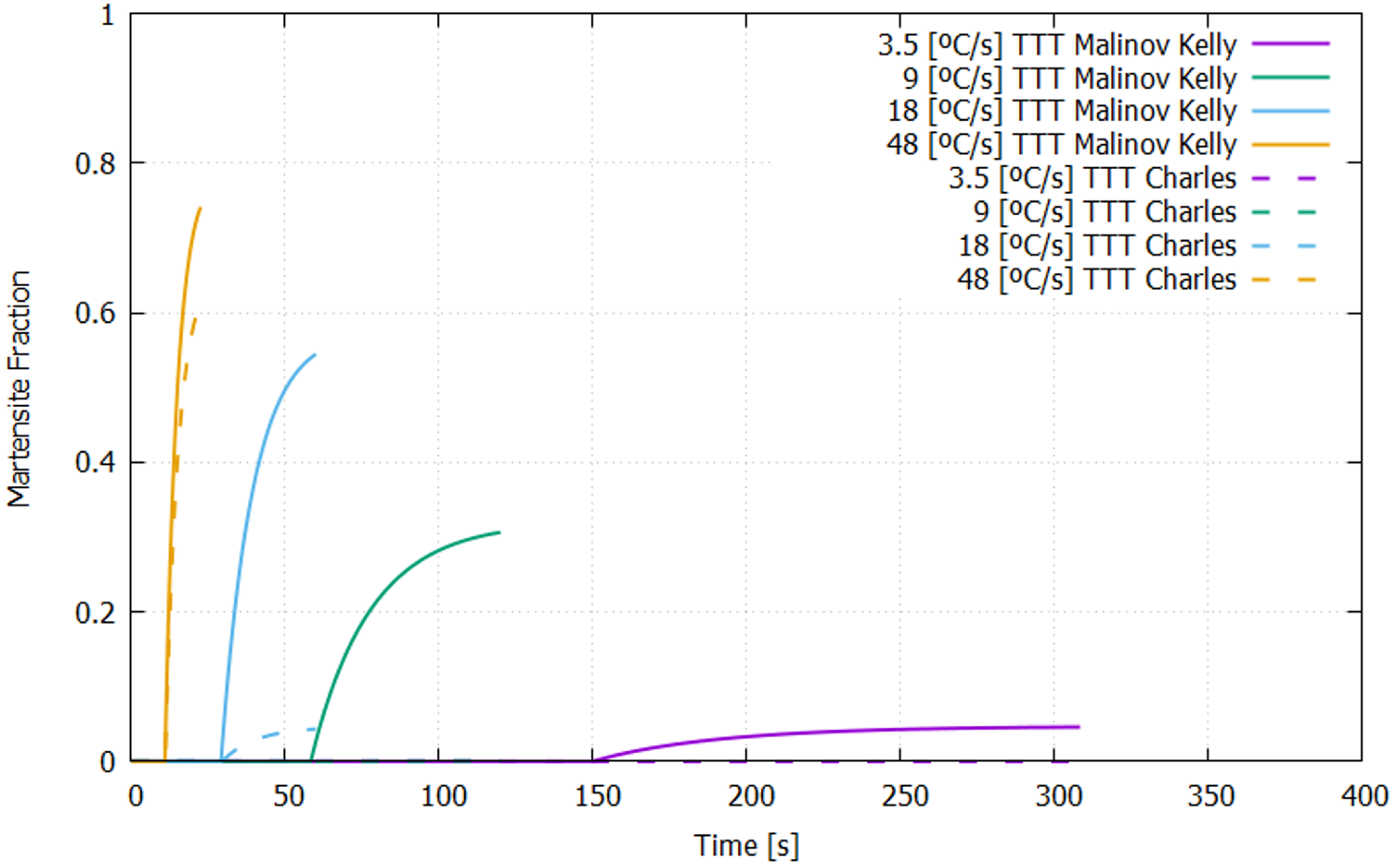
The model has been tested also in case of faster cooling rates allowing for martensite () formation. The computation of martensite evolution begins when the temperature drops below according to the modified Koistinen equation (19). Different values of the parameters (,) are reported in literature ([24,25,28]) and several simulations have been performed varying these 2 parameters which influence the amplitude and the starting point of the transformation, respectively. However, martensite content strongly depends on the amount of residual still available at after the transformation. Martensite fraction evolutions calculated for cooling rates varying between and 48 K/s are reported in Figure 7 assuming = 575 °C and as in [10]. Two different sets of TTT curves have been used for the transformation.
The results reported in dashed lines are obtained using TTT diagrams as proposed by Charles et al. (see Figure 5). Note that in this case only very fast cooling rates (48 K/s) allow for significative martensite formation. For slower cooling rates, this fraction is negligible (less than 5%) in most of the cases. Optical micrographies of Ti6Al4V have been used to evaluate the accuracy of the numerical results obtained. For similar ranges of cooling rates, some qualitative results are found in literature ([16,24]). The experimental results from the two different references present some variability due to the different process conditions. However, these experimental results, reported in Table 2, have been used for a first validation of the numerical model.
The numerical results obtained using the TTT diagrams from Charles et al. show a poor correlation for cooling rates between 9 and 18 K/s. This discordance may be due to a fast formation of , that does not let enough residual for the martensitic transformation.
For this reason, another set of TTT data available in literature has been tested (continuous lines in Figure 5). Observe that there is a great difference between these transformation diagrams. There exists a large number of experimental data performed at high temperatures (750–1000 °C) as those reported by Malinov [26,27], while is more difficult to find a characterization of such curves at lower temperature (e.g., TTT diagrams by Kelly [9]). Combining the TTT data from Malinov and Kelly, the TTT curves shown by continuous line in Figure 5 have been obtained. Using this data the numerical model results in a better agreement for the entire range of cooling rates analyzed, as shown in Figure 7 (continuous lines). The proposed set of TTT diagrams leads to a more gradual transition between fully martensitic and fully Widmanstätten structures and a better overall agreement with the actual microstructures.
4.2. Re-Heating Process and Isothermal Treatment
Several analyses are also performed for isothermal treatments and heating conditions.
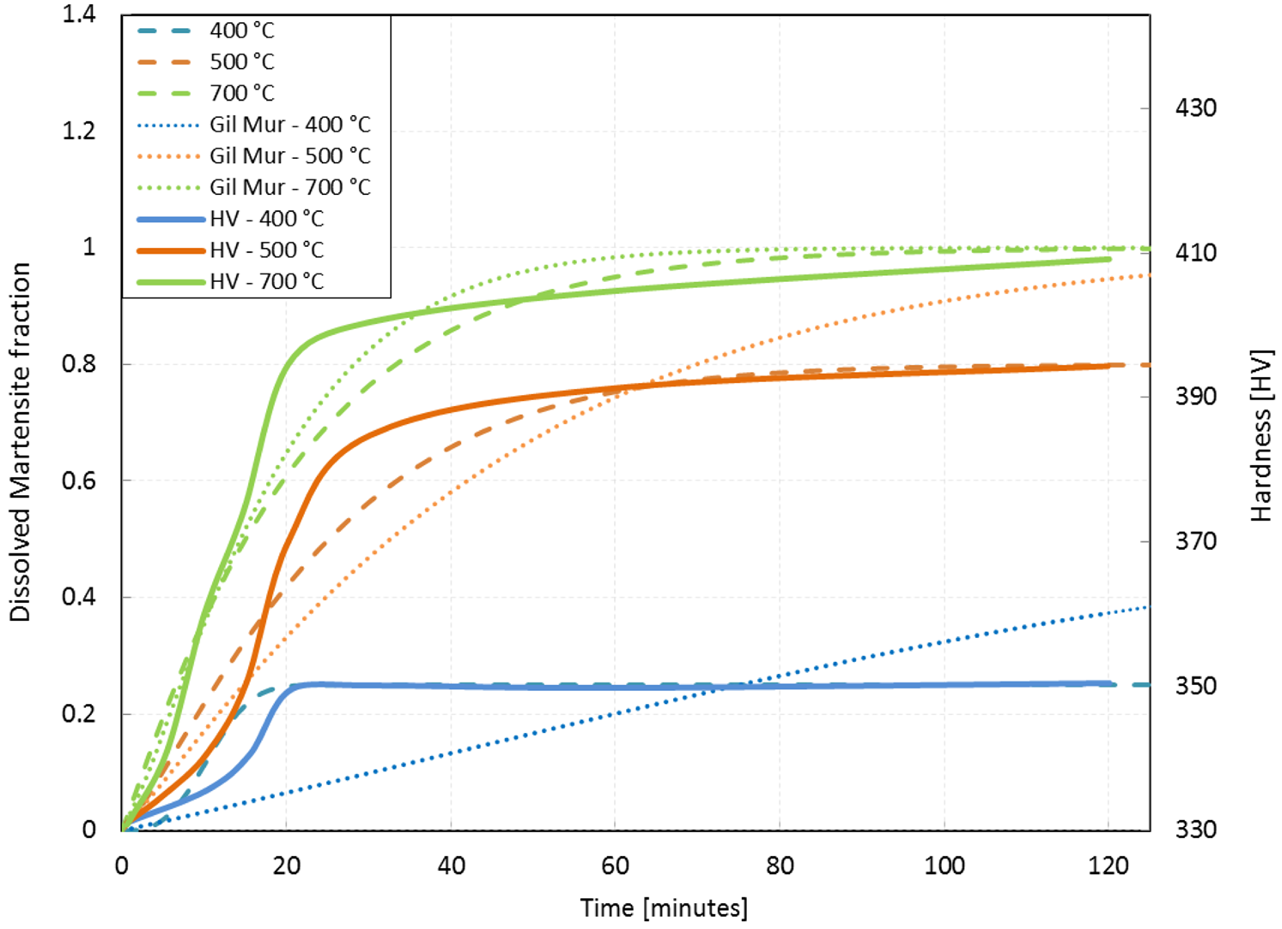
The martensite dissolution at low temperatures has been characterized by the work of Gil Mur [20], where the JMAK parameters k and p that drive the transformation were indirectly obtained from measured hardness of Ti6Al4V samples. For different values of temperature, fully martensitic samples were subjected to isothermal treatments and the resulting Hardness Vickers (HV) was measured at different times of the treatments. For each temperature value, an evolution of HV was found as shown in Figure 8. Note that HV is directly correlated with the martensite content. Hence, the work of Gil Mur establishes a relationship between hardness measurement and the dissolution of the martensite content for different isothermal treatments which can be represented by TTT curves. From the experimental data it can be seen that, at low temperatures, only a small fraction of the total martensite content can be dissolved, even for very long heat treatments. At high temperatures, around 700 °C the martensite dissolution is maximum.
The results of martensite dissolution during isothermal treatments calculated using the traditional JMAK equations as in [20] (dotted lines) and using the model proposed in Section 3.2.3 (dashed lines) are shown in Figure 8. The TTT curves and the function employed in the proposed model are reported in Table 3 and are extracted from Gil Mur’s HV data (see Figure 8), considering martensite dissolution directly proportional to the HV. No martensite dissolution () corresponds to the minimum value of 330 HV. corresponds to a total martensite dissolution and a maximum Hardness of 410 HV. The TTT curves are related to the evolution of the normalized fraction (see Equation (22)). For martensite dissolution has not started. For martensite dissolution has reached the maximum value of . The evolution curves calculated using the proposed model show a remarkable accuracy in the prediction of the actual martensitic dissolution, particularly at low temperatures.
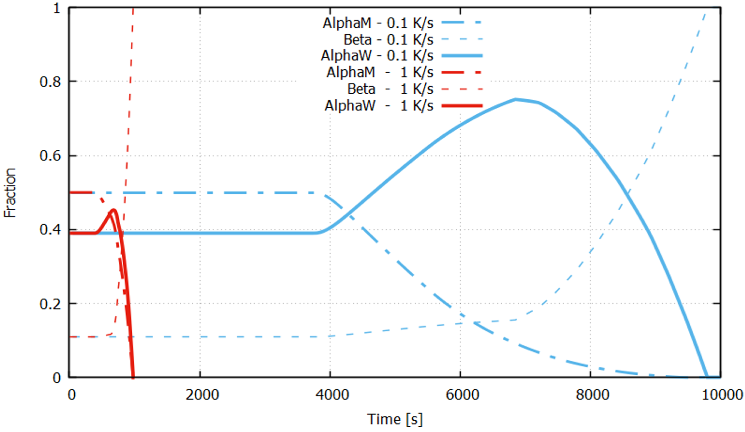
The model has been tested also for continuous heating processes where the dissolution of total into has been modelled according to Equation (25). Function for Ti6Al4V has been used as calibrated by Kelly [9]: () where is the temperature in Kelvin. The fraction is calculated as and is the same input as used for the formation (Table 1). The evolutions of Alpha Widmanstätten, Martensite and Beta computed for continuous heating of and 1 K/s are reported in Figure 9, assuming an initial martensite content of . During the medium-slow heating of K/s, a first growth of and due to the martensite dissolution is clearly visible. In this case, the dissolution of into is almost completed in 40 min in accord with the experimental data of Figure 8. For higher temperatures, the faster transformation of total into begins and also fraction decreases. Note that the martensite dissolution is a slow process if compared with the other transformations. In fact, except for a small initial growth of , the effects of dissolution are not significative for the fastest heating rate (1 K/s). Hence, for medium-fast heating rates the martensite dissolution is almost negligible in comparison with the transformation of total into .
In [11], Fachinotti et al. suggested that martensite dissolution may take place not only during heating but even during slow cooling at temperature above . This may happen when the alloy starts cooling fast at high temperature and then the cooling rate gradually slows down converging to a temperature that allows for martensite dissolution. These cooling conditions are not unusual in AM, because the heat is preserved due the sequence of depositions, especially when back plate heating systems are employed. For these reasons, the model presented in this work can take into account martensite dissolution also during slow cooling. An example of phase fraction evolutions calculated in these conditions is presented in Figure 10. The proposed temperature evolution (dashed line) shows a fast cooling at the beginning that allows for the formation of martensite. Then the cooling continues at temperatures about 500 °C. This slow cooling can be compared to an isothermal treatment. As the alloy remains long time at this medium-high temperature, martensite has time to transform into while cooling.
4.3. AM Processes-Experimental Validation
The microstructural model has been also tested using the thermal cycles obtained during additive manufacturing.
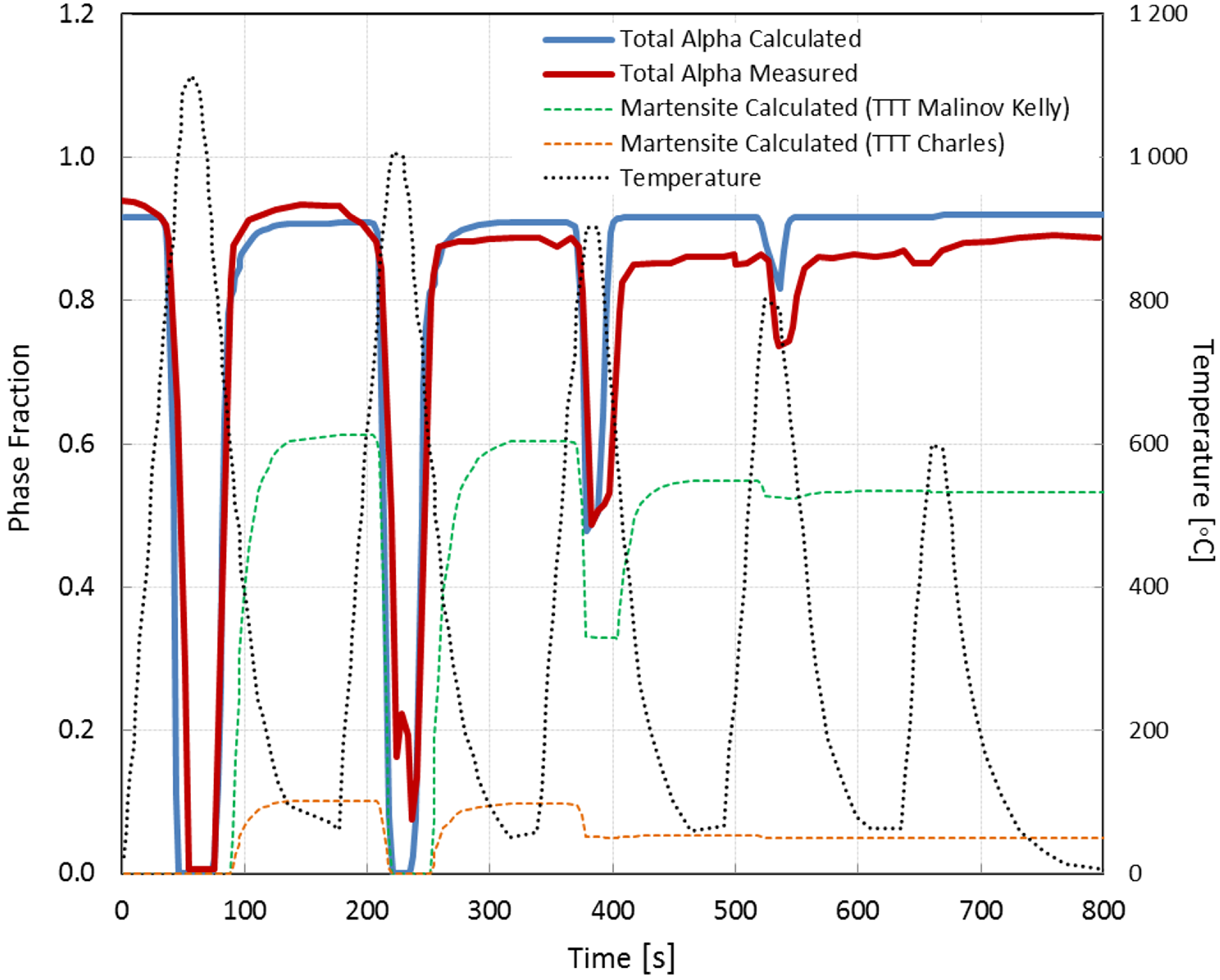
The laser metal deposition process presented by Babu et al. in [29] has been considered as a reference. In his work, Babu measured the evolution of the total alpha phase fraction using X-ray diffraction techniques. These results and the corresponding temperature evolution during the sequential metal depositions are reported in Figure 11. The temperature evolution has been used for the computation of the fractions evolution with the model proposed in Section 3. The calculated evolution of total alpha fraction presented in Figure 11 agrees with the measured values. The evolution of the martensite fraction calculated using reported TTT data is also shown. As expected, the final martensite content obtained with the slower TTT curves from Malinov-Kelly is sensibly higher than that obtained with the TTT curves from Charles et al. Unfortunately, no experimental data of martensite content are available for this test case. Nevertheless, the martensite accumulation induced by the iterative thermal cycles is clearly visible. This phenomenon depends on the different transformation rates of martensite during cooling and heating, respectively. In fact, as martensite formation in cooling is faster than its dissolution in heating, an accumulation is possible during AM thermal cycles.
The experimental data from the work of Xu et al. [30] on Ti6Al4V AM samples have been also considered in order validate the model under different manufacturing conditions. In this case, Ti6Al4V cubes (10 mm side) were produced by SLM (selective laser melting) technology varying different parameters that influence the final content. Two specimen cubes (S3 and S5) fabricated with different energy density have been considered for the validation of the microstructural model. The main process parameters and the microstructures observed at the center of the specimen are reported in Table 4. The different levels of energy density have been obtained by varying the hatch distance. Martensite usually forms during the fast SLM deposition. If the temperatures raise for enough time during the process, can transform into fine lamellar . In these experiments, the base plate was preheated at 200 °C in order to promote martensite dissolution. More details about the process conditions can be found in reference [30].
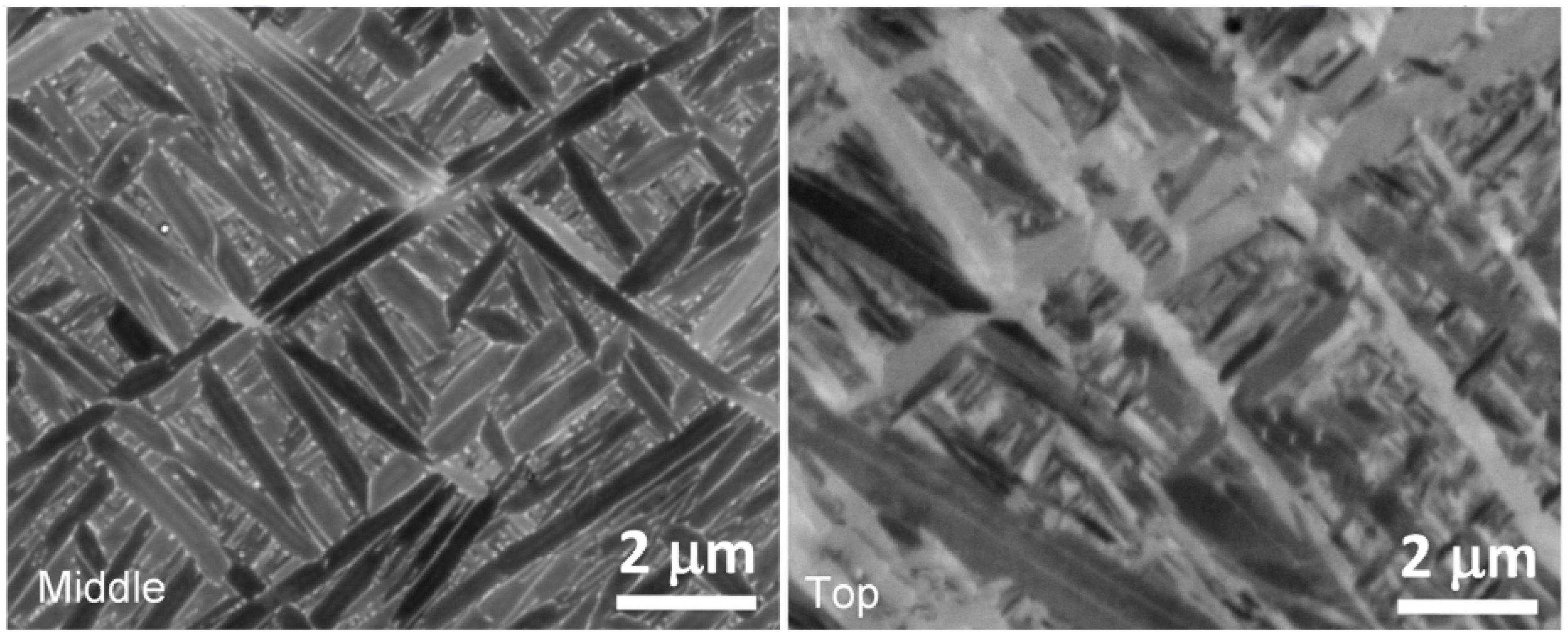
The resulting phase fraction have been evaluated via SEM (scanning electron microscopy) and XRD (X-ray diffraction). Microstructural examination at the center of the cubes shows an high content of in sample S3 due to an almost complete martensite dissolution. On the contrary, the sample S5, fabricated with lower energy density, shows a major content of . The microstructures have been observed also in different parts of the cubes. Scanning electron microscopy (BSE) images of sample S3 from [30] are reported in Figure 12, showing an ultrafine lamellar structure in the middle region and acicular structures in the upper region.
The temperature and the microstructure evolution during the entire fabrication of samples S3 and S4 have been computed using COMET, considering the process parameters reported in [30] (see Table 4). The FE discretization consists of a structured mesh of 25,700 hexahedral elements and 30778 nodes. As regards the microstructural model, the same material data presented in Section 4.1 (TTT diagrams from Malinov and Kelly in Figure 5 for formation and empirical parameters for formation) and Section 4.2 (Kelly function for transformation) have been employed, except for the martensite dissolution. A set of TTT curves for martensite dissolution has been calibrated in order to match the final content of samples S3 and S4. These TTT data are reported in Table 5 and show a faster dissolution in SLM processes, if compared with the data from [20] which refer to heat treatments of samples obtained by casting.
In order to reduce the computational time, the simulation has been performed using a layer by layer metal deposition. As observed in [14], the layer by layer strategy causes the loss of detail in the evaluation of the high temperature peaks during the layer solidification but does not influence the average temperature evolution during the overall SLM process. As the considered solid state transformations take place at medium-low temperatures, the layer by layer strategy does not influence the results of final phase content. In fact, during the process simulation, forms during the cooling of each layer and then starts to dissolve due to heat accumulation in the part.
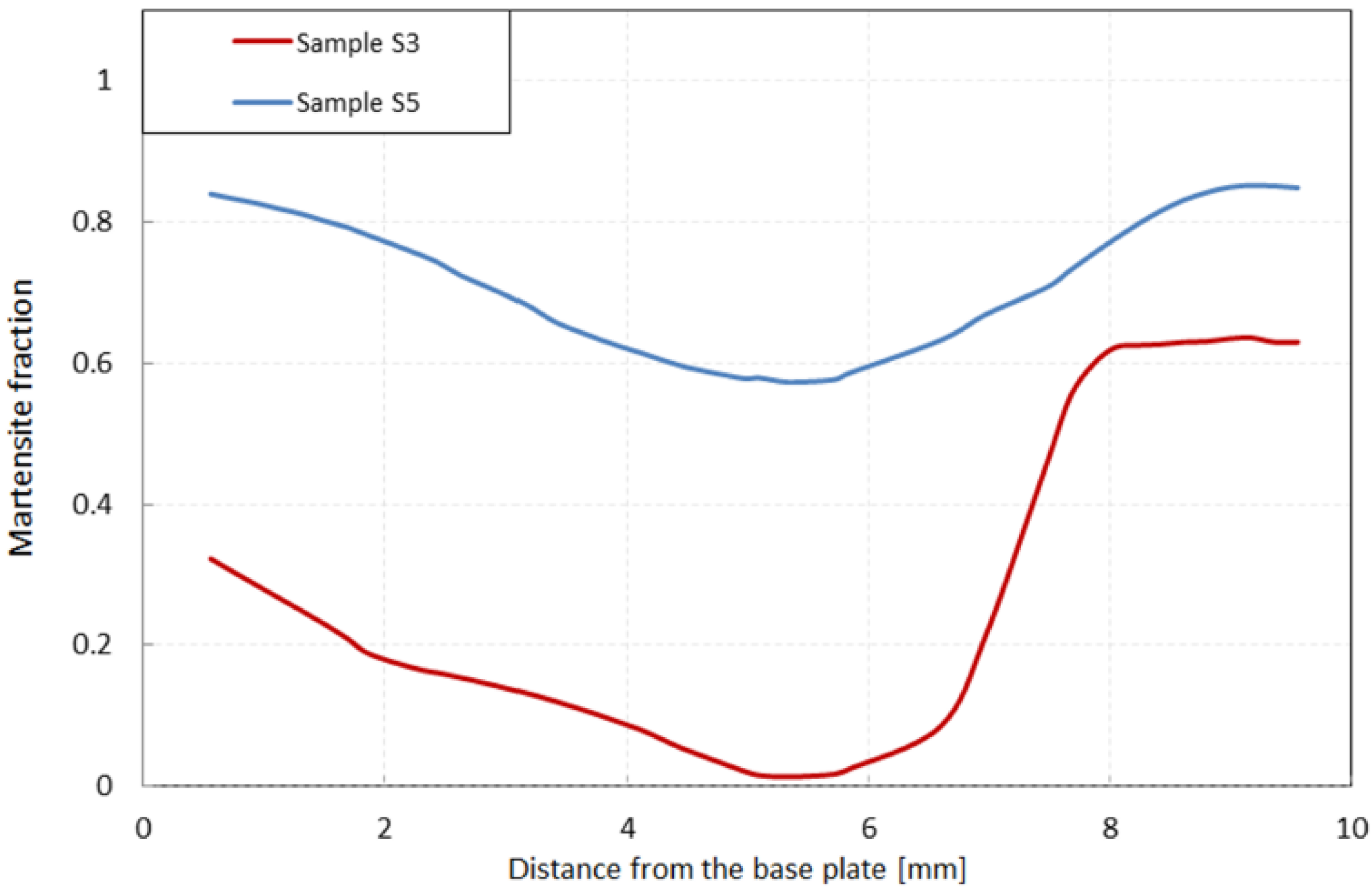
In Figure 13 the calculated final fractions along a vertical line at the center of the cubes are reported. High martensite fractions are obtained at the top of the cubes. This region corresponds to the last deposited layers, where martensite had less time to dissolve due to the lack of successive depositions. These results are totally in line with the microstructure observed by scanning electron microscopy of sample S3 (see Figure 12).
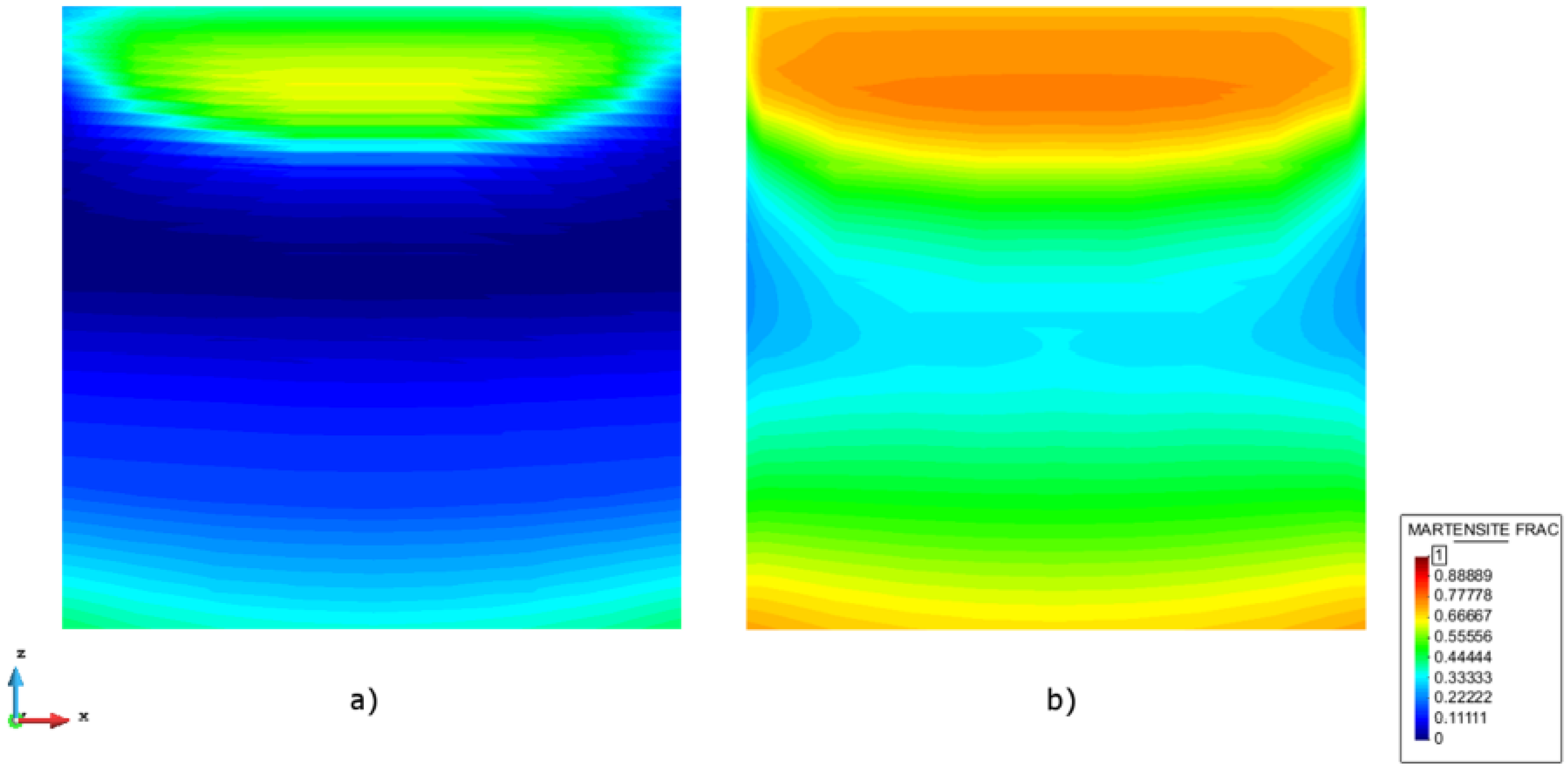
The contour fill of the calculated fraction at the end of the process is reported in Figure 14 for a vertical section xz along the middle plane of the samples (z is the building direction). In the sample S3 fabricated with high energy density, a low martensite content is obtained (Figure 14a). The high temperatures reached during the process allow for an almost complete martensite dissolution at the center of the sample ( = 0.13). In the sample S5 fabricated with lower energy density, a higher content of martensite is obtained (Figure 14b). The lower temperatures obtained during the process do not allow for a total martensite dissolution, leading to a mixed microstructure at the center of the cube ( = 0.57). The calculated fractions at the center of the cubes are in line with the qualitative microstructural evaluation performed via X-ray diffraction and reported in Table 4. These results show the adeguate response of the model to the change of process parameters.
5. Conclusions
Microstructural modeling is necessary to predict material properties in terms of evolution of phases. This is one of the big challenges for the numerical simulation of additive manufacturing processes.
In this paper, a model allowing for the prediction of the microstructure phase evolution of Ti6Al4V alloys in AM processes is presented. The model is specifically designed to deal with AM processes where fast cooling and re-heating cycles occur because: (a) it is able to consider incomplete transformations and varying initial content of phases and (b) it can take into account simultaneous transformations.
The model has been implemented in an in-house FE-based framework for the thermal simulation of AM processes. Sensitivity analysis is carried out to characterize the metallurgical model for different process conditions. Slow rates of martensite dissolution during heating have been appreciated. This behavior, combined with the high speed of martensite formation during cooling leads to martensite accumulation during fast thermal cycles typical of AM processes. Contrarily, depending on the process parameters (i.e., scanning strategy, heat transfer coefficients etc.), high temperature field can develop at some area of the deposited part. These high temperatures allow for complete martensite dissolution, avoiding the need of post-heat treatments. Hence, the thermal and metallurgical simulation of AM can be used to optimize the process parameters and the scanning strategy.
Finally, microstructural measurements from literature of Ti6Al4V samples fabricated by AM process with different manufacturing conditions have been used to validate the model. The model can be enhanced by considering not only phase evolution but also other microstructural features, such as the lath thickness and also size and orientation of grains obtained during solidification.
Author Contributions
E.S., M.C. (Michele Chiumenti) and M.C. (Miguel Cervera) developed the numerical model; E.S. analyzed the data.
Funding
Financial support from the European Union’s Horizon 2020 research and innovation programme under the Marie Skłodowska-Curie Grant Agreement No. 746250, from the European Council-Factories of the Future (FoF) Program under the CAxMan Project-Computer Aided Technologies for Additive Manufacturing-within Horizon 2020 Framework Programme, from the European Council-H2020 MG 2015 SingleStage-A Program under EMUSIC Project-Efficient Manufacturing for Aerospace Components Using Additive Manufacturing, Net Shape HIP and Investment Casting and from the Spanish Government-MINECO-Proyectos de I + D (Excelencia)-DPI2017-85998-P-ADaMANT-Computational Framework for Additive Manufacturing of Titanium Alloy is gratefully acknowledged.
Conflicts of Interest
The authors declare no conflict of interest.
References
- Saboori, A.; Gallo, D.; Biamino, S.; Fino, P.; Lombardi, M. An Overview of Additive Manufacturing of Titanium Components by Directed Energy Deposition: Microstructure and Mechanical Properties. Appl. Sci. 2017, 7, 883. [Google Scholar] [CrossRef]
- Gibson, I.; Rosen, D.; Stucker, B. Additive Manufacturing Technologies; Springer: New York, NY, USA, 2015. [Google Scholar]
- Costa, L.; Vilar, R. Laser powder deposition. Rapid Prototyp. J. 2009, 15, 264–279. [Google Scholar] [CrossRef]
- Selcuk, C. Laser metal deposition for powder metallurgy parts. Powder Metall. 2011, 54, 94–99. [Google Scholar]
- Kar, S.; Searles, T.; Lee, E.; Viswanathan, G.B.; Tiley, J.; Banerjee, R.; Fraser, H.L. Modeling the tensile properties in β processed α/β Ti alloys. Metall. Mater. Trans. A 2006, 37, 559–566. [Google Scholar] [CrossRef]
- Avrami, M. Kinetics of phase change: III. Granulation, phase change, and microstructure. J. Chem. Phys. 1941, 9, 177–184. [Google Scholar] [CrossRef]
- Cahn, J. Transformation kinetics during continuous cooling. Acta Metall. 1956, 4, 572–575. [Google Scholar] [CrossRef]
- Koistinen, D.P.; Marburger, R.E. A general equation prescribing the extent of the austenite-martensite transformation in pure iron-carbon alloys and plain carbon steels. Acta Metall. 1959, 7, 59–60. [Google Scholar] [CrossRef]
- Kelly, S. Thermal and Microstructure Modeling of Metal Deposition Processes with Application to Ti6Al4V. Ph.D. Thesis, Faculty of Virginia, Polytechnic Institute and State University, Blacksburg, VA, USA, 2004. [Google Scholar]
- Charles Murgau, C.; Pederson, R.; Lindgren, L. A model for Ti-6Al-4V microstructure evolution for arbitrary temperature changes. Model. Simul. Mater. Sci. Eng. 2012, 20, 055006. [Google Scholar] [CrossRef]
- Fachinotti, V.; Cardona, A.; Baufeld, B.; Van der Biest, O. Evolution of microstructure during shaped metal deposition. Mecánica Comput. 2010, 29, 4927–4934. [Google Scholar]
- Chiumenti, M.; Cervera, M.; Salmi, A.; Agelet de Saracibar, C.; Dialami, N.; Matsui, K. Finite element modeling of multi-pass welding and shaped metal deposition processes. Comput. Methods Appl. Mech. Eng. 2010, 199, 2343–2359. [Google Scholar] [CrossRef]
- Agelet de Saracibar, C.; Lundbäck, A.; Chiumenti, M.; Cervera, M. Shaped Metal Deposition Processes. In Encyclopedia of Thermal Stresses; Hetnarski, R.B., Ed.; Springer: Dordrecht, The Netherlands; Heidelberg, Germany; New York, NY, USA; London, UK, 2014; pp. 4346–4355. [Google Scholar]
- Chiumenti, M.; Neiva, E.; Salsi, E.; Cervera, M.; Badia, S.; Moya, J.; Chen, Z.; Lee, C.; Davies, C. Numerical Modelling and Experimental Validation in Selective Laser Melting. Addit. Manuf. 2017, 18, 171–185. [Google Scholar] [CrossRef]
- Charles Murgau, C. Microstructure Model for Ti-6Al-4V Used in Simulation of Additive Manufacturing. Ph.D. Thesis, University of Luleå, Luleå, Sweden, 2016. [Google Scholar]
- Sieniawski, J.; Ziaja, W.; Kubiak, K.; Motyka, M. Microstructure and Mechanical Properties of High Strength Two-Phase Titanium Alloys. In Titanium Alloys—Advances in Properties Control; Sieniawski, J., Ed.; InTech: Rijeka, Croatia, 2013. [Google Scholar] [Green Version]
- Donachie, M. Titanium: A Technical Guide; ASM International Materials: Park, OH, USA, 2000. [Google Scholar]
- Porter, D.A.; Easterling, K.E. Phase Transformations in Metals and Alloys, 2nd ed.; Chapman & Hall: London, UK, 1992. [Google Scholar]
- Gil, F.J.; Ginebra, M.P.; Manero, J.M.; Planell, J.A. Formation of alpha-Widmanstatten structure: Effects of grain size and cooling rate on theWidmanstatten morphologies and on the mechanical properties in Ti6Al4V alloy. J. Alloy. Compd. 2001, 329, 142–152. [Google Scholar] [CrossRef]
- Gil Mur, F.X.; Rodríguez, F.D.; Planell, J.A. Influence of tempering temperature and time on the alpha prime Ti-6Al-4V martensite. J. Alloy. Compd. 1996, 234, 287–289. [Google Scholar] [CrossRef]
- Charles Murgau, C.; Jarvstrat, N. Modelling Ti-6Al-4V microstructure by evolution laws implemented as finite element subroutine. In Proceedings of the 8th International Conference on Trends in Welding Research, Pine Mountain, GA, USA, 1–6 June 2008. [Google Scholar]
- Johnson, W.; Mehl, R. Reaction Kinetics in processes of nucleation and growth. Trans. Am. Inst. Min. Metall. Eng. 1939, 135, 416–458. [Google Scholar]
- Kolmogorov, A. Statistical theory of crystallization of metals (in Russian). Izv. Akad. Nauk SSSR Ser. Math. 1937, 1, 355–359. [Google Scholar]
- Ahmed, T.; Rack, H.J. Phase transformations during cooling in α + β titanium alloys. Mater. Sci. Eng. A 1998, 243, 206–211. [Google Scholar] [CrossRef]
- Castro, R.; Seraphin, L. Contribution in the metallographic and structural study of the alloy of titanium Ti4Al6V. Mem. Sci. Rev. Metall. 1966, 63, 1025–1058. [Google Scholar]
- Malinov, S.; Guo, Z.; Sha, W.; Wilson, A. Differential scanning calorimetry study and computer modeling of β to α phase transformation in a Ti-6Al-4V alloy. Metall. Mater. Trans. A 2001, 32, 879–887. [Google Scholar] [CrossRef]
- Malinov, S.; Markovsky, P.; Sha, W.; Guo, Z. Resistivity study and computer modelling of the isothermal transformation kinetics of Ti–6Al–4V and Ti-6Al-2Sn-4Zr-2Mo-0.08Si alloys. J. Alloy. Compd. 2001, 314, 181–192. [Google Scholar] [CrossRef]
- Elmer, J.W.; Palmer, T.A.; Babu, S.S.; Zhang, W.; DebRoy, T. In-situ observations of phase transformations in the fusion zone of Ti-6Al-4V alloy transient welds using synchrotron radiation. In Mathematical Modelling of Weld Phenomena; Cerjak, H., Ed.; Verlag der Technische Universitat Graz: Graz, Austria, 2005; Volume 7. [Google Scholar]
- Babu, S.S.; Kelly, S.M.; Specht, E.D.; Palmer, T.A.; Elmer, J.W. Measurement of phase transformation kinetics during repeated thermal cycling of Ti-6Al-4V using time-resolved X-ray diffraction. In Proceedings of the International Conference on Solid-Solid Phase Transformations in Inorganic Materials, Phoenix, AZ, USA, 29 May–3 June 2005. [Google Scholar]
- Xu, W.; Brandt, M.; Sun, S.; Elambasseril, J.; Liu, Q.; Latham, K.; Xia, K.; Quian, M. Additive manufacturing of strong and ductile Ti-6Al-4V by selective laser melting via in situ martensite decomposition. Acta Mater. 2015, 85, 74–84. [Google Scholar] [CrossRef]
Figure 1.
Ti6Al4V microstructures at room temperature. (a) Widmanstätten alpha [15]; (b) Grain boundary alpha [15]; (c) Martensite [16].

Figure 2.
Example of Additivity Rule for 2 isothermal steps. Definition of the evolution of phase fraction X as the sum of the contributions of different sets of k,p parameters extracted from the TTT (Temperature-Time-Transformation) curves.
Figure 2.
Example of Additivity Rule for 2 isothermal steps. Definition of the evolution of phase fraction X as the sum of the contributions of different sets of k,p parameters extracted from the TTT (Temperature-Time-Transformation) curves.
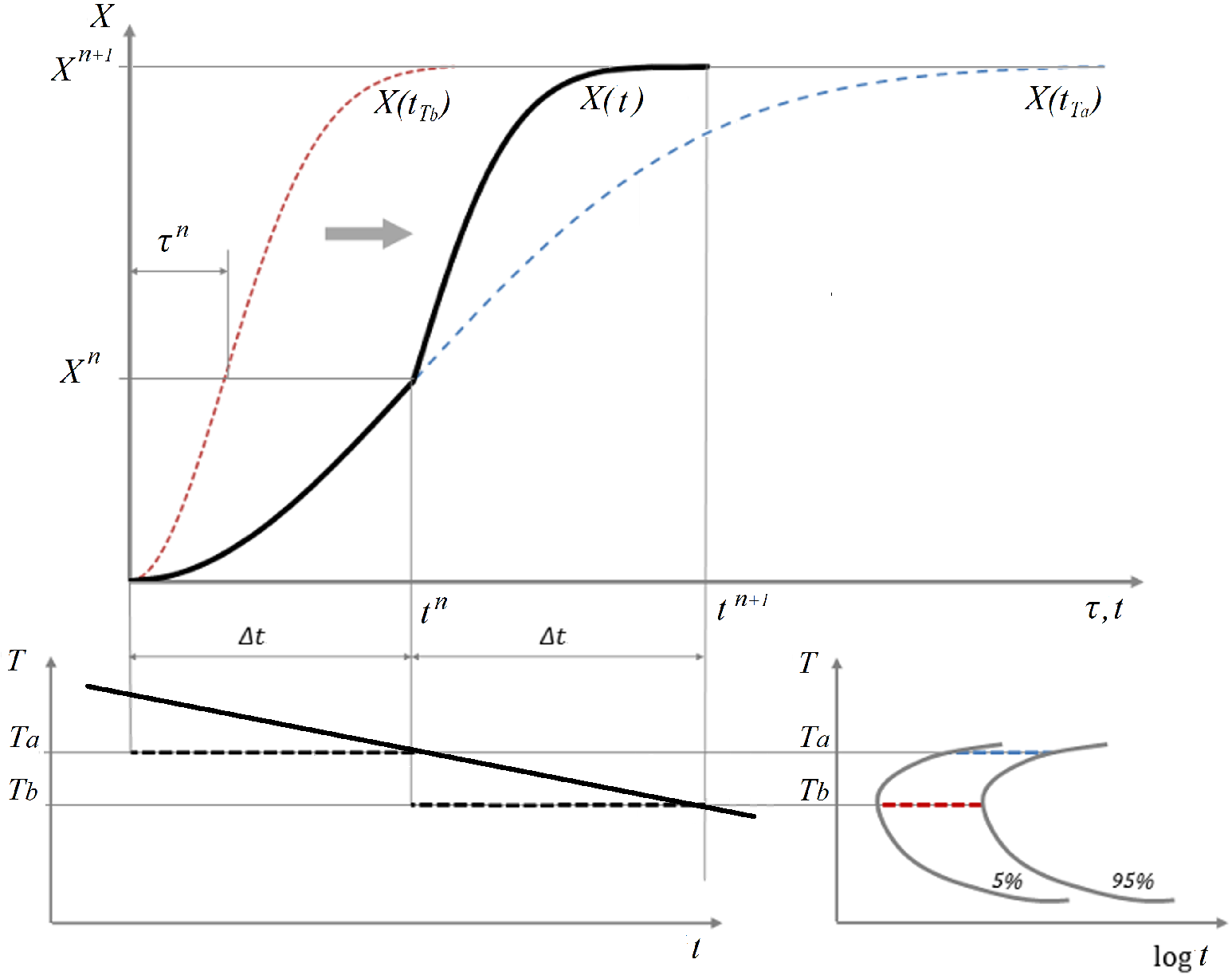
Figure 3.
Schematic representation of the 4 main solid state transformation considered in the proposed model.
Figure 3.
Schematic representation of the 4 main solid state transformation considered in the proposed model.
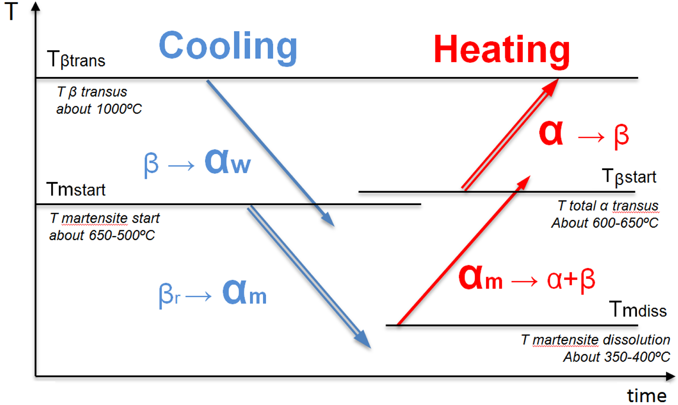
Figure 4.
Flowchart for microstructure model implementation.

Figure 5.
TTT-diagrams for Ti6Al4V: proposed from Charles et al. in [10] (dashed line) and a mix of Malinov’s [26,27] and Kelly’s [9] data (continuous line).

Figure 6.
Alpha phase evolution calculated for different cooling rates. Comparison with numerical results from Charles et al. model [10] (same TTT material input).
Figure 6.
Alpha phase evolution calculated for different cooling rates. Comparison with numerical results from Charles et al. model [10] (same TTT material input).
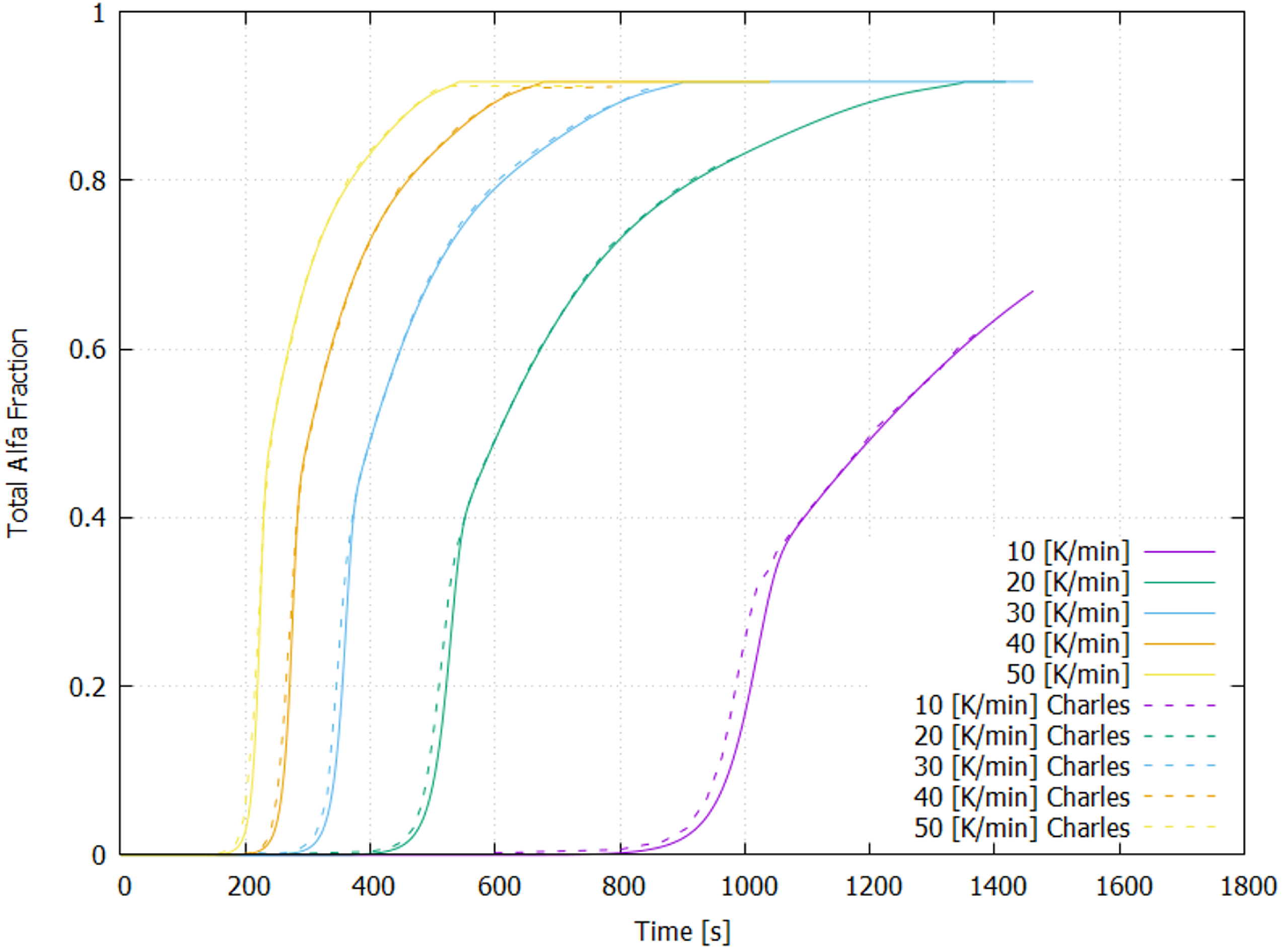
Figure 7.
Martensite fraction evolution during continuous coolings. Comparison between results obtained with TTT proposed by Charles et al. [10] and with TTT obtained by a mix of Malinov’s [26,27] and Kelly’s [9] data.

Figure 8.
Experimental data of hardness evolution during isothermal treatments by Gil Mur [20] (continuous line) and fraction evolution of dissolved martensite during isothermal treatments calculated using the present model (dashed line) and using JMAK equations with parameters k, p reported by Gil Mur.

Figure 9.
Calculated fraction evolution of Alpha Widmanstatten, Martensite and Beta during continuous heating (0.1–1 K/s).
Figure 9.
Calculated fraction evolution of Alpha Widmanstatten, Martensite and Beta during continuous heating (0.1–1 K/s).

Figure 10.
Calculated fraction evolution of Alpha Widmanstatten, Martensite and Beta during a gradual slowing cooling rate.
Figure 10.
Calculated fraction evolution of Alpha Widmanstatten, Martensite and Beta during a gradual slowing cooling rate.
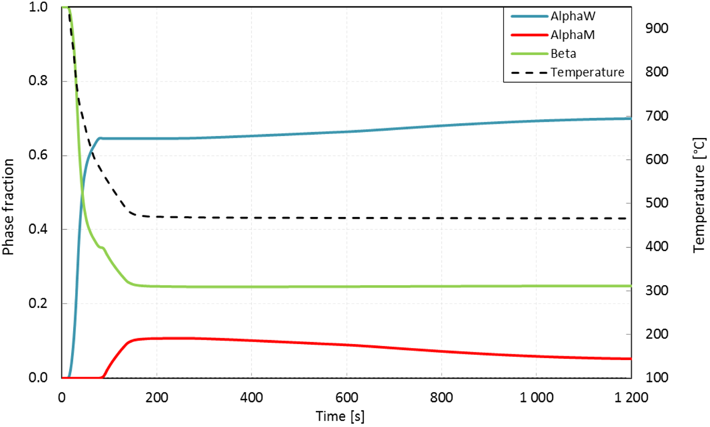
Figure 11.
Successive cycles of metal deposition. Evolution of temperature and of total alpha fraction measured by Babu [29]. Evolution of total alpha and martensite fractions calculated with the present model.
Figure 11.
Successive cycles of metal deposition. Evolution of temperature and of total alpha fraction measured by Babu [29]. Evolution of total alpha and martensite fractions calculated with the present model.

Figure 12.
Scanning electron microscopy (BSE) of SLM fabricated sample S3 in the middle and top regions [30].
Figure 12.
Scanning electron microscopy (BSE) of SLM fabricated sample S3 in the middle and top regions [30].

Figure 13.
Calculated final fraction along a vertical line at the center of the samples S3 and S5.

Figure 14.
Contour fill of calculated final fraction in a vertical section xz along the middle plane of the samples S3 (a) and S5 (b).
Figure 14.
Contour fill of calculated final fraction in a vertical section xz along the middle plane of the samples S3 (a) and S5 (b).

Table 1.
Alpha fraction at equilibrium at different temperatures: maximum final fraction of alpha phase that can form at equilibrium at temperature T according with the phase diagram of the alloy.
Table 1.
Alpha fraction at equilibrium at different temperatures: maximum final fraction of alpha phase that can form at equilibrium at temperature T according with the phase diagram of the alloy.
| Temperature (°C) | Alpha Fraction at Equilibrium αeq |
|---|---|
| 1000 | |
| 988 | |
| 967 | |
| 940 | |
| 913 | 0.39 |
| 898 | |
| 863 | |
| 829 | |
| 799 | |
| 767 | |
| 742 | |
| 710 | |
| 684 | |
| 667 | |
| 650 |
Table 2.
Martensite content at the end of continuous coolings. Comparison between observed microstructures in literature and results obtained with different TTT data inputs.
Table 2.
Martensite content at the end of continuous coolings. Comparison between observed microstructures in literature and results obtained with different TTT data inputs.
| Cooling Rate [K/s] | Observed Microstructures | Calculated αm Martensite Final Fraction | ||
|---|---|---|---|---|
| Ahmed et al. [24] | Sieniawski et al. [16] | Charles et al. TTT | Malinov and Kelly TTT | |
| 3.5 | (trace) | (trace) | 0.0001% | 3% |
| 9 | 0.04% | 30% | ||
| 18 | (trace) | 4% | 57% | |
| 48 | 61% | 77% | ||
Table 3.
Dissolved martensite fraction at equilibrium and initial and final times ti(T), tf(T) of martensite dissolution with initial and final normalized fractions: Xi = 0.3, Xf = 0.9.
Table 3.
Dissolved martensite fraction at equilibrium and initial and final times ti(T), tf(T) of martensite dissolution with initial and final normalized fractions: Xi = 0.3, Xf = 0.9.
| Temperature (°C) | [s] | [s] | |
|---|---|---|---|
| 320 | 0 | ||
| 400 | 500 | 1200 | |
| 500 | 520 | 3600 | |
| 700 | 1 | 450 | 3000 |
Table 4.
Process parameters of the Ti6Al4V cubes S3 and S5 fabricated by SLM in [30] and final phase fraction observed via XRD at the center of the cubes. (P laser power, t layer thickness, v scanning velocity, h hatch spacing, E energy density).
Table 4.
Process parameters of the Ti6Al4V cubes S3 and S5 fabricated by SLM in [30] and final phase fraction observed via XRD at the center of the cubes. (P laser power, t layer thickness, v scanning velocity, h hatch spacing, E energy density).
| Sample | P (W) | t (μm) | v (mm s−1) | h (mm) | E (J mm−3) | Measured Phase Fractions | Calculated αm |
|---|---|---|---|---|---|---|---|
| 375 | 60 | 1029 | 0.12 | 50.62 | 0.13 | ||
| 375 | 60 | 1029 | 0.18 | 33.74 | and | 0.57 |
Table 5.
Dissolved martensite fraction at equilibrium and initial and final times ti(T), tf(T) of martensite dissolution with initial and final normalized fractions: Xi = 0.3, Xf = 0.9. Data calibrated for the simulation of SLM production of samples S3 and S5.
Table 5.
Dissolved martensite fraction at equilibrium and initial and final times ti(T), tf(T) of martensite dissolution with initial and final normalized fractions: Xi = 0.3, Xf = 0.9. Data calibrated for the simulation of SLM production of samples S3 and S5.
| Temperature (°C) | (s) | (s) | |
|---|---|---|---|
| 320 | 0 | ||
| 400 | 300 | 800 | |
| 500 | 250 | 300 | |
| 700 | 1 | 30 | 60 |
© 2018 by the authors. Licensee MDPI, Basel, Switzerland. This article is an open access article distributed under the terms and conditions of the Creative Commons Attribution (CC BY) license (http://creativecommons.org/licenses/by/4.0/).
Share and Cite
MDPI and ACS Style
Salsi, E.; Chiumenti, M.; Cervera, M. Modeling of Microstructure Evolution of Ti6Al4V for Additive Manufacturing. Metals 2018, 8, 633. https://doi.org/10.3390/met8080633
AMA Style
Salsi E, Chiumenti M, Cervera M. Modeling of Microstructure Evolution of Ti6Al4V for Additive Manufacturing. Metals. 2018; 8(8):633. https://doi.org/10.3390/met8080633
Chicago/Turabian StyleSalsi, Emilio, Michele Chiumenti, and Miguel Cervera. 2018. "Modeling of Microstructure Evolution of Ti6Al4V for Additive Manufacturing" Metals 8, no. 8: 633. https://doi.org/10.3390/met8080633
Note that from the first issue of 2016, this journal uses article numbers instead of page numbers. See further details here.