Fatigue Strength Assessment of Welded Mild Steel Joints Containing Bulk Imperfections


1
Christian Doppler Laboratory for Manufacturing Process based Component Design, Chair of Mechanical Engineering, Montanuniversität Leoben, 8700 Leoben, Austria
2
Kyushu University, 819-0395 Fukuoka, Japan
3
Fraunhofer Institute for Mechanics of Materials IWM, 79108 Freiburg, Germany
4
Department of Applied Mechanics, School of Engineering, Aalto University, 02150 Espoo, Finland
*
Author to whom correspondence should be addressed.
Metals 2018, 8(5), 306; https://doi.org/10.3390/met8050306
Submission received: 29 March 2018
/
Revised: 20 April 2018
/
Accepted: 23 April 2018
/
Published: 29 April 2018
(This article belongs to the Special Issue Fatigue and Wear for Steels)
Abstract
:This work investigates the effect of gas pores, as bulk imperfections, on the fatigue strength of welded mild steel joints. Two test series containing different butt joint geometries and weld process parameters are included in order to achieve two variable types of pore sizes. Based on the √area-parameter by Murakami, the test series can be grouped into imperfections exhibiting √area < 1000 µm and √area > 1000 µm. Fatigue tests at a load stress ratio of R = 0.1 are performed, which act as comparison for the subsequent fatigue estimation. To assess the fatigue resistance, the approaches by Murakami, De Kazinczy, and Mitchell are utilized, which highlight certain differences in the applicability depending on the imperfection size. It is found that, on one hand, Murakami’s approach is well suitable for both small and large gas pores depending on the applied model parameters. On the other hand, the fatigue concepts by De Kazinczy and Mitchell are preferably practicable for large defects with √area > 1000 µm. In addition, the method by Mitchell incorporates the stress concentration factor of the imperfection, which can be numerically computed considering the size, shape, and location of the gas pore, as presented in this paper.
1. Introduction
Fatigue strength of welded joints is primarily affected by geometrical parameters, such as the weld toe [1] or root [2] condition, as well as local manufacturing process-dependent characteristics like the effective residual stress state [3], microstructure [4], and hardness condition [5]. Recently, an update of the recommendations for fatigue design of welded joints and components by the International Institute of Welding (IIW) was published [6], which provides a guideline to assess the fatigue strength of steel and aluminum welds based on global and local approaches [7]. Postulating good workmanship weld quality, most of the surface fatigue cracks originate at the weld toe in case of fillet welds, which was also investigated within prior studies for butt joints [8], T-joints, and longitudinal stiffeners [9]. However, the weld quality generally affects the fatigue strength of welded joints, e.g., presented for fillet welds in [10]. Especially for high-strength steels, crack-like flaws, such as undercuts [11], majorly reduce the fatigue resistance [12]. Post-weld improvement techniques [13], like the high-frequency mechanical impact treatment [14,15], are capable to increase the fatigue life of welded structures even in case of small pre-existing surface flaws [16].
Besides these local influences, additionally, global parameters like distortion [17] need to be incorporated within the fatigue assessment to holistically evaluate the fatigue life of complex weld structures. In order to cover all these effects, a weld quality criteria-based fatigue assessment is developed [18], which is additionally published as IIW-guideline [19]. This paper deals with the effect of internal bulk imperfections, in particular gas pores, on the fatigue strength of welded mild steel joints. Especially for very high-cycle fatigue regimes (VHCF), e.g., in the giga-cycle region, defects [20] and further microstructural properties [21,22] affect fatigue crack initiation [23]. An overview of failure mechanisms for metallic alloys is provided in [24]; thereby, porosity acts as one major cause for fatigue crack initiation especially for cast materials and weldments. In [25,26], the significant impact of porosity on the fatigue behavior of welded aluminum alloys is presented. The experimental results of welded Al-Zn-Mg samples in [25] reveal that an increase of the maximum gas pore diameter from dmax = 0.06 mm to 0.72 mm leads to an decrease of the fatigue strength at ten million load-cycles by about 30%. Another study [27] investigates the influence of porosity on the fatigue crack growth behavior of Ti–6Al–4V laser welds. Thereby, it is concluded that the porous weld shows a serration on the crack growth curve and exhibits similar crack growth characteristics as the defect free one. However, only a comparably minor number of documented results focusing on the effect of internal gas porosity on the fatigue strength of welded joints are provided in literature. Therefore, this paper scientifically contributes to the fatigue assessment of welded mild steel joints containing bulk imperfections in order to enhance this field of research. Summarized, this paper includes the following topics based on experimental and analytical/numerical investigations:
- Manufacturing of different mild steel butt joints exhibiting gas pores as representative imperfections with different sizes, shapes, and locations.
- Characterization of local properties, fatigue testing, and fracture surface analysis to investigate the relationship between material condition, defect size, and strength.
- Application of different fatigue models to evaluate the practicability of these concepts in order to assess the fatigue strength of imperfected mild steel weld joints.
2. Materials and Methods
2.1. Materials and Test Series
Within this work, mild steel S355 butt joint specimens are manufactured in two different conditions in order to ensure varying imperfection sizes, shapes, and locations. At first, butt joints with a sheet thickness of t = 16 mm are gas metal arc welded (GMAW) with two weld passes, one bottom (root) and one top layer. This leads to comparably minor gas pores or imperfections, which are therefore denoted as √area < 1000 µm, whereat three specimens are tested. At second, ten butt joints with a sheet thickness of t = 10 mm are manufactured by three-pass GMAW only welded from the top side, featuring comparably larger gas pores, which are therefore denoted as √area > 1000 µm. An overview of the investigated test series is provided in Table 1, covering also details about the nominal cross section in terms of width w and thickness t of the testing area.
Table 2 presents the chemical compositions in weight % of the mild steel S355 base material, which is utilized in rolled and normalized condition within this study.
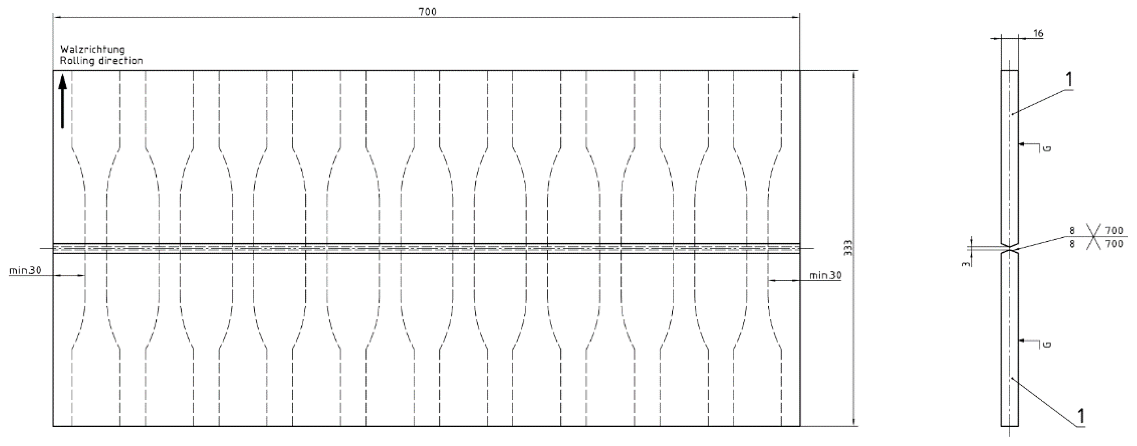
Figure 1 depicts the weld array and the specimen geometry for the test series √area < 1000 µm. The weld array for √area > 1000 µm is basically similar; however, weld preparation and process parameters are different to ensure larger imperfections after welding. Due to the increase of the gas pores, the cross-section is additionally enlarged for the samples of test series √area > 1000 µm to ensure comparable testing conditions. Further details on the specimen geometry, weld preparation, and process parameters are given in [28] for √area < 1000 µm, and in [29,30] for √area > 1000 µm.
2.2. Fatigue Assessment Methods
In [31,32,33], it is illustrated that the square root of the defect area perpendicular to the maximum principal stress direction, denoted as √area-parameter, acts as engineering-feasible value for a defect-size-based fatigue assessment. In [31], it is shown that the fracture mechanical threshold ΔKth in MPa √m at a stress ratio of R = −1 can be estimated based on the material’s Vicker’s hardness HV and the √area-value in µm of the interior defect; see Equation (1).
In [33] it is observed that a slope of 1/3 with m = 3 fits well with experimental data incorporating steels with different base material strengths. Based on this relationship, Murakami [33] introduced a fatigue model, which assesses the mean fatigue strength for internal inclusions; see Equation (2). The approach estimates the high-cycle fatigue resistance σf at a stress ratio of R = −1 for a defined number of ten million load-cycles utilizing a slope of 1/6 with m = 3 for defect sizes with √area < 1000 µm.
Due to the thermo-mechanical manufacturing process, welded joints typically contain residual stresses, which may significantly influence the fatigue strength [34]. In engineering approaches, such residual stresses can be accounted as mean stresses [35] modifying the local-effective stress ratio Reff. In [33], the mean stress correction factor fmean is introduced to estimate the fatigue resistance at varying mean stress states, see Equation (3). This factor is additionally applied for all fatigue models in this work to consider local R-ratios different to R = −1.
Thereby, the stress ratio R can be replaced by the effective stress ratio Reff, which includes the local load stress dependent values σmin and σmax as well as the residual stress σres, see Equation (4).
A recent study in [36] for welded mild and high-strength steel joints shows that the parameter Reff has a remarkable influence on the fatigue strength, especially in the high-cycle fatigue regime, and hence, the local mean stress state needs to be assessed properly within the fatigue assessment.
In [37,38] an overview about fatigue models for a defect tolerant design is given. Due to the basically limited validity of the concept by Murakami for only comparably small defect sizes with √area < 1000 µm, another fatigue approach by De Kazinczy [39], which is generally applicable for larger imperfections exhibiting a value of √area > 1000 µm, is introduced; see Equation (5).
Herein, the utilized defect parameter √d is the diameter of the smallest circle enclosing the imperfection. In [38], it is stated that the value k acts as a constant representing the defect geometry, which exhibits a value of k = 1130 mm1/2MN/m2 for surface micro-shrinkage cavities according to [39]. To transfer this constant to internal bulk defects, an additional consideration of the fracture mechanical geometry factor Y = 2/π for internal round inclusions based on the suggestion in [40] is utilized. The local alternating fatigue strength for a material without imperfections σf0 depends on the local hardness condition and can be estimated by σf0 = 1.6 HV [33,41]. Similarly, the local yield strength σy can be estimated by σy = −90.7 + 2.876 HV according to [42]. In addition to the aforedescribed methods, the concept by Mitchell [43] considers the stress concentration factor Kt at large imperfections for the assessment of the alternating fatigue strength; see Equation (6).
Herein, the material-dependent factor A is evaluated on the basis of the ultimate strength σu, see [43]. According to [42], σu can be estimated by σu = −99.8 + 3.734 HV. The value ρ equals the notch radius of the imperfection. In [44], analytical and numerical computations to evaluate the stress concentration at internal voids are presented. It is shown that for a spherical imperfection, the stress concentration factor Kt can be calculated according to Equation (7) considering the Poisson’s ratio ν of the material. Further details to the analytical evaluation of stress concentration coefficients for internal welding defects are provided in [45].
3. Results
Firstly, this section presents the results of the evaluated local properties and the fatigue tests including a fracture surface analysis. Secondly, the application of the previously described fatigue models is illustrated, showing the accuracy of each approach to assess the experimentally evaluated fatigue strength. A final discussion and comparison of the employed methods is given in Section 4.
3.1. Evaluation of Local Properties and Fatigue Behaviour
3.1.1. Hardness and Residual Stress Condition
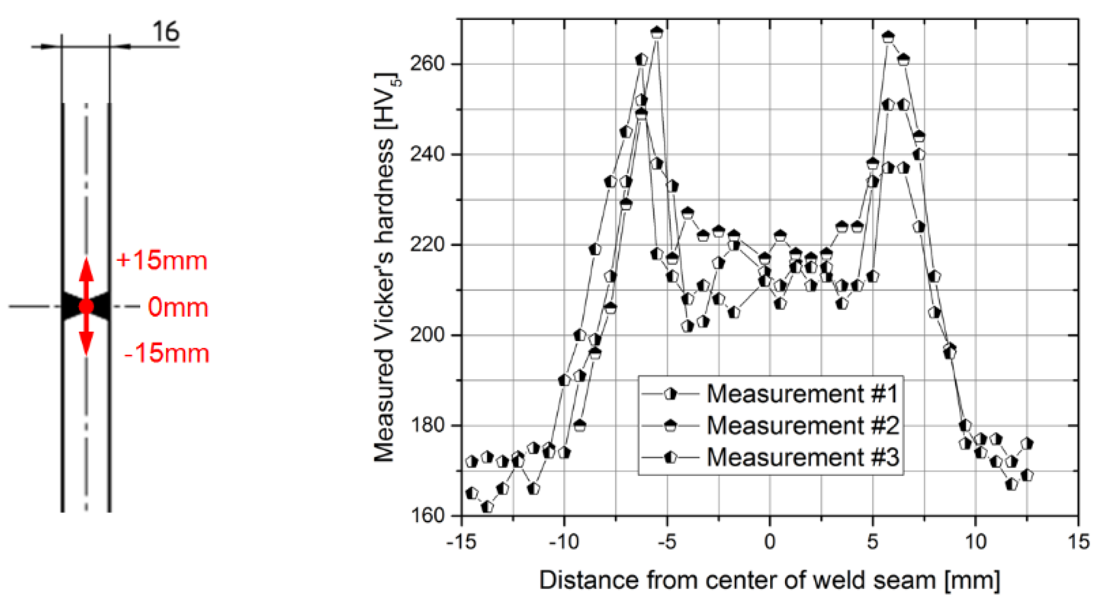
As aforementioned, the fatigue models by Murakami [33], De Kazinczy [39], and Mitchell [43] consider the local hardness as material parameter. Therefore, Vicker’s hardness HV5 measurements are performed at one lateral edge of the samples. Figure 2 illustrates the measurement paths from the center of the weld seam at the lateral edge of the specimen and the hardness values for three samples of test series √area < 1000 µm. The gas pores occur at the middle of the specimens within the weld metal in a distance of about −2.5 mm up to 2.5 mm to the center of the weld seam at 0 mm. Herein, the average Vicker’s hardness is measured as about 215 HV5. A similar approach is applied for the welded samples of test series √area > 1000 µm leading to a mean hardness value of 150 HV5. This hardness difference mostly arises due to the differently applied weld process parameters.
In order to consider the local effective stress ratio Reff, the local residual stress value σres in axial direction within the volume of the imperfections is evaluated by means of X-ray diffraction [46] for test series √area < 1000 µm, and structural weld simulation [47] for test series √area > 1000 µm. Within the X-ray measurements, the residual stresses are evaluated based on CrKα radiation using the d(sin2Ψ) cross-correlation method, a collimator size of 1 mm, a duration of exposure of 20 s, and a Young’s modulus of 2.1 GPa. The measurements are performed at the lateral edges of the specimens at the mid area of the sample’s thickness after cutting-out of the weld array. Hence, the results are representative for the local residual stress state at the gas pores and can be further on applied to evaluate the local effective stress ratio. The X-ray measurements reveal residual stress states near the base material’s yield strength with an average value of about 335 MPa for √area < 1000 µm, which is in accordance to other studies focusing on residual stresses in multi-pass weld seams, e.g., see [48].
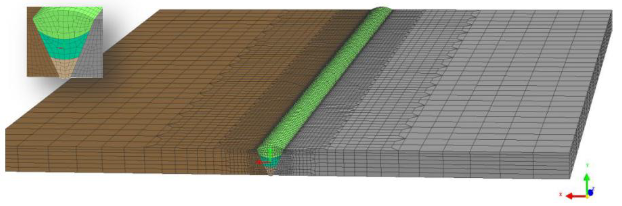
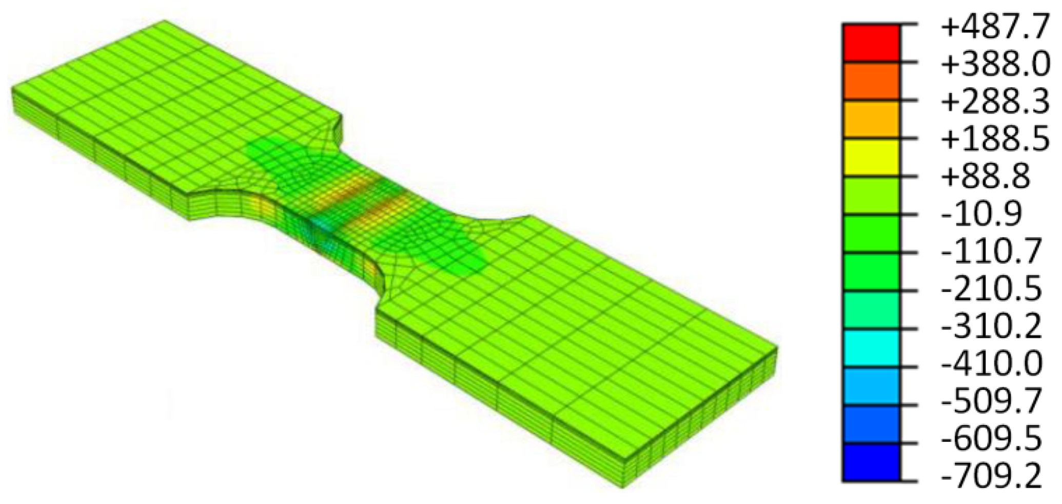
The numerical model, which is set-up for a structural weld simulation in case of the test series √area > 1000 µm, is presented in Figure 3. Thereby, the weld simulation is modeled in accordance to the real weld procedure including three single-sided weld passes; see left subfigure in Figure 3. Details to the applied material data, boundary conditions, as well as weld process parameters are provided in [30,47]. After structural weld simulation, the final specimen geometry is numerically cut-out of the weld array by eliminating the remaining elements in the model and the local residual stress state in the mid area of the sample, where the gas pores are located, is analyzed. Figure 4 demonstrates the residual stress condition in axial direction of the specimen, which shows values of around zero within the imperfected weld seam area. This comparably minor residual stress state can be explained by the single-sided three-pass weld procedure, which is significantly different to the double-sided two-pass welding in case of the test series √area < 1000 µm, leading to a local tempering of the central weld seam region due to the last weld pass at the top.
Within a prior study [49], a structural multi-pass weld simulation was performed, of which results also indicated that subsequent weld passes majorly affect the preceding ones leading to a relaxation of local residual stresses.
3.1.2. Fatigue Test Results
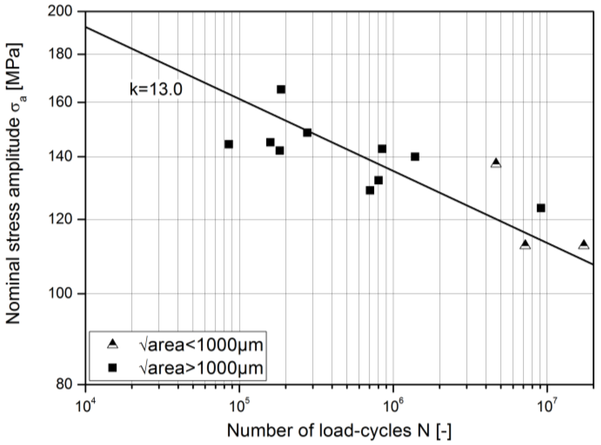
To evaluate the fatigue performance of the investigated weld samples, uniaxial fatigue tests at a frequency of 70 Hz and a load stress ratio of R = 0.1 utilizing a resonance test rig are performed. The abort criterion is burst fracture and the experimental fatigue test data is statistically evaluated utilizing the approach by ASTM E 739 [50]. Figure 5 depicts the nominal stress fatigue results and the statistically evaluated S/N-curve for a survival probability of PS = 50%. The slope in the finite life region is interpreted to k = 13.0 based on the method in [50], which is in sound accordance to the recommended value of k ~ 15.0 for mild steels in [51]. Subsequent to the cyclic testing, a detailed fracture surface analysis is conducted, of which results are provided in the next subsection. Based on these microscopic inspections, the fatigue test data points are separated in the two previously described test series, labeled as √area < 1000 µm and √area > 1000 µm, which act as comparison for the fatigue models later on. Further details regarding the fatigue tests are provided in [28] and [29,30], respectively. The statistical evaluation of the fatigue test data points reveals a scatter band in fatigue strength of a factor of 1.23 equaling the ratio of the nominal fatigue strength amplitude at PS = 10% to PS = 90%. As the position of the corresponding gas pores within the filler material varies, additionally the local residual stress value σres may not be totally equal in every case for both test series, which contributes to an increase of the scatter band considering all data points.
3.1.3. Fracture Surface Analysis
A detailed investigation of the fatigue fractured surfaces is performed utilizing light optical microscopy. Besides the evaluation of the crack initiation point as well as the area of fatigue crack propagation and burst fracture, special focus is laid on the characteristics of the gas pore imperfections within the weld metal to obtain geometric defect parameters such as size, shape, and location. Each detected pore is measured and the obtained data is used as basis for the application of the fatigue strength models. Subsequently, one example for each test series is illustrated to representatively show the difference in the fracture surfaces and gas pore dimensions between the two different sample types.
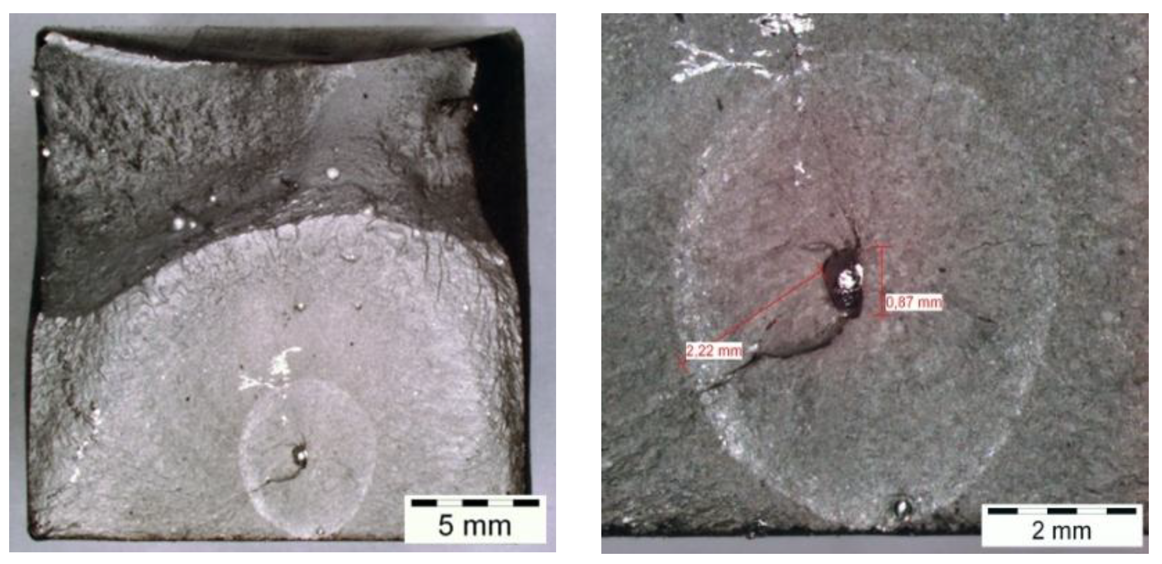
Figure 6 demonstrates a fracture surface of one characteristic sample from test series √area < 1000 µm. It is clearly observable that the fatigue crack originates at a gas pore in the middle-bottom section of the surface. A detailed analysis of this imperfection highlights that the maximum elongation of the pore measures about 0.87 mm and the √area-value of this roughly elliptical defect exhibits a value of 548 µm. Although other comparably smaller pores are monitored within the fractured surface, the fatigue crack initiates at this imperfection leading to a circular crack growth (bright area) up to burst fracture (dark area).
A summary of the measured pore sizes and positions for the test series √area < 1000 µm is provided in Table 4. Herein, the vertical distance to the top surface is given, which reveals that all gas pores are located within the interior region whereat the hardness measurements are performed. Additionally, all evaluated pores for both test series are roughly positioned at the axial midline of the sample without any deviation in horizontal direction towards the lateral edges. The calculated √area-values highlight that all imperfections are in the range of √area < 1000 µm with an average value of √area = 667 µm for all three gas pores.
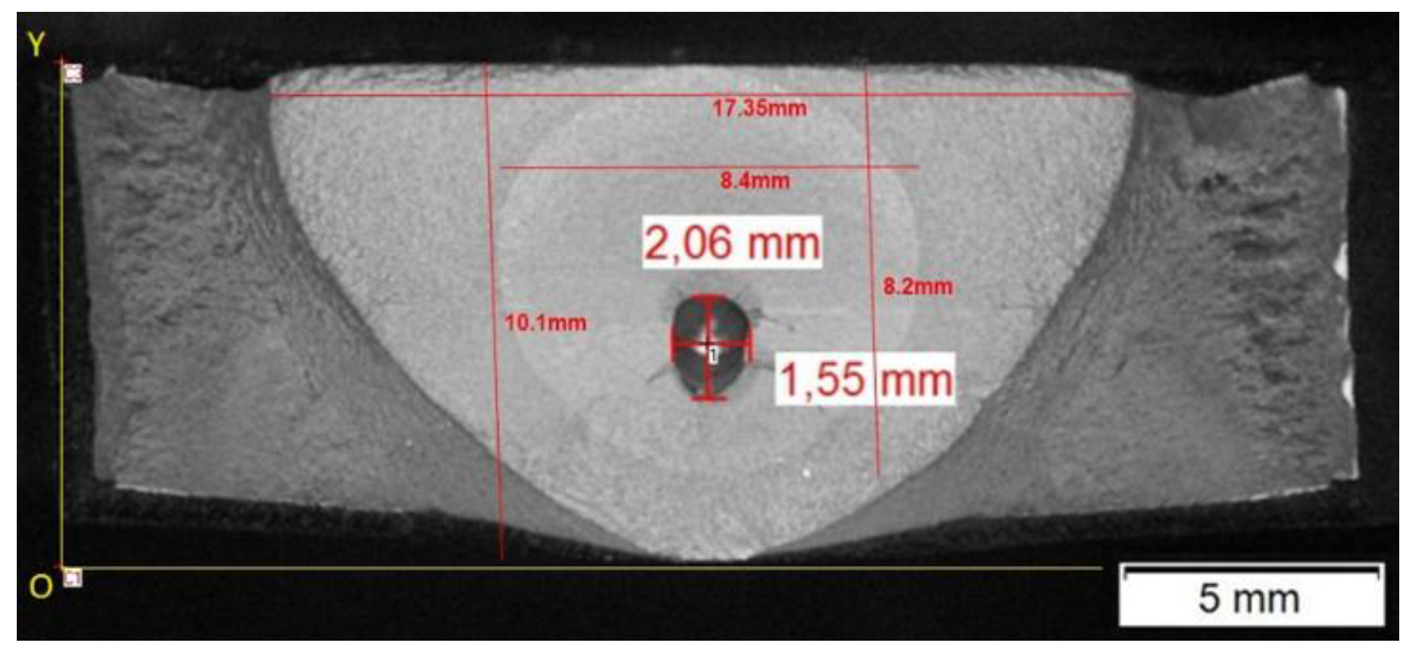
Similar findings are observed for one sample from test series √area > 1000 µm; see Figure 7. Compared to the imperfections of test series √area < 1000 µm, the gas pores are significantly larger in this case exhibiting a spherical or elliptical shape with a maximum elongation in the range of millimeters. The example in Figure 7 again demonstrates an approximately elliptical shape with dimensions of 2.06 mm and 1.55 mm for both main axes leading to a √area-value of about 3167 µm. Again, the fatigue crack originating at this defect maintains circular crack propagation (bright area) up to final burst fracture (dark areas) at both lateral sides of the fracture surface.
A summary of the measured pore sizes and positions for the test series √area > 1000 µm is provided in Table 5. The √area-values show that the gas pores are in the range of √area > 1000 µm with an average value of √area = 4462 µm for all ten gas pores.
In summary, the fatigue crack initiated at a gas pore for every cyclically tested weld sample, which highlights the importance to accurately assess the effect of such imperfections on the fatigue strength of welded joints. The gas pores are mainly located in the centre area of each specimen and no other surface-near defects are found as points of technical crack initiation. As the positions are not totally equal in each case, additionally the local residual state at the defects may exhibit a variation. As mentioned, this behavior affects the local fatigue-effective stress ratio Reff and may enhance the scatter band of the fatigue test data.
3.2. Fatigue Strength Assessment by Analytical Models
Within this section, the analytical fatigue models are applied. The approach utilized is that presented by Murakami [33] based on Equation (2) including the mean stress correction fmean by Equation (3), with the effective stress ratio Reff incorporating the local residual stress σres according to Equation (4). To estimate the alternating fatigue strength for a material without imperfections σf0, the introduced expression σf0 = 1.6 HV by [33,41] is applied. Based on this value and the fatigue model by Murakami, the critical defect size √area,c can be evaluated for each investigated test series below which no influence on the fatigue resistance by the gas pores is assumed.
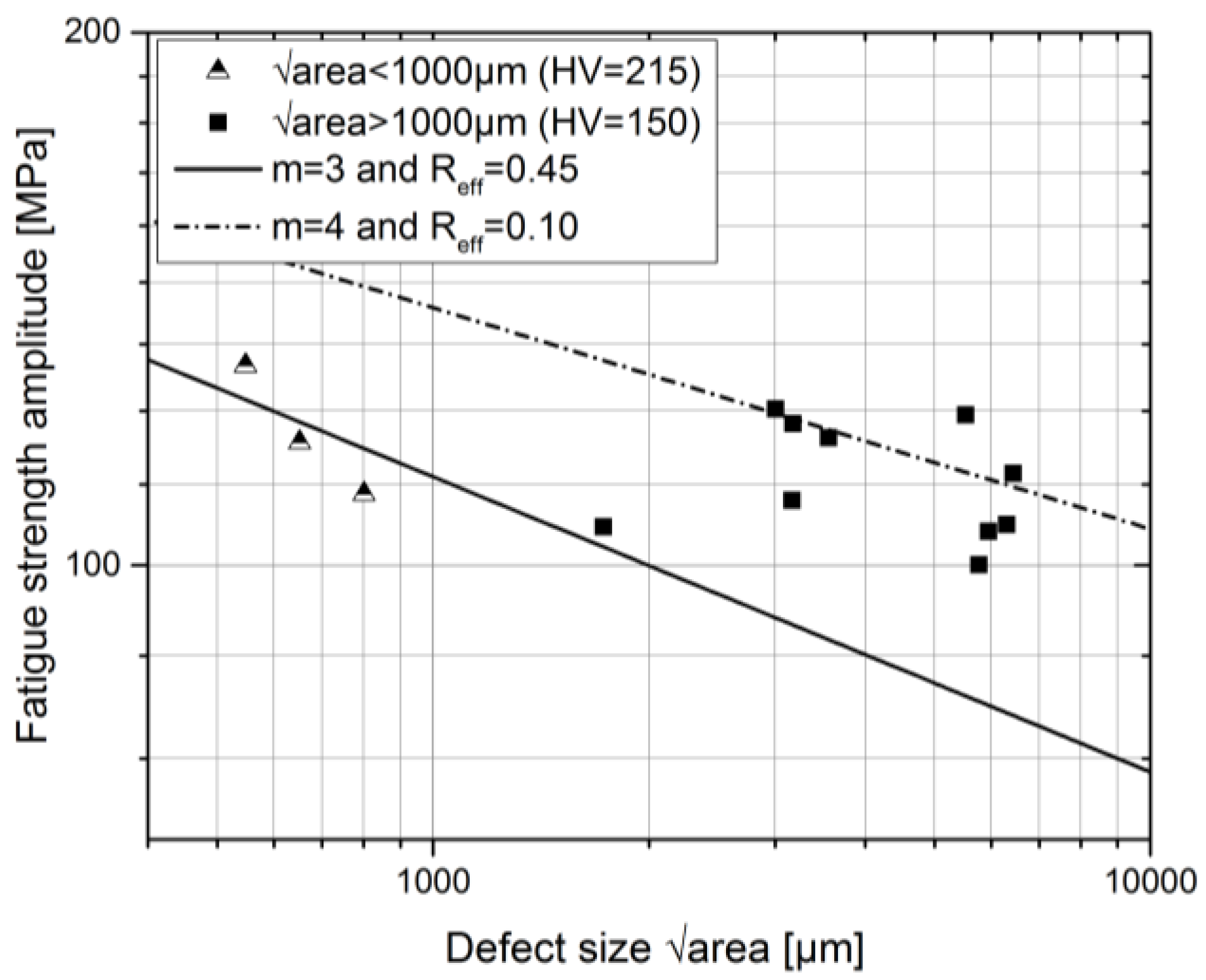
The results reveal that the critical defect sizes √area,c are significantly lower compared to the observed gas pores with √area,c-values of about 15 µm in case of the test series √area < 1000 µm and of about 100 µm for the test series √area > 1000 µm. Hence, the model by Murakami is well applicable to assess the fatigue strength of all detected gas pore sizes within this study. A comparison of the fatigue test data points to the estimated mean fatigue strength σf based on the fatigue model over √area is shown in Figure 8. Thereby, the fatigue strength amplitude is evaluated at a number of ten million load-cycles. As mentioned, a slope of 1/6 with m = 3 is applicable for defect sizes with √area < 1000 µm, which is shown to agree well with the fatigue tests data. As presented in [31], the slope may change depending on the gas pore size, considered either as a micro or macro defect. Hence, in the current investigation another slope value of m = 4 leading to a slope of 1/8 is applied, which seems to estimate the mean fatigue strength for defects with √area > 1000 µm more properly.
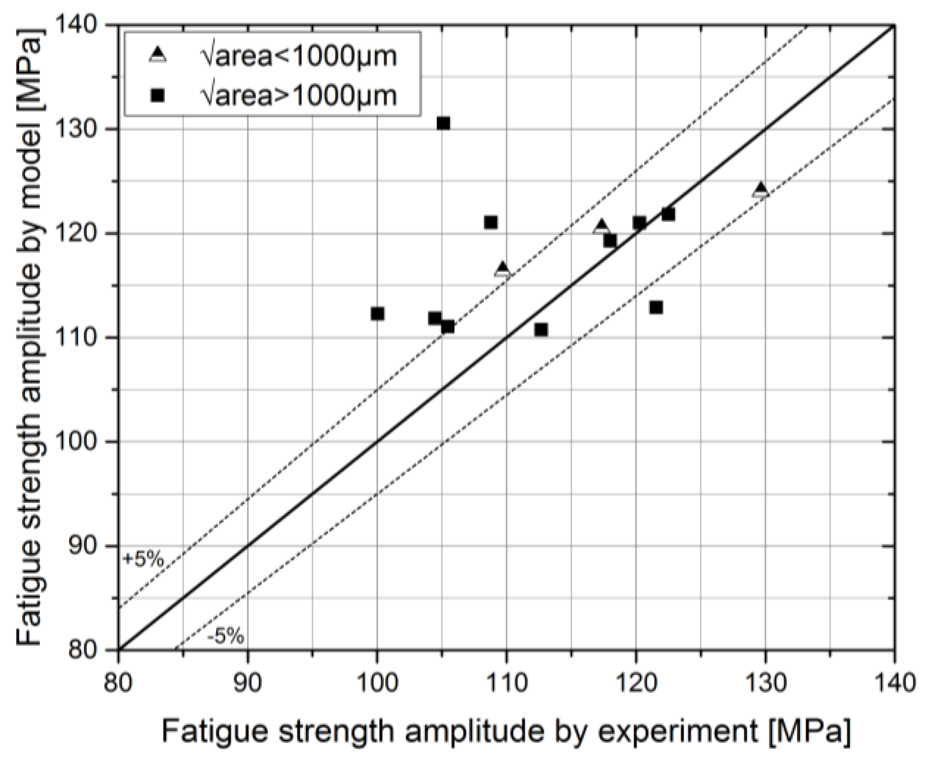
Figure 9 depicts the analytically evaluated fatigue strength amplitude by Murakami’s fatigue model compared to the experimental results utilizing the parameters m and Reff as presented in Figure 8. It is shown that this model properly estimates the fatigue resistance for the test series √area < 1000 µm with a mean deviation of only +1% compared to the experiments. In case of the larger defects with √area > 1000 µm, the estimated fatigue strength is again in sound accordance with the test results with a minor mean overestimation of +5% if a slope value of m = 4 is applied within the assessment. As aforementioned, scattering may arise by varying local residual stress states within the filler material depending on the pore location, which influences the fatigue-effective stress ratio. The presented pore size and location measurements reflect this assumption, which can be stated as the main reason for the scattering within this study. However, for statistical validation, further analysis should be performed in the future in order to incorporate the effect of the statistically distributed gas pore sizes and positions on the resulting fatigue strength.
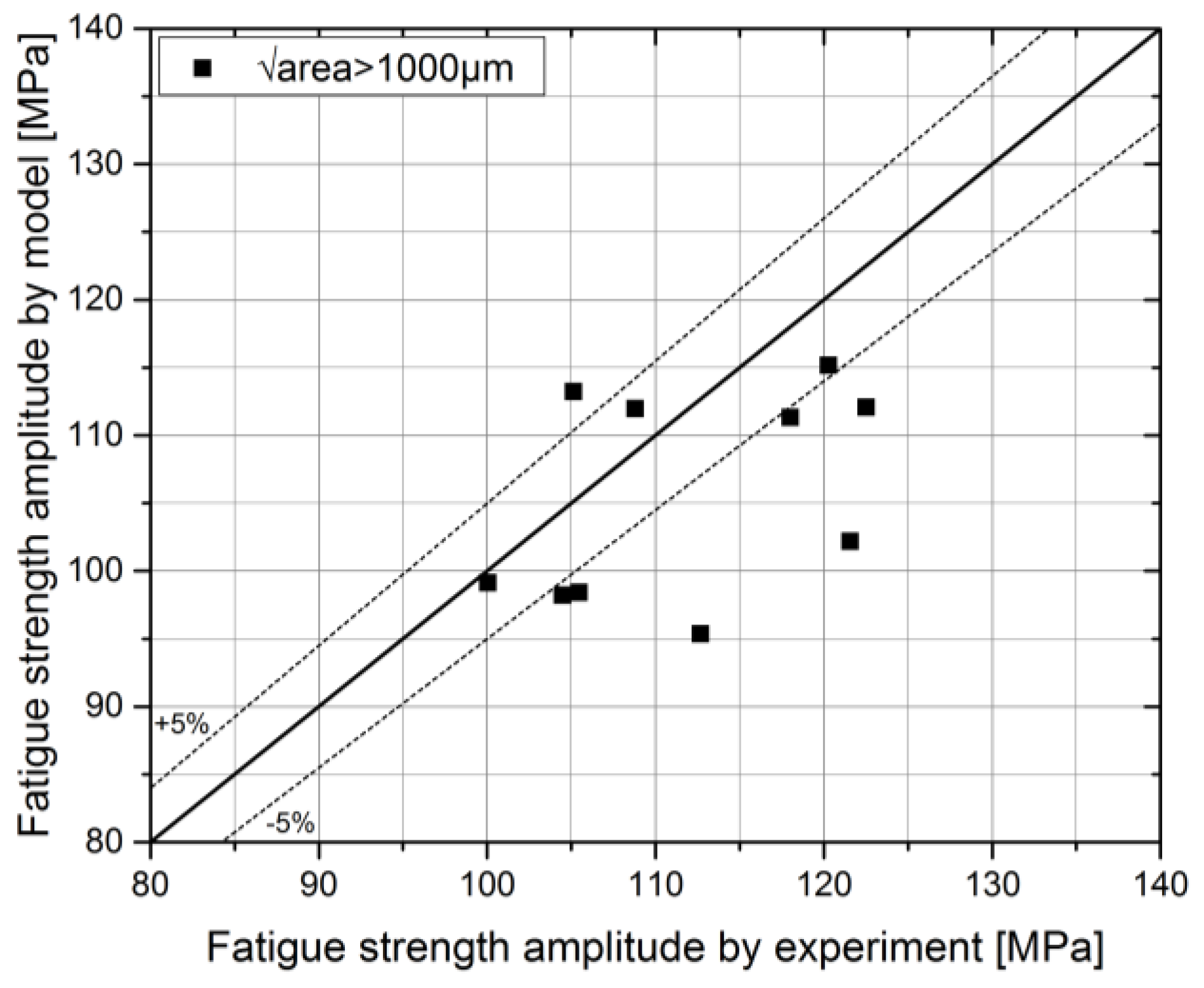
As the approach by De Kazinczy [39] is generally applicable for larger imperfections, this model, based on Equation (5), is only applied for the test series √area > 1000 µm considering Reff = 0.1; see Figure 10. Herein, a slightly more conservative assessment of the fatigue resistance is shown if utilizing this method, which leads to an average deviation of only −5% compared to the test results.
3.3. Fatigue Strength Assessment by Analytical/Numerical Approach
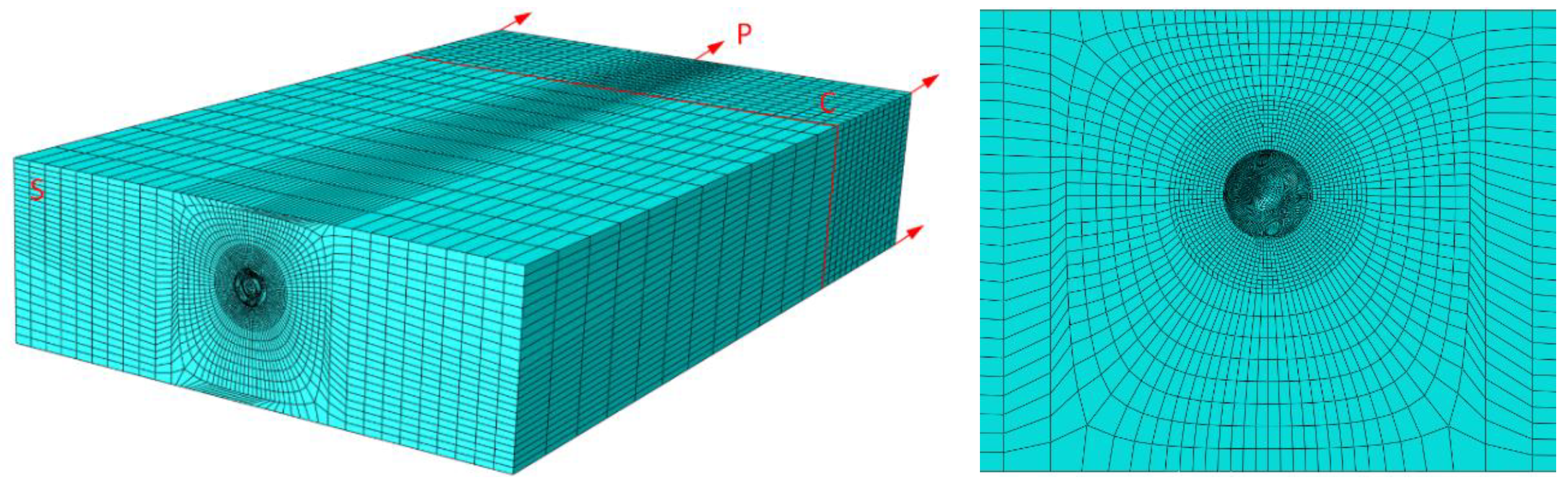
Within this section, the analytical fatigue strength model by Mitchell [43] based on Equation (6), featuring a numerical computation of the stress concentration factor Kt, is applied. Firstly, a half-symmetrical finite element model of a sample from test series √area > 1000 µm exhibiting a spherically shaped gas pore with a pore diameter of 1.95 mm in the middle of the cross section, is set-up; see Figure 11. The specimen is fixed at the clamping area C and the gas pore is modeled at the axial symmetry plane S in the front, which equals the boundary conditions for the samples at the fatigue tests. Linear-elastic material behavior with a Young’s modulus of 2.1 GPa and a Poisson’s ratio of ν = 0.3 for mild steel is used for the whole model. As no elastic-plastic analysis is required to evaluate Kt, a material mismatch within the welded zone is not considered. A structured, fine mesh, with an element size and type, according to a previous study [52], is utilized to accurately compute the local stress condition. A uniformly distributed tensile load of P = 1 MPa is applied at the rear surface to directly evaluate the stress concentration factor Kt by the numerical analysis.
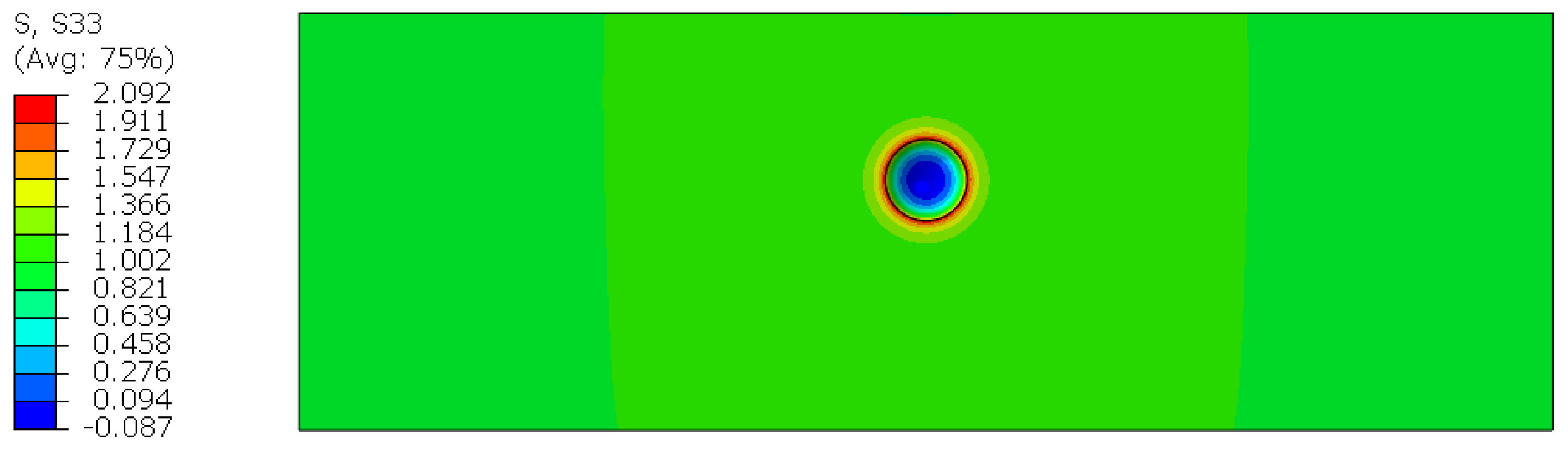
Figure 12 represents the stress value S33 in axial direction of the specimen as result of the numerical computation. It is shown that the stress concentration factor exhibits a value of Kt = 2.09, which is located around the edge of the spherical imperfection. The numerical result is in sound accordance to the analytical calculation based on Equation (7), which leads to a value of Kt = 2.05. Hence, the numerical model is well suitable to properly evaluate Kt for this comparably simple pore geometry, but it is also capable of computing stress concentrations for more complexly shaped imperfections.
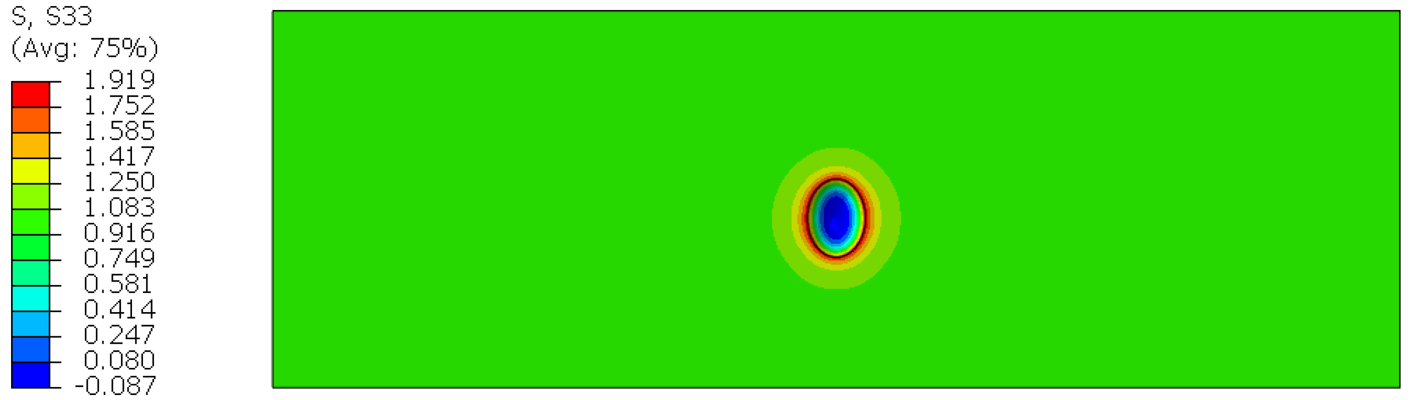
As example, the same numerical procedure is applied to an elliptically shaped gas pore of the test series √area > 1000 µm; see Figure 13. The size, shape, and location of the imperfection are taken from the fracture surface analysis presented in Figure 7. Again, the numerically computed stress S33 in axial direction shows a quite constant stress concentration around the edge of the gas pore with a value of Kt = 1.92. Applying the model by Mitchell based on Equation (6) and considering Reff = 0.1, the results reveal a sound match with a slightly conservative deviation of −5% compared to the tests.
4. Discussion
A comparison of the mean deviation by focusing on the incorporated analytical fatigue models with the experimental results is provided in Table 6. Herein, it is shown that the fatigue model by Murakami [33] is well applicable in case of imperfections exhibiting √area < 1000 µm with an average deviation of only +1%. In this case, the commonly applied slope value of m = 3 is utilized. To assess the fatigue strength of the gas pores with √area > 1000 µm, this value is modified to m = 4, which again demonstrates a sound conformity to the experiments with a mean overestimation of only +5%.
As the concept by De Kazinczy [39] based on Equation (5) is generally applicable for larger imperfections, it is only applied for the test series √area > 1000 µm. It assesses the fatigue strength with an average, slightly conservative, deviation of only −5% compared to the experiments. Overall, the analytical model by Murakami is well suitable to estimate the mean fatigue strength of both micro and macro pores, depending on the applied slope value within the assessment. The concept by De Kazinczy is also practicable to analytically evaluate the mean fatigue strength of comparably larger gas pores with √area > 1000 µm. In addition, it can be concluded that the applied mean stress correction according to Equation (3) is well eligible to consider both external mean stresses from the loading as well as the local residual stress state at the defect in terms of fatigue.
A detailed comparison of the fatigue assessment results for one comparably huge gas pore, taken from the fracture surface analysis of Figure 7, is presented in Table 7. In this specific case, Murakami’s √area approach maintains a non-conservative evaluation with an overestimation of +11% compared to the experiments utilizing a slope value of m = 4. The approach by De Kazinczy improves the assessment, but still leads to a slightly non-conservative fatigue strength estimation with a deviation of +3% to the experiments. Finally, the fatigue model by Mitchell [43] utilizing the numerically computed stress concentration factor Kt indicates a conservative assessment exhibiting only a minor deviation of −5% compared to the fatigue test results.
5. Conclusions
The results within this study show that gas pores significantly affect the fatigue strength of welded mild steel joints. Based on the conducted experiments and applied fatigue models, the following scientific as well as technological conclusions can be drawn:
- Internal imperfections, such as gas pores, significantly affect the fatigue strength of welded mild steel joints and should be considered within a fatigue assessment.
- The √area approach by Murakami [33] is well applicable to assess the mean strength of both micro and macroscopic gas pores depending on the applied slope value m. Within this study, it is presented that the recommended slope of 1/6 with m = 3 fits well to the defects with √area < 1000 µm, and m = 4 is well applicable for √area > 1000 µm.
- This work highlights that to properly assess the fatigue strength of welded mild steel joints containing internal imperfections, it is essential to incorporate fatigue-relevant local properties, such as the hardness and effective residual stress state.
Ongoing work focuses on the extension of these models towards fatigue assessment of high-strength steels considering various local defects, like undercuts [12] or porosity, as well as global imperfections, such as angular distortion or axial misalignment [53]. As only a limited number of welded specimens are investigated within this study, the investigation of the effect of statistically distributed gas pore sizes, shapes, and positions on the resulting fatigue strength is scheduled for prospective research.
Author Contributions
Martin Leitner performed the fatigue tests and accompanying analyses in case of the test series √area < 1000 µm, applied the presented fatigue strength models for all investigated data, evaluated and compared the results, and wrote the paper. Yukitaka Murakami contributed by scientific discussions of the findings and reviewing the article. Majid Farajian provided the fatigue test results and accompanying analyses data in case of the test series √area > 1000 µm, and assisted this research work. Heikki Remes and Michael Stoschka supported by reviewing the paper.
Acknowledgments
The financial support by the Austrian Federal Ministry for Digital and Economic Affairs and the National Foundation for Research, Technology and Development is gratefully acknowledged.
Conflicts of Interest
The authors declare no conflict of interest. The founding sponsors had no role in the design of the study; in the collection, analyses, or interpretation of data; in the writing of the manuscript; and in the decision to publish the results.
References
- Hou, C.-Y. Fatigue analysis of welded joints with the aid of real three-dimensional weld toe geometry. Int. J. Fatigue 2007, 29, 772–785. [Google Scholar] [CrossRef]
- Fricke, W. IIW guideline for the assessment of weld root fatigue. Weld. World 2013, 57, 753–791. [Google Scholar] [CrossRef]
- Sonsino, C.M. Effect of residual stresses on the fatigue behaviour of welded joints depending on loading conditions and weld geometry. Int. J. Fatigue 2009, 31, 88–101. [Google Scholar] [CrossRef]
- James, M.N.; Webster, P.J.; Hughes, D.J.; Chen, Z.; Ratel, N.; Ting, S.-P.; Bruni, G.; Steuwer, A. Correlating weld process conditions, residual strain and stress, microstructure and mechanical properties for high strength steel—The role of neutron diffraction strain scanning. Mater. Sci. Eng. A 2006, 427, 16–26. [Google Scholar] [CrossRef]
- James, M.N.; Ting, S.-P.; Bosi, M.; Lombard, H.; Hattingh, D.G. Residual strain and hardness as predictors of the fatigue ranking of steel welds. Int. J. Fatigue 2009, 31, 1366–1377. [Google Scholar] [CrossRef]
- Hobbacher, A. Recommendations for Fatigue Design of Welded Joints and Components; IIW Collection; Springer: Cham, Switzerland, 2016. [Google Scholar]
- Radaj, D.; Sonsino, C.M.; Fricke, W. Recent developments in local concepts of fatigue assessment of welded joints. Int. J. Fatigue 2009, 31, 2–11. [Google Scholar] [CrossRef]
- Stoschka, M.; Leitner, M.; Posch, G.; Eichlseder, W. Effect of high-strength filler metals on the fatigue behavior of butt joints. Weld. World 2013, 57, 85–96. [Google Scholar] [CrossRef]
- Stoschka, M.; Leitner, M.; Fössl, T.; Leitner, H.; Eichlseder, W. Application of fatigue approaches on fillet welds of high strength steel. Mater. Sci. Eng. Technol. 2010, 41, 961–971. [Google Scholar] [CrossRef]
- Barsoum, Z.; Jonsson, B. Influence of weld quality on the fatigue strength in seam welds. Eng. Fail. Anal. 2011, 18, 971–979. [Google Scholar] [CrossRef]
- Lillemäe, I.; Remes, H.; Liinalampi, S.; Itävuo, A. Influence of weld quality on the fatigue strength of thin normal and high strength steel butt joints. Weld. World 2016, 60, 731–740. [Google Scholar] [CrossRef]
- Ottersböck, M.; Leitner, M.; Stoschka, M.; Maurer, W. Effect of weld defects on the fatigue strength of ultra high-strength steels. Procedia Eng. 2016, 160, 214–222. [Google Scholar] [CrossRef]
- Kirkhope, K.J.; Bell, R.; Caron, L.; Basu, R.I.; Ma, K.-T. Weld detail fatigue life improvement techniques. Part 1: Review. Mar. Struct. 1999, 12, 447–474. [Google Scholar] [CrossRef]
- Leitner, M.; Stoschka, M.; Eichlseder, W. Fatigue enhancement of thin-walled, high-strength steel joints by high-frequency mechanical impact treatment. Weld. World 2014, 58, 29–39. [Google Scholar] [CrossRef]
- Leitner, M.; Stoschka, M.; Schanner, R.; Eichlseder, W. Influence of High Frequency Peening on Fatigue of High-Strength Steels. FME Trans. 2012, 40, 99–104. [Google Scholar]
- Leitner, M.; Barsoum, Z.; Schäfers, F. Crack propagation analysis and rehabilitation by HFMI of pre-fatigued welded structures. Weld. World 2016, 60, 581–592. [Google Scholar] [CrossRef]
- Leitner, M.; Mössler, W.; Putz, A.; Stoschka, M. Effect of post-weld heat treatment on the fatigue strength of HFMI-treated mild steel joints. Weld. World 2015, 59, 861–873. [Google Scholar] [CrossRef]
- Jonsson, B.; Samuelsson, J.; Marquis, G.B. Development of Weld Quality Criteria Based on Fatigue Performance. Weld. World 2011, 55, 79–88. [Google Scholar] [CrossRef]
- Jonsson, B.; Dobmann, G.; Hobbacher, A.; Kassner, M.; Marquis, G.B. IIW Guidelines on Weld Quality in Relationship to Fatigue Strength; IIW Collection; Springer: Cham, Switzerland, 2016. [Google Scholar]
- Zhu, M.-L.; Xuan, F.-Z.; Du, Y.-N.; Tu, S.-T. Very high cycle fatigue behavior of a low strength welded joint at moderate temperature. Int. J. Fatigue 2012, 40, 74–83. [Google Scholar] [CrossRef]
- Yeom, H.; Choi, B.; Seol, T.; Lee, M.; Jeon, Y. Very High Cycle Fatigue of Butt-Welded High-Strength Steel Plate. Metals 2017, 7, 103. [Google Scholar] [CrossRef]
- Chan, K.S. Roles of microstructure in fatigue crack initiation. Int. J. Fatigue 2010, 32, 1428–1447. [Google Scholar] [CrossRef]
- Sangid, M.D. The physics of fatigue crack initiation. Int. J. Fatigue 2013, 57, 58–72. [Google Scholar] [CrossRef]
- Bayraktar, E.; Garcias, I.M.; Bathias, C. Failure mechanisms of automotive metallic alloys in very high cycle fatigue range. Int. J. Fatigue 2006, 28, 1590–1602. [Google Scholar] [CrossRef]
- Shen, F.; Zhao, B.; Li, L.; Chua, C.K.; Zhou, K. Fatigue damage evolution and lifetime prediction of welded joints with the consideration of residual stresses and porosity. Int. J. Fatigue 2017, 103, 272–279. [Google Scholar] [CrossRef]
- Gou, G.; Zhang, M.; Chen, H.; Chen, J.; Li, P.; Yang, Y.P. Effect of humidity on porosity, microstructure, and fatigue strength of A7N01S-T5 aluminum alloy welded joints in high-speed trains. Mater. Des. 2015, 85, 309–317. [Google Scholar] [CrossRef]
- Tsay, L.W.; Shan, Y.-P.; Chao, Y.-H.; Shu, W.Y. The influence of porosity on the fatigue crack growth behavior of Ti–6Al–4V laser welds. J. Mater. Sci. 2006, 41, 7498–7505. [Google Scholar] [CrossRef]
- Leitner, M.; Murakami, Y.; Remes, H.; Stoschka, M. Damage Tolerant Fatigue Design of Seam Imperfections in Mild Steel Butt Joints by Analytical and Numerical Approaches; International Institute of Welding (IIW): Yutz, France, XIII-WG4-158-17; 2017. [Google Scholar]
- Javaheri, E.; Hemmesi, K.; Tempel, P.; Farajian, M. Fatigue Assessment of the Welded Joints Containing Process Relevant Imperfections; International Institute of Welding (IIW): Yutz, France, XIII-2477-13; 2013. [Google Scholar]
- Farajian, M.; Fenzl, R.; Beckmann, C.; Tempel, P.; Kranz, B.; Wagner, S.; Siegele, D. Quantifizierung des Einflusses der Nahtqualität auf die Ermüdungsfestigkeit von Schweißverbindungen; Report number IGF-17.559B/DVS-Nr. 09.055; Fraunhofer-Institut für Werkstoffmechanik IWM: Halle, Germany, 2016. (In German) [Google Scholar]
- McEvily, A.J.; Endo, M.; Murakami, Y. On the √area relationship and the short crack fatigue threshold. Fatigue Fract. Eng. Struct. 2003, 26, 269–278. [Google Scholar] [CrossRef]
- Murakami, Y.; Kodama, S.; Konuma, S. Quantitative Evaluation of Effects of Nonmetallic Inclusions on Fatigue Strength of High Strength Steel. Trans. Jpn. Soc. Mech. Eng. Eng. A 1988, 54, 688–696. [Google Scholar] [CrossRef]
- Murakami, Y. Metal Fatigue: Effects of Small Defects and Non-Metallic Inclusions; Elsevier: New York, NY, USA, 2002. [Google Scholar]
- Baumgartner, J.; Bruder, T. Influence of weld geometry and residual stresses on the fatigue strength of longitudinal stiffeners. Weld. World 2013, 57, 841–855. [Google Scholar] [CrossRef]
- Kihl, D.P.; Sarkani, S. Mean stress effects in fatigue of welded steel joints. Prob. Eng. Mech. 1999, 14, 97–104. [Google Scholar] [CrossRef]
- Leitner, M. Influence of effective stress ratio on the fatigue strength of welded and HFMI-treated high-strength steel joints. Int. J. Fatigue 2017, 102, 158–170. [Google Scholar] [CrossRef]
- Beretta, S.; Blarasin, A.; Endo, M.; Giunti, T.; Murakami, Y. Defect tolerant design of automotive components. Int. J. Fatigue 1997, 19, 319–333. [Google Scholar] [CrossRef]
- Costa, N.; Machado, N.; Silva, F.S. A new method for prediction of nodular cast iron fatigue limit. Int. J. Fatigue 2010, 32, 988–995. [Google Scholar] [CrossRef]
- De Kazinczy, F. Effect of small defects on the fatigue properties of medium strength cast steel. J. Iron Steel Inst. 1970, 851–855. [Google Scholar]
- Radaj, D. Geometriekorrektur zur Spannungsintensität an elliptischen Rissen. Schw. Schneid. 1977, 29, 398–402. (In German) [Google Scholar]
- Casagrande, A.; Cammarota, G.P.; Micele, L. Relationship between fatigue limit and Vickers hardness in steels. Mater. Sci. Eng. A 2011, 528, 3468–3473. [Google Scholar] [CrossRef]
- Pavlina, E.J.; van Tyne, C.J. Correlation of Yield Strength and Tensile Strength with Hardness for Steels. J. Mater. Eng. Perform. 2008, 17, 888–893. [Google Scholar] [CrossRef]
- Mitchell, M.R. Review of the Mechanical Properties of Cast Steels with Emphasis on Fatigue Behavior and the Influence of Microdiscontinuities. J. Eng. Mater. Technol. 1977, 329–343. [Google Scholar] [CrossRef]
- Davis, T.; Healy, D.; Bubeck, A.; Walker, R. Stress concentrations around voids in three dimensions: The roots of failure. J. Struct. Geol. 2017, 102, 193–207. [Google Scholar] [CrossRef]
- Ostsemin, A.A.; Utkin, P.B. Stress-Concentration Coefficients of Internal Welding Defects. Rus. Eng. Res. 2008, 28, 1165–1168. [Google Scholar] [CrossRef]
- Rossini, N.S.; Dassisti, M.; Benyounis, K.Y.; Olabi, A.G. Methods of measuring residual stresses in components. Mater. Des. 2012, 35, 572–588. [Google Scholar] [CrossRef] [Green Version]
- Leitner, M.; Simunek, D.; Shah, F.S.; Stoschka, M. Numerical fatigue assessment of welded and HFMI-treated joints by notch stress/strain and fracture mechanical approaches. Adv. Eng. Softw. 2016, accepted-in press. [Google Scholar] [CrossRef]
- Alipooramirabad, H.; Paradowska, A.; Ghomashchi, R.; Kotousova, A.; Reid, M. Quantification of residual stresses in multi-pass welds using neutron diffraction. J. Mater. Process. Technol. 2015, 226, 40–49. [Google Scholar] [CrossRef]
- Ottersböck, M.; Stoschka, M.; Thaler, M. Study of kinematic strain hardening law in transient welding simulation. In Mathematical Modelling of Weld Phenomena; Montanuniversität Leoben: Leoben, Austria, 2014; Volume 10, pp. 255–266. [Google Scholar]
- ASTM International. Standard practice for statistical analysis of linear or linearized stress-life (S-N) and strain-life (e-N) fatigue data; ASTM E739-91(1998); ASTM International: West Conshohocken, PA, USA, 1998. [Google Scholar]
- McKelvey, S.A.; Lee, Y.-L.; Barkey, M.E. Stress-Based Uniaxial Fatigue Analysis Using Methods Described in FKM-Guideline. J. Fail. Anal. Prev. 2012, 12, 445–484. [Google Scholar] [CrossRef]
- Leitner, M.; Pauer, P.; Kainzinger, P.; Eichlseder, W. Numerical effects on notch fatigue strength assessment of non-welded and welded components. Comp. Struct. 2017, 191, 51–61. [Google Scholar] [CrossRef]
- Ottersböck, M.; Leitner, M.; Stoschka, M.; Maurer, W. Analysis of fatigue notch effect due to axial misalignment for ultra high-strength steel butt joints; International Institute of Welding (IIW): Yutz, France, XIII-2690-17; 2017. [Google Scholar]
Figure 1.
Representation of weld array and specimen geometry for test series √area < 1000 µm [28].
Figure 1.
Representation of weld array and specimen geometry for test series √area < 1000 µm [28].

Figure 2.
Hardness measurement paths from center of weld seam and results for √area < 1000 µm.

Figure 3.
Numerical model for structural weld simulation in case of test series √area > 1000 µm [30].
Figure 3.
Numerical model for structural weld simulation in case of test series √area > 1000 µm [30].

Figure 4.
Resulting residual stress state in axial direction of the specimen geometry (in MPa) [30].
Figure 4.
Resulting residual stress state in axial direction of the specimen geometry (in MPa) [30].

Figure 5.
Fatigue test results and statistically evaluated S/N-curve for PS = 50%.

Figure 6.
Example of fracture surface for test series √area < 1000 µm [28].
Figure 6.
Example of fracture surface for test series √area < 1000 µm [28].

Figure 7.
Example of fracture surface for test series √area > 1000 µm [30].
Figure 7.
Example of fracture surface for test series √area > 1000 µm [30].

Figure 8.
Fatigue strength amplitude based on model by Murakami [33] compared to test data.
Figure 8.
Fatigue strength amplitude based on model by Murakami [33] compared to test data.

Figure 9.
Comparison of fatigue strength amplitude by experiments to model by Murakami [33].
Figure 9.
Comparison of fatigue strength amplitude by experiments to model by Murakami [33].

Figure 10.
Comparison of fatigue strength amplitude by experiments to model by De Kazinczy [39].
Figure 10.
Comparison of fatigue strength amplitude by experiments to model by De Kazinczy [39].

Figure 11.
Model of specimen from test series √area > 1000 µm including a spherical gas pore.

Figure 12.
Numerically computed axial stress S33 for spherical gas pore.

Figure 13.
Numerically computed axial stress S33 for ellipsoidal gas pore of Figure 7.
Figure 13.
Numerically computed axial stress S33 for ellipsoidal gas pore of Figure 7.


Table 1.
Overview of investigated test series.
| Denotation | Weld type | Weld-Passes | Area (w by t) | Reference |
|---|---|---|---|---|
| √area < 1000 µm | Butt joint | Two, double-sided | 20 by 16 mm | [28] |
| √area > 1000 µm | Butt joint | Three, single-sided | 30 by 10 mm | [29] |
Table 2.
Chemical composition of mild steel S355 in weight %.
| Material | C | Mn | Si | P | S | Cr | Ni | Fe | Reference |
|---|---|---|---|---|---|---|---|---|---|
| S355NL | 0.09 | 1.29 | 0.02 | 0.010 | 0.013 | 0.039 | 0.036 | balance | [30] |
Table 3.
Mean hardness and residual stress condition of investigated weld samples.
| Denotation | Hardness Value (HV5) | Axial Residual Stress (MPa) |
|---|---|---|
| √area < 1000 µm | 215 | approximately 335 |
| √area > 1000 µm | 150 | around zero |
Table 4.
Measured pore sizes and positions for test series √area < 1000 µm.
| Length of Gas Pore (mm) | Width of Gas Pore (mm) | Calculated √area (µm) | Vertical Distance from Top Surface (mm) |
|---|---|---|---|
| 0.87 | 0.44 | 548 | 3.5 |
| 0.76 | 0.71 | 651 | 5.1 |
| 1.08 | 0.76 | 801 | 4.2 |
Table 5.
Measured pore sizes and positions for test series √area > 1000 µm.
| Length of Gas Pore (mm) | Width of Gas Pore (mm) | Calculated √area (µm) | Vertical Distance from Top Surface (mm) |
|---|---|---|---|
| 2.06 | 1.55 | 3167 | 5.4 |
| 1.95 | 1.95 | 1728 | 3.9 |
| 2.05 | 1.40 | 3003 | 7.3 |
| 3.14 | 3.10 | 5530 | 6.3 |
| 2.12 | 1.90 | 3557 | 6.8 |
| 4.20 | 3.14 | 6437 | 6.3 |
| 3.58 | 2.96 | 5770 | 3.8 |
| 3.72 | 3.03 | 5951 | 4.0 |
| 1.79 | 1.79 | 3173 | 5.9 |
| 3.69 | 3.43 | 6306 | 5.8 |
Table 6.
Mean deviation of analytical fatigue models compared to experiments.
| Denotation | Murakami [33] | De Kazinczy [39] |
|---|---|---|
| √area < 1000 µm | +1% | - |
| √area > 1000 µm | +5% | −5% |
Table 7.
Deviation of fatigue models compared to experimental result for pore of Figure 7.
© 2018 by the authors. Licensee MDPI, Basel, Switzerland. This article is an open access article distributed under the terms and conditions of the Creative Commons Attribution (CC BY) license (http://creativecommons.org/licenses/by/4.0/).
Share and Cite
MDPI and ACS Style
Leitner, M.; Murakami, Y.; Farajian, M.; Remes, H.; Stoschka, M. Fatigue Strength Assessment of Welded Mild Steel Joints Containing Bulk Imperfections. Metals 2018, 8, 306. https://doi.org/10.3390/met8050306
AMA Style
Leitner M, Murakami Y, Farajian M, Remes H, Stoschka M. Fatigue Strength Assessment of Welded Mild Steel Joints Containing Bulk Imperfections. Metals. 2018; 8(5):306. https://doi.org/10.3390/met8050306
Chicago/Turabian StyleLeitner, Martin, Yukitaka Murakami, Majid Farajian, Heikki Remes, and Michael Stoschka. 2018. "Fatigue Strength Assessment of Welded Mild Steel Joints Containing Bulk Imperfections" Metals 8, no. 5: 306. https://doi.org/10.3390/met8050306
Note that from the first issue of 2016, this journal uses article numbers instead of page numbers. See further details here.