Acoustic Emission Signatures of Fatigue Damage in Idealized Bevel Gear Spline for Localized Sensing

1
Civil and Materials Engineering, University of Illinois at Chicago, Chicago, IL 60607, USA
2
Naval Air Systems Command (NAVAIR), Patuxent River, MD 20670, USA
*
Author to whom correspondence should be addressed.
Metals 2017, 7(7), 242; https://doi.org/10.3390/met7070242
Submission received: 30 May 2017
/
Revised: 26 June 2017
/
Accepted: 26 June 2017
/
Published: 30 June 2017
(This article belongs to the Special Issue Advanced Non-Destructive Testing in Steels)
Abstract
:In many rotating machinery applications, such as helicopters, the splines of an externally-splined steel shaft that emerges from the gearbox engage with the reverse geometry of an internally splined driven shaft for the delivery of power. The splined section of the shaft is a critical and non-redundant element which is prone to cracking due to complex loading conditions. Thus, early detection of flaws is required to prevent catastrophic failures. The acoustic emission (AE) method is a direct way of detecting such active flaws, but its application to detect flaws in a splined shaft in a gearbox is difficult due to the interference of background noise and uncertainty about the effects of the wave propagation path on the received AE signature. Here, to model how AE may detect fault propagation in a hollow cylindrical splined shaft, the splined section is essentially unrolled into a metal plate of the same thickness as the cylinder wall. Spline ridges are cut into this plate, a through-notch is cut perpendicular to the spline to model fatigue crack initiation, and tensile cyclic loading is applied parallel to the spline to propagate the crack. In this paper, the new piezoelectric sensor array is introduced with the purpose of placing them within the gearbox to minimize the wave propagation path. The fatigue crack growth of a notched and flattened gearbox spline component is monitored using a new piezoelectric sensor array and conventional sensors in a laboratory environment with the purpose of developing source models and testing the new sensor performance. The AE data is continuously collected together with strain gauges strategically positioned on the structure. A significant amount of continuous emission due to the plastic deformation accompanied with the crack growth is observed. The frequency spectra of continuous emissions and burst emissions are compared to understand the differences of plastic deformation and sudden crack jump. The correlation of the cumulative AE events at the notch tip and the strain data is used to predict crack growth. The performance of the new sensor array is compared with the conventional AE sensors in terms of signal to noise ratio and the ability to detect fatigue cracking.
1. Introduction
The function of the gearbox in a helicopter transmission system is to keep the engine torque stable at optimum levels and transmit the power. As the spline section of the gearbox is subjected to externally-cyclic loading (e.g., torque, tensile and bend), it is susceptible to develop fatigue cracks and spalling [1,2,3]. Being a non-redundant component, it is important to monitor the structural state of the spline section using real-time and non-intrusive nondestructive evaluation (NDE) methods. There are several NDE methods implemented to monitor gearbox components, including vibration, acoustic emission, and debris monitoring. For instance, Hussain and Gabbar [4] developed a real-time coded genetic algorithm to detect gear faults, and optimized the process of vibration response feature extraction by band-pass and wavelet filters. Lin et al. [5] studied the signature of spectrograms of vibration signals caused by the crack evolution in gear in terms of B-spline wavelet method. Liu et al. [6] diagnosed the faults in the gearbox according to the vibration signal by means of an empirical mode decomposition and Hilbert spectrum. Bonnardot et al. [7] tracked the rotation behavior of a gearbox based on resampling the acceleration signals. Leturiondo et al. [8] evaluated the condition of the gearbox based on the physics-based model. In their model, not only the dynamics of the rolling element bearings have been considered, but also the influence of the electrical process is included. The change in the gear-mesh stiffness obtained from the vibration signals is typically correlated with the presence of cracking [9,10,11]. Though the vibration method is a well-established method for monitoring rotating machinery, the sensitivity is insufficient for detecting the initiation of a fatigue crack. Additionally, the operational conditions (e.g., background noises and rotational speed) may influence the baseline vibration properties [12]. Acoustic emission (AE) is a passive NDE method for detecting the active flaws in the gearbox components. The AE method is based on detecting elastic waves released by sudden localized failures (e.g., crack growth, corrosion) and applied in damage detection in various metallic components. Typically, the AE sensors are mounted on the structural surface, which requires elastic waves propagating through several structural layers before reaching the sensor from the crack location in complex structures [13]. While the AE characteristics of the prescribed minor and major defects on the tooth are identified by several researchers [14,15], the applicability of their test results in a realistic condition is questionable as the AE waveform depends on the source function, the structural geometry, and the sensors used. It is important to place AE sensors in proximity to the source in order to reduce the influence of the structural geometry on AE waveforms [16]. The AE and vibration methods have been combined in the literature in order to increase the damage detection ability (e.g., [17,18,19,20,21,22]). Although there are many laboratory-scale studies aiming to the spline section of gearbox, the application of the method in a realistic field test is challenged by the complexity of AE signal, and the influence of background noise on the dataset. However, the representative AE features obtained in a properly designed laboratory scale experiment can help us to understand the characteristics of AE signal generated by the fatigue testing for localized sensing [23,24]. The majority of the studies studied simple plate geometry [25]; however, the complexity in structural geometry would affect the AE signature.
The major goals of this study are (1) to identify the AE signatures due to fatigue crack growth released in the complex geometry of a spline section; and (2) to test a new piezoelectric sensor array with the ability to place the sensor array inside the gearbox to reduce the wave propagation path. To achieve the research goals, the geometrical details of spline section are built in a flattened geometry. The sample is loaded under constant cycle fatigue until the crack length reaches about 7 mm. The AE signatures related to two major source mechanisms as plastic deformation and sudden crack jump are identified. The performance of the piezoelectric sensor array is evaluated in terms of detecting the crack growth in comparison with conventional AE sensors.
The outline of this paper is as follows: A brief introduction to the AE method relevant to this study is presented in Section 2. The details of fatigue testing and AE setting are described in Section 3. The numerical model to predict the crack growth behavior is described in Section 4. Section 5 includes the experimental results, and the conclusions of this study are presented in Section 6.
2. Acoustic Emission Method
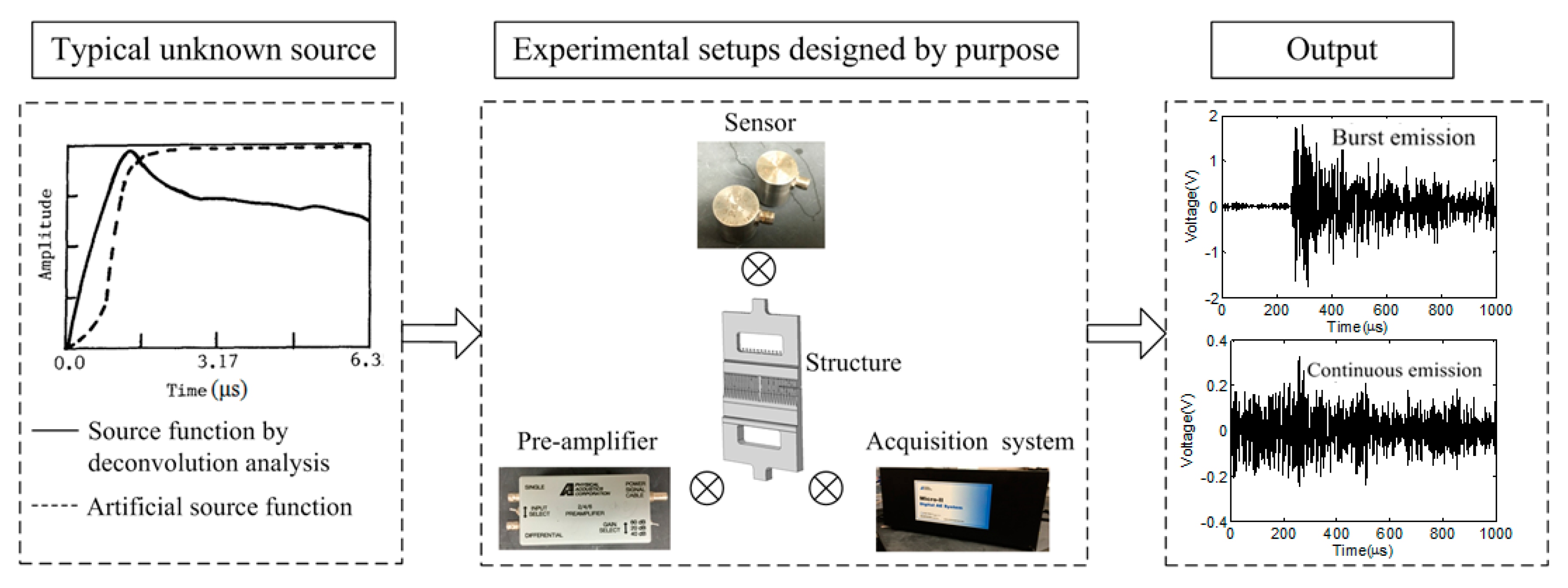
Acoustic emission (AE) is the phenomenon of radiation of transient elastic waves in a material when the sudden redistribution of the stress occurs in the material [26]. As the AE sensors (typically piezoelectric types) are triggered by the transient elastic waves released from sudden localized failure, the method is called a ‘passive’ NDE method. Figure 1 illustrates the measurement chain of an AE signal. In essence, the quantitative AE method requires understanding and modeling all components in Figure 1. The AE signal is the convolution of AE source mechanism, medium transfer function, and sensor transfer function. The data acquisition system should also be considered if it applies analog/digital filters or gain.
The AE source mechanism is controlled by materials (e.g., metals, composites), loading types (e.g., monotonic or fatigue), loading rates (e.g., fast or slow), and the previous load history of the material. Currently, a number of studies have attempted to identify the source mechanisms for different materials and loading conditions. Theoretical studies are inspired by the application of seismology. The body force equivalents representing dislocations were derived theoretically [27], and the crack kinetics and kinematics were studied by means of the moment tensor analysis [28,29,30]. However, the derived source is the representative acoustic emission; the difference between AE waves due to generalized theory and those of cracking has not been clearly realized. The source mechanism is significantly influenced by the material composition [31,32,33,34,35,36]. For instance, sources associated with composites are matrix cracking, fiber-matrix debonding, fiber pull-out, fiber bridging, inter-ply failure, delamination, and fiber breakage. For brittle materials, such as concrete or rock, microcrack and macrocrack initiation and growth are two major AE sources. For metallic materials, the source mechanisms are usually related to the microstructural changes such as movement of dislocation, slip, twinning, fracture, and debonding of precipitates, in addition to macrostuctural changes, such as crack jump.
The common sources that generate AE signals in the spline section of gearbox include plastic deformation, microfracture, wear, bubbles, friction, and impact [37]. Different source mechanisms release different energy levels, which affect their detectability by the AE method. If the signal level is below electronic or background noise level, the AE method cannot detect the flaw. Poddar and Giurgiutiu [38] applied the numerical method to understand the detectable length of fatigue cracking by means of AE. Therefore, it is important to identify detectable source mechanisms and adapt them in a realistic test environment. In this study, the structural material is made of steel, and the target source mechanisms are plastic deformation and sudden crack jump.
Once the AE signals are detected, there are different signal processing techniques to extract features describing source mechanisms [20,39,40,41]. For instance, Siracusano et al. [42] conducted the Hilbert-Huang transform on the AE signals to evaluate the damage evolution in the cementitious material, and the method has been applied successfully in plain and reinforced concrete, and the AE behavior of nucleation of micro-cracks and the formation of macro-cracks are identified. Hamzah et al. [43] found the correlation between the lubricating condition of the gearbox and RMS (root mean square) level. While the relationships between damage states of the gearbox and AE features have been established by several researchers [44,45,46,47], the results are based on laboratory-scale experiments with artificially introduced damage. Additionally, almost all of the AE features are related to the burst types of signals (as shown in Figure 1), and the continuous signals are typically considered as noise sources in detecting fatigue crack growth.
3. Overview of the Idealized Gearbox Sample
The spline section of the helicopter gearbox has complex geometry with variable cross-sections, as shown in Figure 2a. The structural complexity affects the wave field and propagation when the crack occurs at a spline tooth. Therefore, it is important to test a similar geometry under fatigue loading for understanding the characteristics of AE signals due to fatigue cracking. However, it is difficult to apply fatigue loading on a cylinder-shaped spline in the laboratory environment. In this study, the cylindrical geometry is flattened while the cross-sectional details and splines are preserved (see in Figure 2b). The idealization makes it possible to conduct a fatigue test and initiate and grow the fatigue crack. The cross-sectional profile of the idealized gearbox sample is shown in Figure 2c. The window section is specifically designed to place the new piezoelectric sensor array, which would have a direct path between the crack and sensing element, similar to its planned installment inside the gearbox. The idealized specimen is manufactured using a structural steel plate. A notch with a length of 7.6 cm was formed at the spline section in order to grow the crack within the capacity of the loading machine. The AE signal is influenced by the crack growth direction relative to the sensor position. The laboratory condition that crack growth is perpendicular to the piezoelectric sensor array simulates the actual field condition.
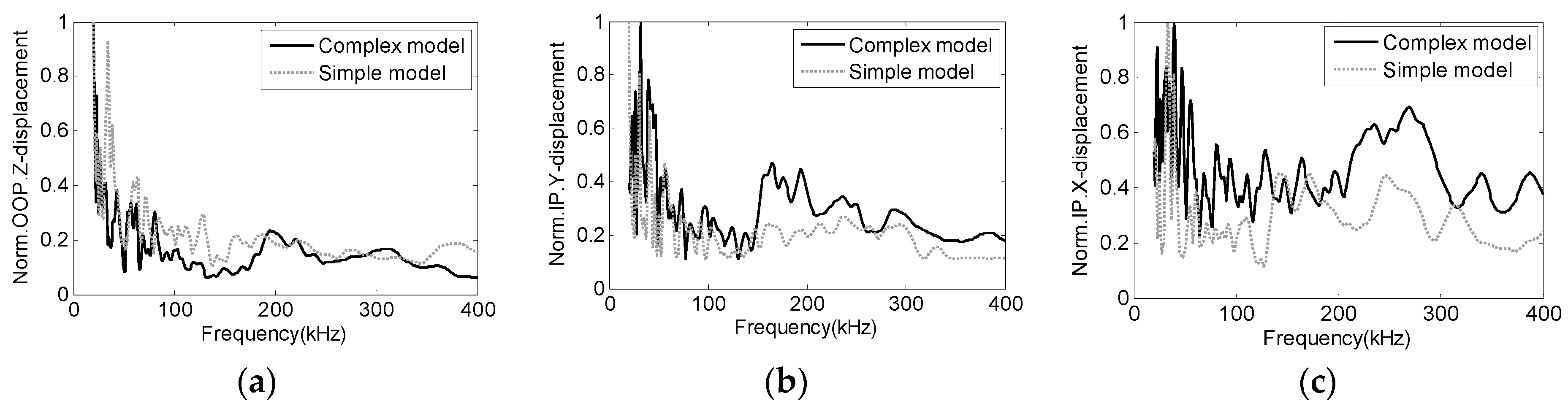
In order to show the influence of geometric details (e.g., cross-section and spline), two finite elements models using COMSOL Multiphysics software (Version 4.2a, COMSOL Inc., Stockholm, Sweden) are built, and the frequency analysis is conducted to illustrate the influence of geometric details on the elastic wave propagation. A tetrahedral mesh is implemented with the minimum mesh size of 0.25 mm to order to achieve 1 MHz resolution. The numerical model is simulated in the frequency domain by applying harmonic perturbation at the location of the notch. The natural boundary condition is defined. The material properties of steel are defined as the Young’s modulus (200 GPa), density (7850 kg/m3), and Poisson’s ratio (0.33). One model preserves all the spline details in a typical helicopter gearbox, and the other model has a uniform surface without spline components, as shown in Figure 3. The constant amplitude dipole force is introduced as an artificial AE source, and a sweep of the frequency range from 20 kHz to 400 kHz, with a frequency step of 1 kHz, is applied to find the structural response in the frequency domain. The comparison of the displacement responses at the selected point (position of the AE sensor highlighted as the wideband (WD) sensor on the figure) is shown in Figure 4. The geometric details cause the different characteristics of the AE signal, especially in the high-frequency range (150 kHz to 300 kHz). The difference is more apparent for in-plane responses (x and y directions) because the dipole force is applied on the surface, which coincides with the in-plane direction. The numerical results indicate that the test structure should preserve as many geometrical details as possible to obtain acoustic signatures representing a given damage mode and structural component.
4. Experimental Design
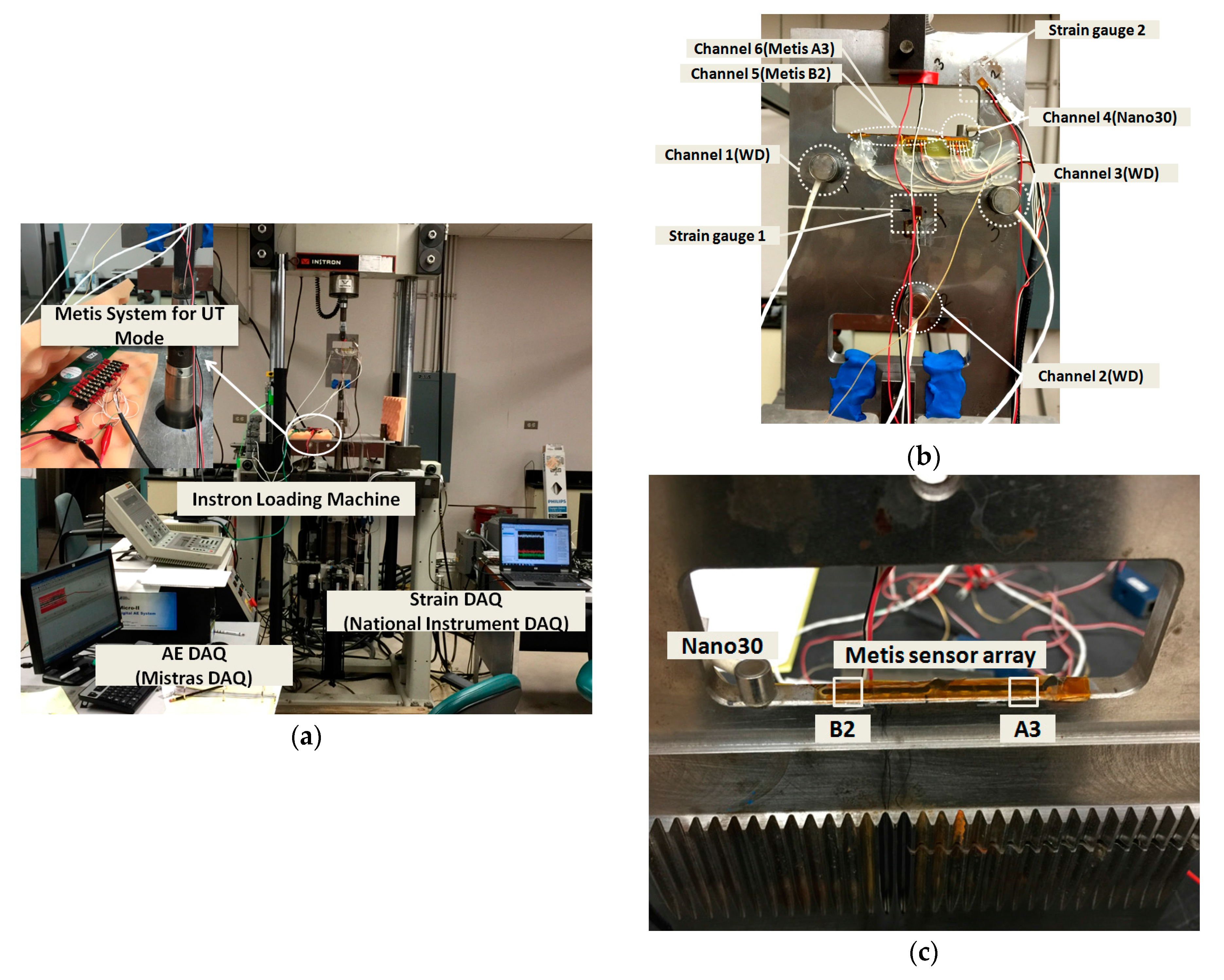
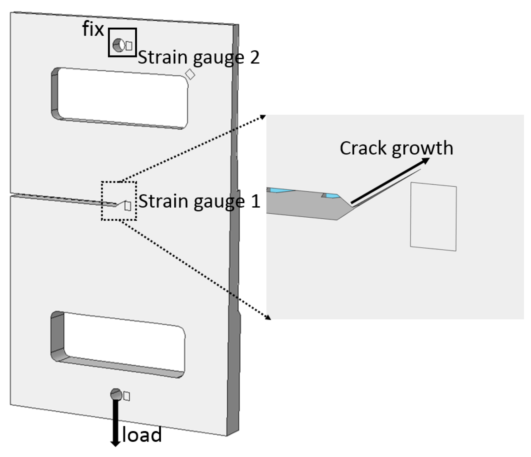
The experimental setup includes three monitoring technologies: AE, strain, and ultrasonics. The AE data is recorded using six piezoelectric sensors: three WD sensors (wideband sensor manufactured by Mistras Group Inc., Princeton Junction, NJ, USA) placed in a triangulation form for source localization; one Nano 30 sensor (nano-30 FP 97 sensor manufactured by Mistras Group Inc., Princeton Junction, NJ, USA) placed in the windowed section, and two piezoelectric wafer sensors as part of a new sensor array (manufactured by Metis Design Inc., Boston, MA, USA) named as B2 and A3 sensors. WD sensors were also utilized at the field testing conducted at the NAVAIR facility where the sensors were attached to the gearbox housing [48]. A Nano 30 sensor has a frequency response of 100–400 kHz, and the required contact size in order to fit into the windowed section. Piezoelectric wafer sensors have been well established in the literature [49]. The sensors have disk-like geometry with the dimensions of 3 mm diameter and 0.5 mm thickness, a flat frequency response up to MHz frequencies, and operate in d31 mode. All of the sensors are bonded using super glue and connected to 40 dB gain pre-amplifiers. The sensor couplant condition is preserved until the completion of the experiments. The AE data is collected using PCI-8 data acquisition board manufactured by Mistras Group Inc. The major data acquisition variables are the digital filter, as 20–400 kHz, hit definition time, as 800 μs, hit lockout time, as 1200 μs, and 50–70 dB threshold level depending on the hit rate (discussed in detail below). AE waveforms are recorded with a 3 MHz sampling rate with a duration of 1 ms. Two strain gauges manufactured by Micro Measurements are positioned on the notch tip and the corner of the windowed section (see Figure 5b). The strain data is collected using a National Instruments data acquisition system and the LabView program. The strain calibration is conducted at the beginning of each test. In addition to AE and strain sensors, a new piezoelectric sensor array designed by Metis Design Inc. is placed on the windowed section, as shown in Figure 5c, for ultrasonic and AE modes. The array has two actuators and six receivers in order to map the damage state of spline section using guided wave ultrasonics. Receivers are used as AE sensors during fatigue testing, and UT data is collected when the specimen is under no load. In this paper, only the results of AE and strain data are presented.
The experimental setup is shown in Figure 5a. The fatigue test was performed using an Instron loading machine. The fatigue load setting was a 4 Hz frequency with max/min load ratio of 0.1 and a maximum load of 12 kN. One specimen was tested until the crack length reached 7 mm at 590,211 cycles. The experiments were conducted about four to five hours of each day (total of eight days and 43 h).
The flattened bevel sample is modeled using Franc3D software (Version 7.0.8, Fracture Analysis Consultants Inc., New York, NY, USA) to identify the crack growth characteristics. The Franc3D model of the sample is shown in Figure 6a including all of the details, the prescribed notch, and its mesh are shown in Figure 6b. Figure 6b shows the image of the predicted crack growth direction, which agrees well with the experimental result. The stress intensity factors due to 1000 lb (4.5 kN) loading along different crack surfaces are shown in Figure 6c–e. Based on the fracture model and observation in the test, the predicted crack growth rate for 12 kN loading is 12.7 × 10⁻⁶ mm/cycle. The crack length after about 550,000 cycles is calculated as 7 mm. The direction of crack growth and the crack growth rate obtained through Franc3D shows good agreement with experimental observation as discussed in Section 5.
5. Results
The AE data are analyzed using 2D localization, individual waveforms, and time/frequency domain features. The characteristics of AE signals are evaluated in order to determine the precursor of crack growth. The strain history is combined with the AE data in order to validate the initiation time of the crack growth. The performance of new piezoelectric sensors is evaluated by comparing with the waveforms of a Nano 30 sensor. The major questions sought in the experimental results are:
- What are the typical AE waveforms representing fatigue crack growth developed in the complex geometry of the spline section?
- What are the precursor AE signatures indicating the initiation of fatigue crack?
- Is the sensitivity of miniaturized wafer type piezoelectric sensor sufficient to operate as an AE sensor?
5.1. AE Waveforms Representing Fatigue Crack
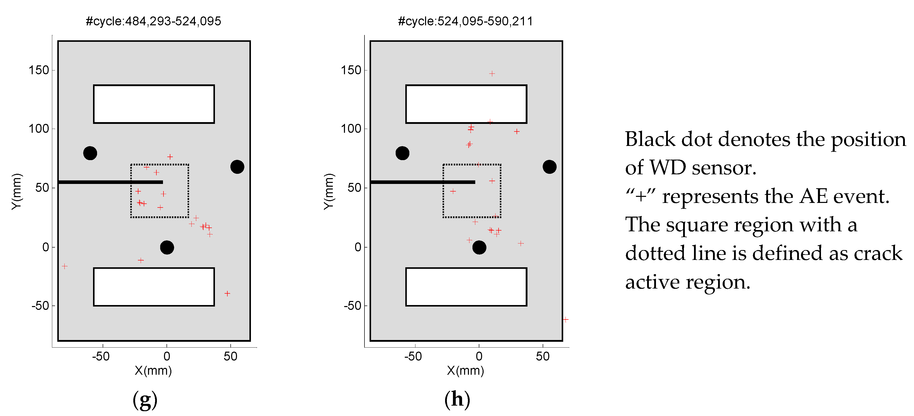
As the AE sensors are highly sensitive to secondary emissions, such as friction, it is important to reliably identify the AE waveforms representing the fatigue crack growth by source localization and the comparison of the AE data with other monitoring data. As 2D source localization requires minimum three sensors in order to locate the source, an AE event (defined as AE signals resulted in a meaningful location by the localization algorithm) is more reliably linked with source mechanisms than individual AE hits (defined as any AE signal above the threshold level). In this study, three WD sensors are placed in a triangular form to localize the AE source as shown in Figure 7. The inputs to the source localization algorithm are wave velocity, sensor positions, and arrival time differences. The prescribed wave speed is determined as 3000 m/s based on the pencil lead break (PLB) simulations. The cluster analysis is performed within 25 mm × 25 mm window in the vicinity of the notch tip, and the AE events occurred in this region are considered as the AE related to the fatigue crack growth. The selection of a fixed wave velocity, fixed threshold to determine the arrival time, and a fixed cluster window limits the target AE events as dominated by surface waves within the energy release similar to PLB. If AE signal is strong such that the first threshold crossing is a longitudinal wave, the located event will be outside the cluster window, which is then considered only in total AE events. The size of cluster is selected to allow ±12.5 mm error in source localization, which corresponds to approximately one wavelength. Figure 7 shows the AE events detected within the different ranges of the fatigue cycles. At the beginning of the fatigue test, almost every event occurred in the top pin area, and those events were identified as the frictions of near pin location. After the pin was replaced, no event was detected. With the increase of the fatigue cycles, the AE event accumulation was observed near the cluster window.
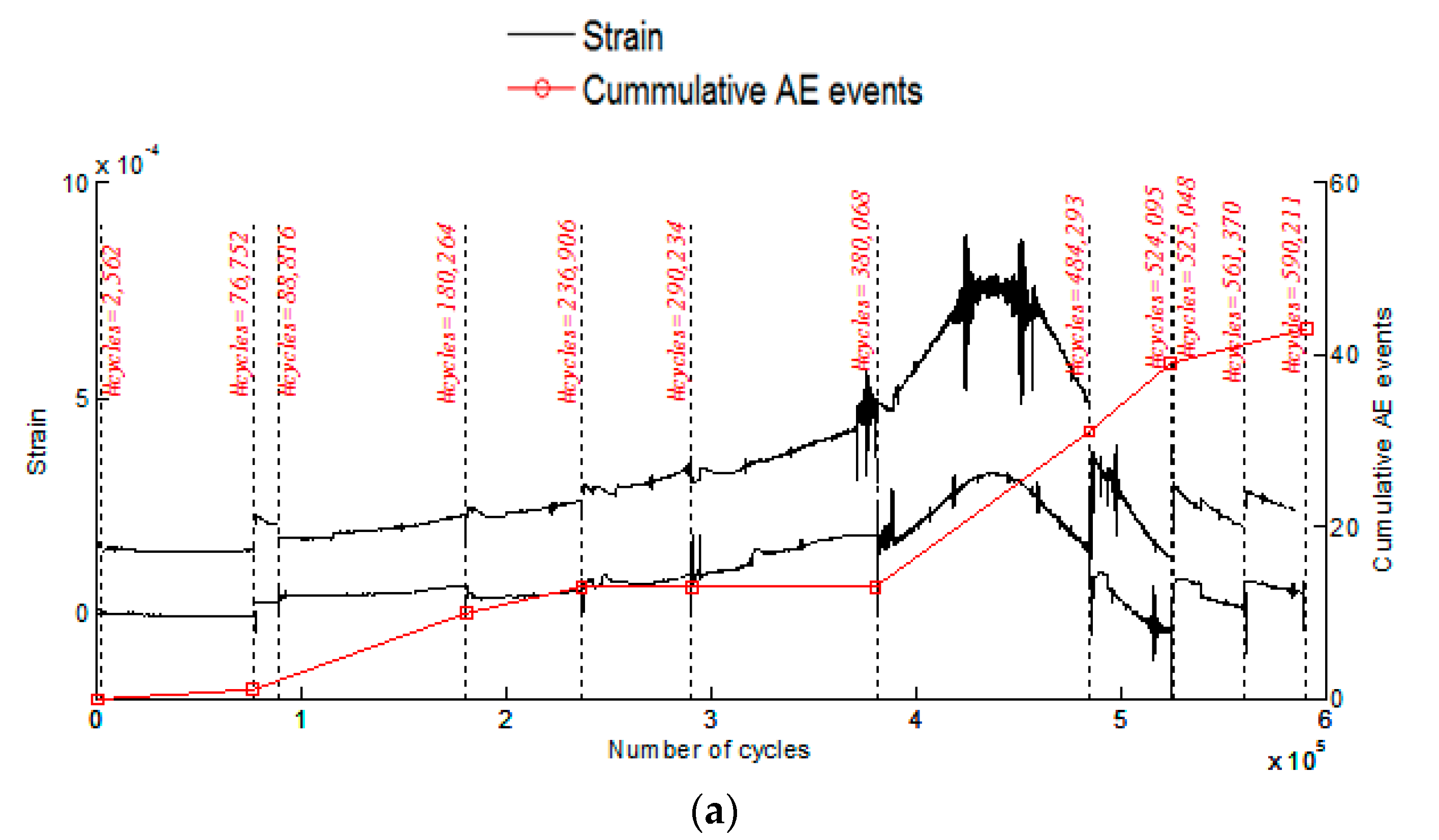
It is also important to verify that the accumulations of AE events at the notch tip are related to fatigue crack growth using the strain history. Figure 8 shows the minimum and maximum envelops of strain levels throughout the fatigue testing for strain gauge 1 located near the crack tip and strain gauge 2 located near the window edge (labeled in Figure 5). The amplitude of strain gauge 1 increases abruptly at the end of 380,068 fatigue cycles, while strain gauge 2 has stable response throughout the testing. The peak value of strain gauge 1 occurs between the fatigue cycles of 380,068–484,293. The sudden increase of the strain level near the notch tip is considered as a result of plastic strain accumulation before the crack jump. Once the crack tip passes the strain gauge location, the surface that strain gauge is attached to is exposed to the compression zone, as observed in the strain envelope.
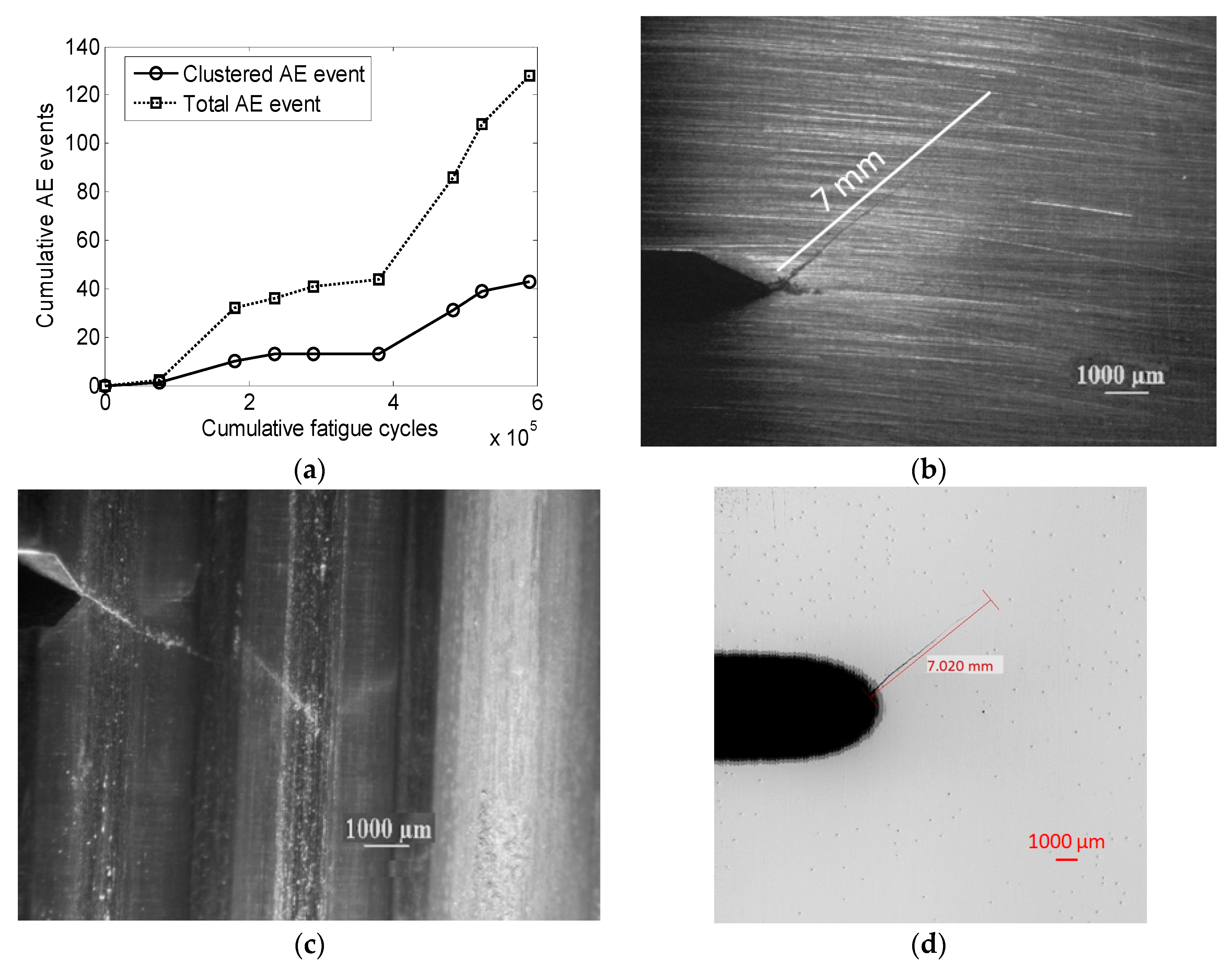
Figure 9a shows the total AE events and the AE events within the cluster window shown in Figure 7 versus the cumulative fatigue cycles. The total AE events throughout test are 128 (43 in the cluster window). There is a significant increase in the cumulative AE events after about 380,068 cycles, which coincides with the increase of strain near the crack tip as shown in Figure 8. The major crack growth behavior is observed between 380,068–590,211 cycles. A microscopic image of crack growth observed after 590,211 cycles are shown in Figure 9b,c. The crack direction agrees with the numerical result as discussed in Section 4. In order to get the more accurate crack length, we used the Sonoscan Gen 6 C-SAM acoustic microscope to scan the sample. The sensor with 100 MHz is used, and the resolution can be up to 60 μm. The region of crack is shown in Figure 9d, and the length of the crack is 7.020 mm.
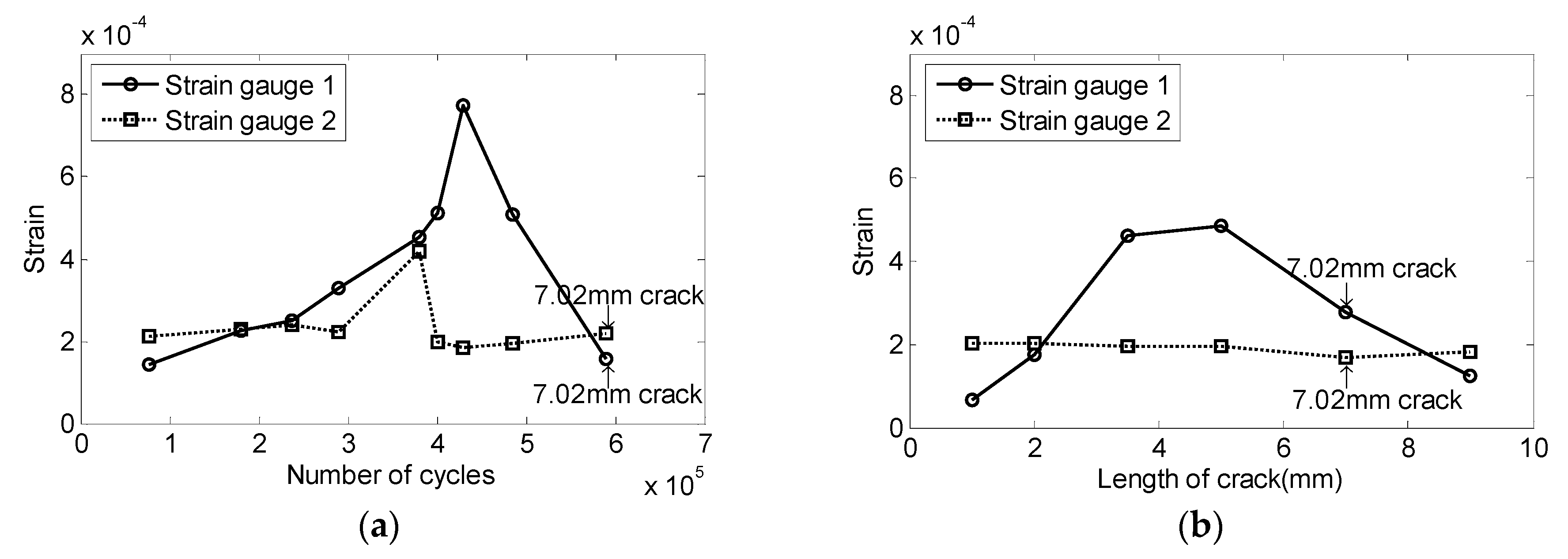
The crack length data is only recorded at the end of the experiments. In order to find the crack growth behavior, a numerical model is built to find the strain values at the locations of strain gauges when the crack length increases. The steel sample with different crack lengths of 1 mm, 2 mm, 5 mm, and 7.02 mm is modeled, as shown in Figure 10, and loaded with the maximum load applied experimentally. The numerical and experimental strain values are compared in Figure 11. Although the numerical strain of strain gauge 1 is smaller than that the experimental results, the results of strain gauge 2 shows good agreement. The details of crack model would influence the absolute strain distribution near the crack tip. The numerical results indicate that the strain of strain gauge 1 drops once the crack length exceeds the position of strain gauge 1, which agrees well with the experimental results.
Once the AE accumulation near the notch tip is verified as representing the crack growth, an AE event located near the notch tip and occurred near 400,000 cycles is selected for further analysis. Figure 12 shows the time domain histories and their frequency spectra of three WD sensors detected by the same event. While three sensors have similar transfer functions, their waveforms show differences. The amplitude of sensor 2 is higher, and the response of sensor 3 shows higher dispersive behavior. While the material is isotropic, sensor-source direction influences the waveforms detected by the AE sensors. While the time domain signals are not similar, the frequency domain responses show similar broadband behavior. The frequency centroids of sensor 1 to sensor 3 are 224.5 kHz, 264.6 kHz, and 245.1 kHz, respectively. On the other hand, peak frequencies also depend on the sensor-source direction. For instance, the peak frequencies of sensor 1 to sensor 3 are 105.8 kHz, 258.2 kHz, and 144.7 kHz, respectively. Similar behavior is observed for the other events detected in the cluster window.
5.2. Precursor AE Signature
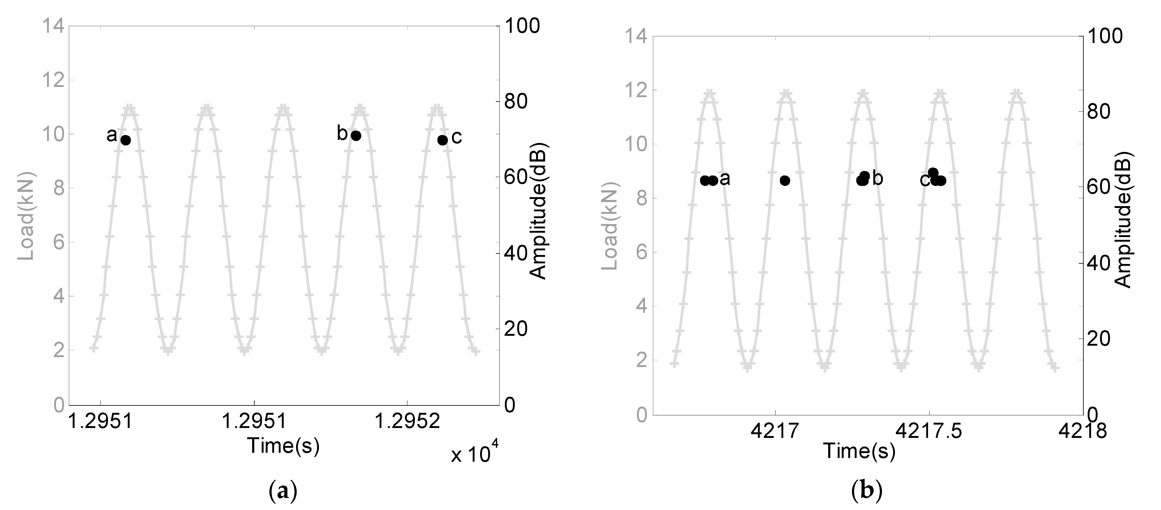
The fatigue test was continued for about five to six hours of testing each day. A pattern of increasing continuous emission was observed after about 237,000 cycles. It is considered that the increase of continuous emission from the notch tip is a precursor indication of sudden crack growth jumps. Figure 13 shows five fatigue cycles of different test days and the amplitudes of AE hits recorded at the selected fatigue cycles. Three continuous emissions that occurred near the peak load are selected from each dataset, and labeled on the figure. The majority of the AE hits near the peak load are detected by sensor 3, which is located across from the notch tip.
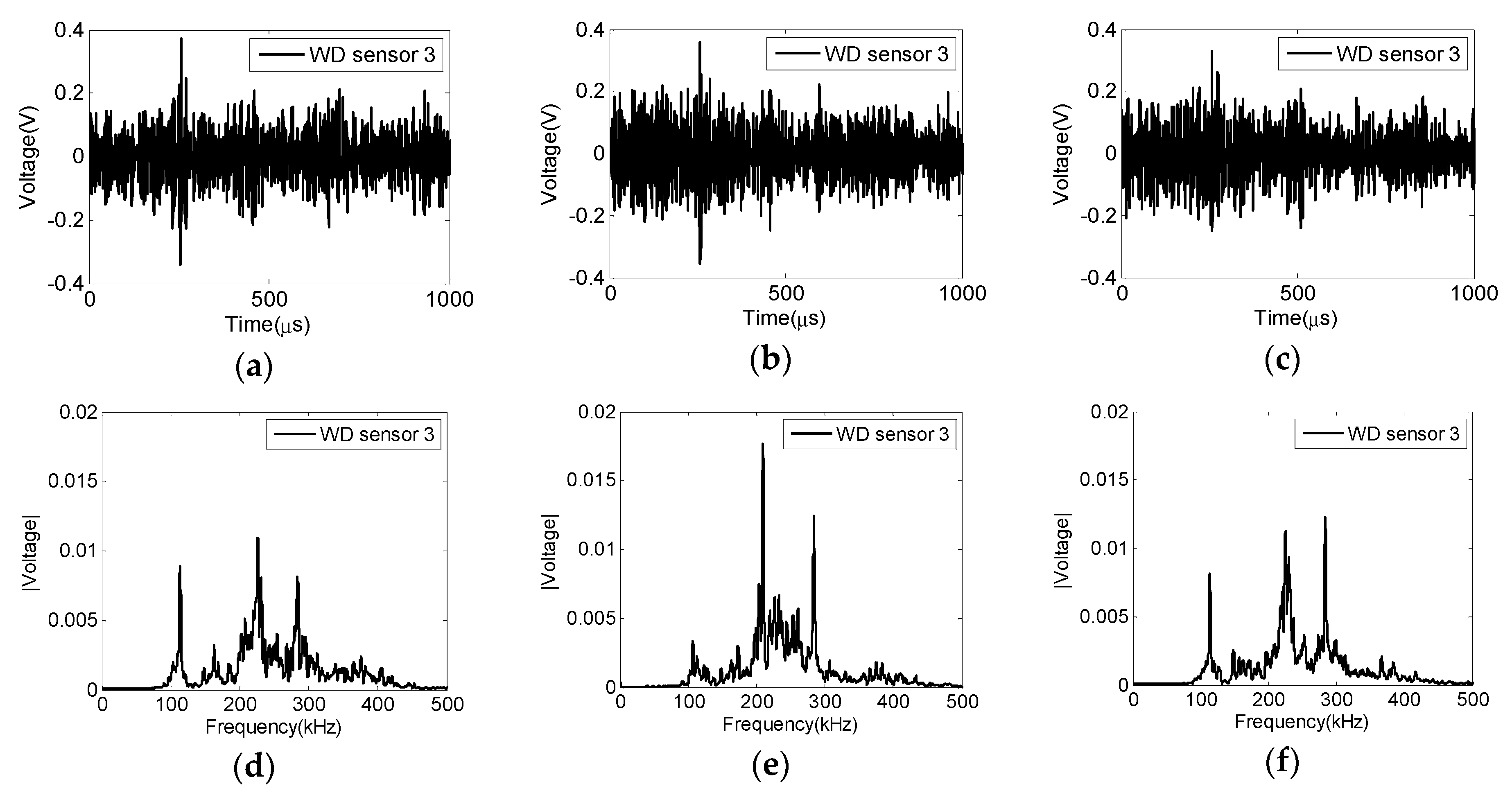
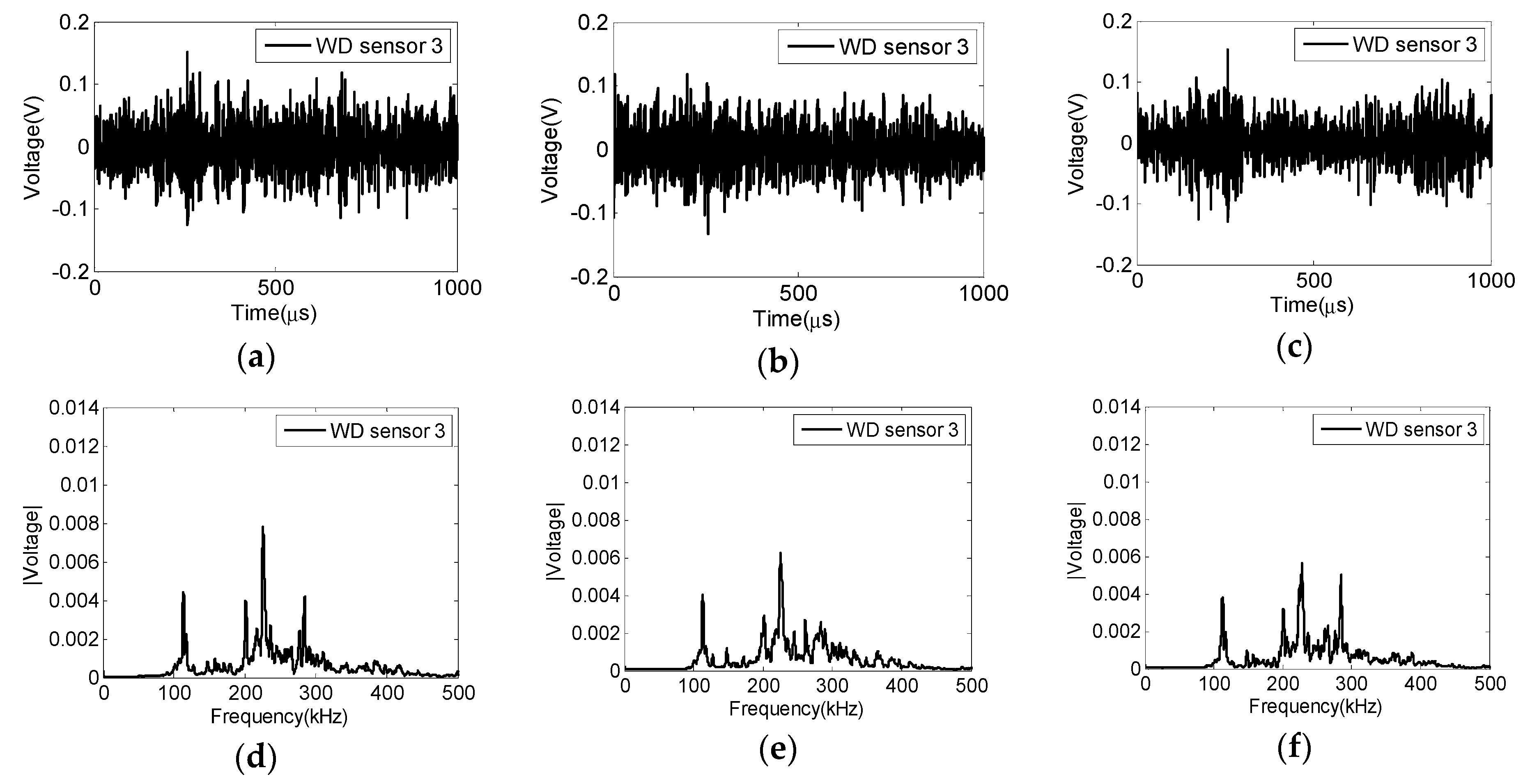
Figure 14 and Figure 15 show time histories and frequency spectra of six examples of continuous emission signals detected by sensor 3 near the peak load. There is a distinct frequency near 200 kHz. Typical mechanical friction sources generate AE signals below 100 kHz [50,51,52]. The increase in the frequency features (e.g., peak frequency, frequency centroid) can be considered as the initiation of plastic deformation if the sensors are positioned in proximity to the location of crack growth. It is important to emphasize that high-frequency signals are more attenuative than low-frequency signals with the increase of the distance between the sensor and the source; therefore, the attenuation characteristics should be considered if the sensor is placed further from the source implemented in this study.
5.3. The Comparison of Burst and Continuous AE Signals
A distinct difference between the frequency spectra of burst and continuous AE signals is observed as shown in Figure 16. The spectrograms are obtained using the complex Morlet Wavelet transform, which gives the best resolution in time and frequency [53,54]. While the main AE energy is in the frequency bandwidth of 100–150 kHz for the burst signal, it shifts to 200–250 kHz for continuous emission. Examples of burst and continuous AE signals are selected, and their AE characteristics (including peak frequency and frequency centroid) are extracted, as shown in Figure 17. In this figure, the weighted arithmetic average of the burst and continuous signals recorded at different fatigue cycles is presented. For continuous signals, about 100,000 AE hits recorded by channel 3 (located across notch tip), which occur near maximum loading are selected; the AE events located by three WD sensors during each day are selected as the statistical samples for burst signals. In general, the burst signals have lower peak frequency and frequency centroid than the continuous signals (see in Figure 17), which is consistent with the results in literature [55]. The AE amplitude does not indicate any distinct difference to identify two signal types. The other time domain features, such as duration and rise time, cannot be applied to continuous type signals. Thus, features in the frequency domain are needed to separate the AE source mechanisms.
5.4. Performance of Lead Zirconate Titanate (PZT) Wafer Sensor in the AE Mode
In order to evaluate the performance of PZT wafer sensors as AE sensors, their waveforms due to PLB simulation and fatigue crack, and the ability to detect the fatigue crack growth are compared with the performance of a Nano 30 sensor. The sources of AE signals compared in this section are verified by the triangulation array of WD sensors, as shown Figure 18. The red dots represent the AE events located by three WD sensors when PLB simulation (Figure 18a) is performed and fatigue crack growth (Figure 18b) occurs. The wave velocity is selected similar to the previous section as 3000 m/s. AE signals detected by the Nano 30 sensor and PZT wafer sensors at the same times of the AE events shown in Figure 18 are further analyzed.
Signal denoising is applied to improve the signal to noise ratio of PZT wafer sensors. The de-noising function is a one-dimensional wavelet function to find the lowest wavelet coefficients, which typically represent noise. Symlets 5 is selected as the orthogonal wavelet and five levels of decomposition are implemented. After wavelet coefficients below a pre-defined fixed threshold (value of 2.5125 selected in this study) are removed from the dataset, signals are reconstructed using an inverse wavelet transform. It is important to identify that the signal denoising process does not influence the major signal frequencies. Figure 19 shows the frequency spectra of pre-trigger and burst signal regions of piezoelectric wafer sensors under the PLB simulations. The electronic noise in the pre-trigger region has peak frequency near 100 kHz. The burst signal has frequencies near 200 kHz–400 kHz. Figure 20 compares the denoised and original signals. It is clearly shown that the denoising process increased the signal to noise ratio while preserving the major frequency components of the burst signal. The RMS-type features calculations in time and frequency domains in a short window could be used to avoid the influence of reflections to the AE features [56].
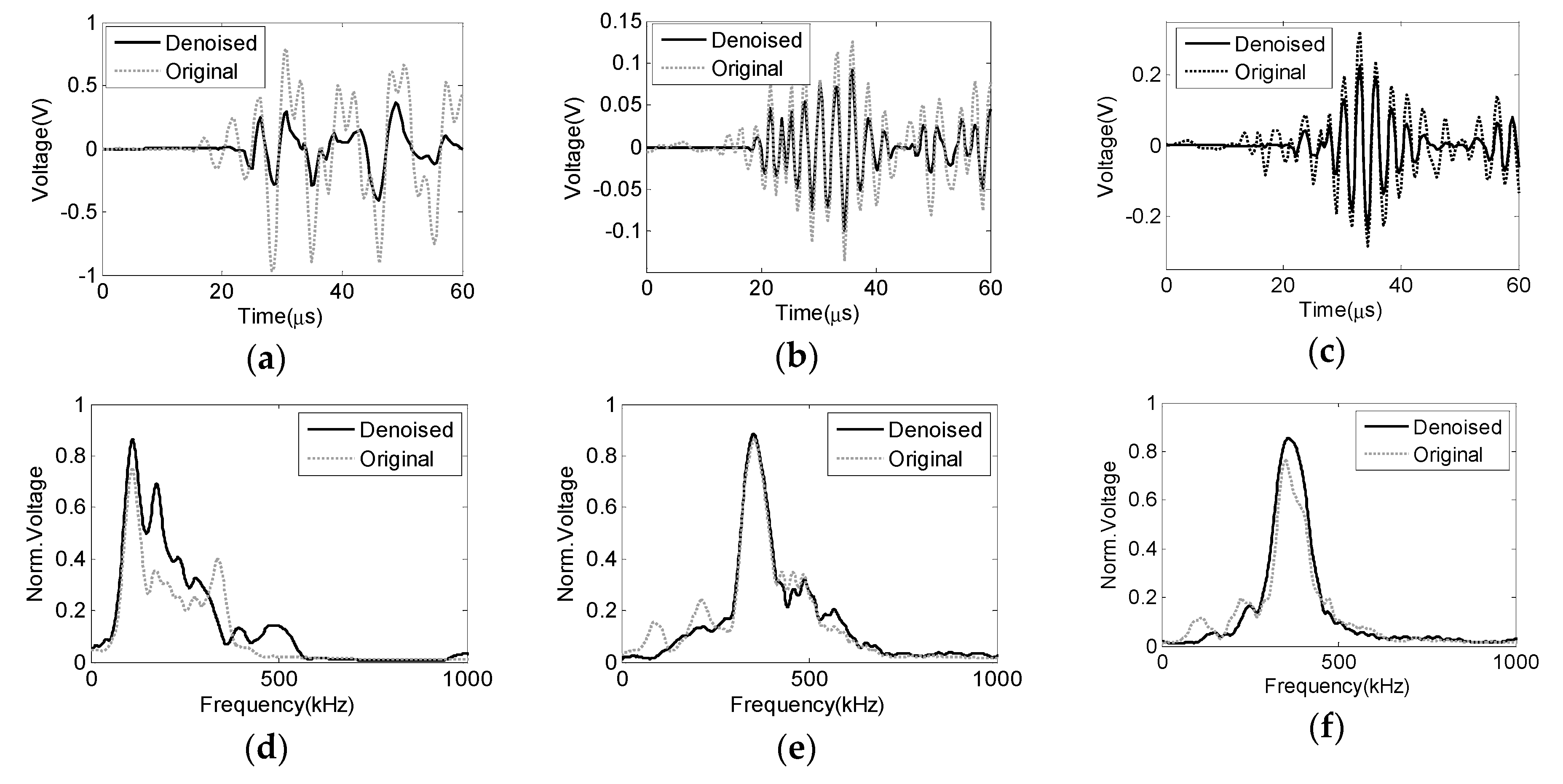
The denoising process has been applied to all the waveforms obtained by PLB simulations and fatigue testing. Figure 21 shows the time histories and frequency spectra of signals from Nano 30 and two PZT wafers obtained by PLB simulations. A windowed section of complete time histories is shown in Figure 22. While the AE source is the same and the sensors’ locations are similar, the responses of Nano 30 and PZT wafer sensors are different due to different transfer functions. The PZT wafer sensors have lower amplitude due to its relatively small size. Additionally, they exhibit a lower quality factor (i.e., higher damping) with lower ringing time than the Nano 30 sensor.
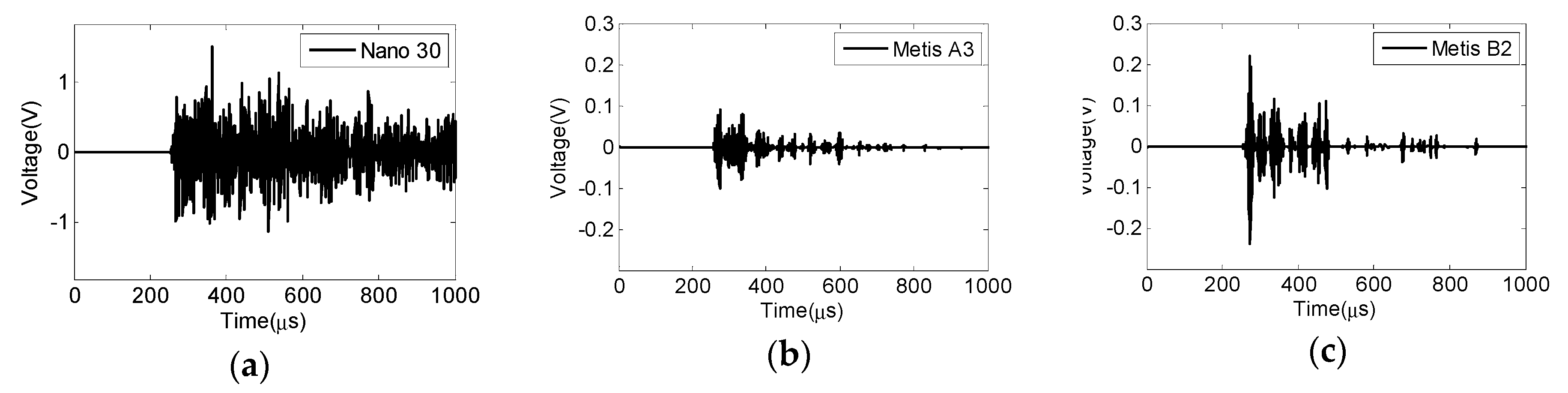
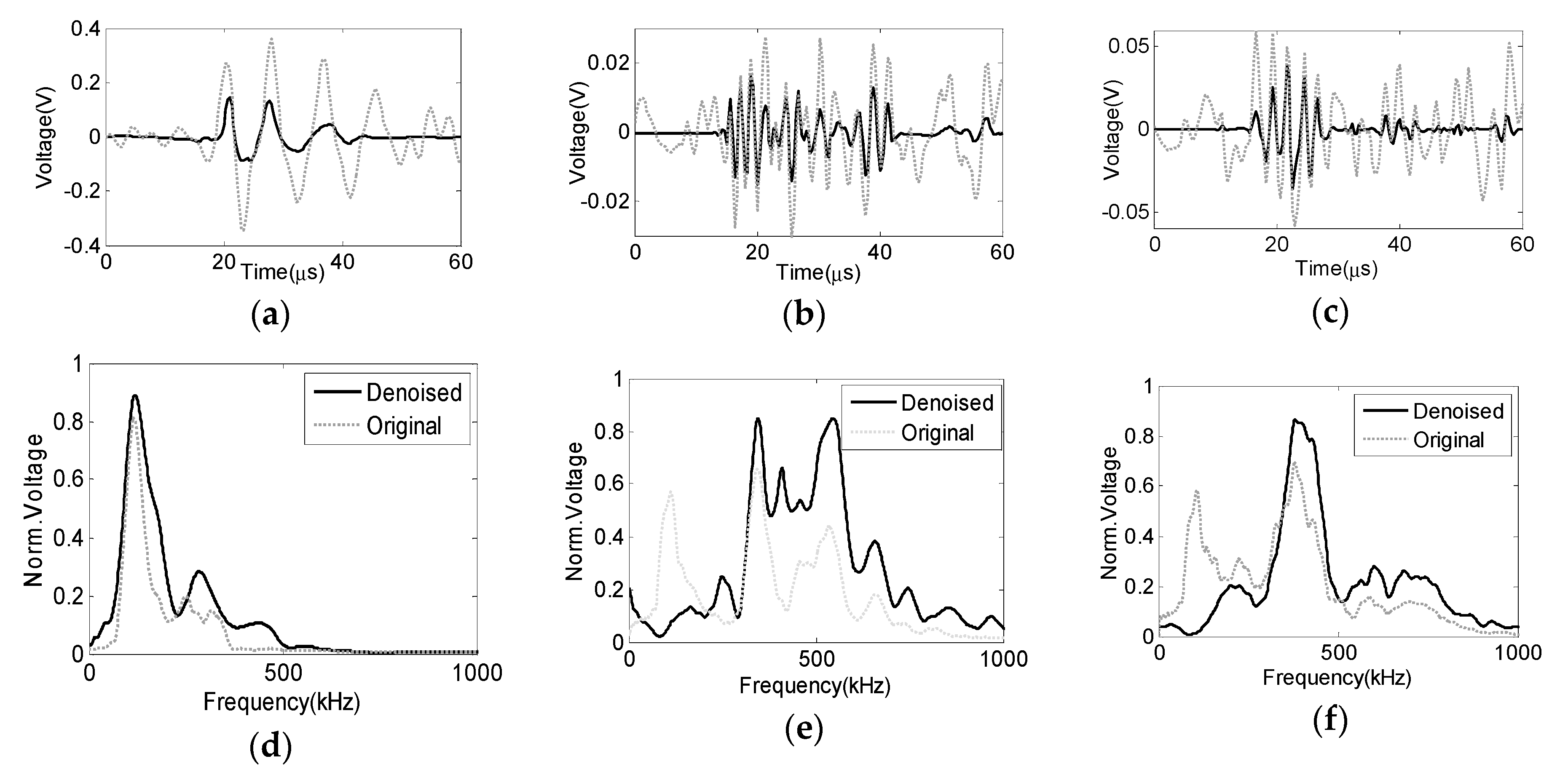
Figure 23 compares the waveforms of two sensor types detected during the fatigue experiment, and the selected AE event occurred near 400,000 cycles. Similar to PLB simulations, the amplitudes of PZT wafer sensors are lower than the amplitude of Nano 30. It is interesting to note that the waveforms and frequency distributions of AE signals due to fatigue crack growth are similar to PLB simulations, as shown in Figure 22, while the amplitude of the fatigue crack signal is about ten times smaller than the amplitude of PLB signal. This indicates the difference of energy levels of two source mechanisms with similar frequency spectrum.
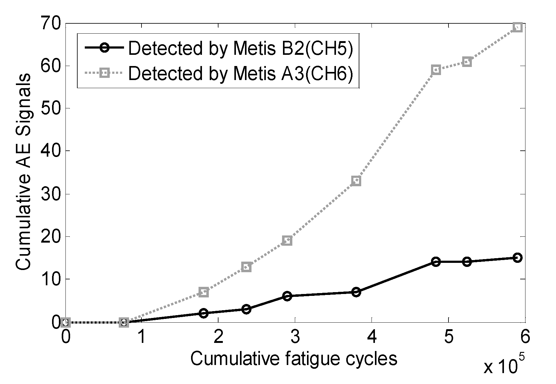
Based on the simulations and fatigue experiments, it is concluded that new piezoelectric sensor array can be utilized as an AE sensor. While their sensitivities are lower than bulky commercial AE sensors, they can be placed in proximity to crack locations inside the spline section of the gearbox, which eliminates the transmission loss of signal passing through all the layers of the gearbox components. The cumulative AE signals detected by piezoelectric wafer sensors near maximum loading with amplitude greater than 52 dB (above electronic noise level) are shown in Figure 24. The piezoelectric wafer sensors detect crack growth behavior similar to WD sensors, as shown in Figure 9a.
6. Conclusions
The detection of a fatigue crack in the idealized spline component of a gearbox using the AE method is presented in this paper. The crack length reached is about 7 mm in an angled direction at 590,211 cycles, which agrees with the numerical model. A detailed waveform analysis indicates that the plastic deformation and the crack jump have two distinct AE signatures in the forms of continuous emission and burst emission, respectively. Frequency domain features play significant roles in separating damage modes in complex metallic structures. A new piezoelectric sensor array is introduced with the intention of placing them in proximity to potential crack locations. While the sensors have low sensitivity compared to conventional piezoelectric AE sensors due to their relatively small size, they can detect the major crack growth events. As the sensor array can be placed inside the gearbox, the propagation path and the signal loss will not affect the signal signature and energy as compared to conventional AE sensors placed on the gearbox housing. The research will continue by adapting the AE patterns of two damage modes to the AE data recorded from the realistic test stand at the NAVAIR facility.
Acknowledgments
This material is based upon work supported by the U.S. Naval Air Systems Command (NAVAIR) under contract No. N68335-13-C-0417 entitled “Hybrid State-Detection System for Gearbox Components” awarded to the Metis Design Corporation. The authors would like to thank Seth Kessler and Gregory James for their inputs on the design of the test specimen. We acknowledge Daniel P. Bailey for detailed editing of the abstract and discussion of the manuscript. Any opinions, findings, and conclusions or recommendations expressed in this material are those of the authors and do not necessarily reflect the views of NAVAIR.
Author Contributions
Lu Zhang and Didem Ozevin conducted the experiments and analyzed the data. Lu Zhang also conducted the literature survey and wrote the background literature. William Hardman and Alan Timmons performed the Franc3D simulations and provided feedback on fatigue experiments and data processing.
Conflicts of Interest
The authors declare no conflict of interest.
References
- Sinha, P.; Bhattacharyya, S. Failure investigation of spline-shaft of an under slung crane. J. Fail. Anal. Prev. 2013, 13, 601–606. [Google Scholar] [CrossRef]
- Yu, Z.; Xu, X. Failure analysis of a diesel engine crankshaft. Eng. Fail. Anal. 2005, 12, 487–495. [Google Scholar] [CrossRef]
- Reuben, L.C.K.; Mba, D. Bearing time-to-failure estimation using spectral analysis features. Struct. Health Monit. 2014, 13, 219–230. [Google Scholar] [CrossRef]
- Hussain, S.; Gabbar, H.A. Gearbox fault detection using real coded genetic algorithm and novel shock response spectrum features extraction. J. Nondestruct. Eval. 2014, 33, 111–123. [Google Scholar] [CrossRef]
- Lin, S.T.; McFadden, P.D. Gear vibration analysis by B-spline wavelet-based linear wavelet transform. Mech. Syst. Signal Process. 1997, 11, 603–609. [Google Scholar] [CrossRef]
- Liu, B.; Riemenschneider, S.; Xu, Y. Gearbox Fault Diagnosis Using Empirical Mode Decomposition and Hilbert Spectrum. Mech. Syst. Signal Process. 2006, 20, 718–734. [Google Scholar] [CrossRef]
- Bonnardot, F.; El Badaoui, M.; Randall, R.B.; Danière, J.; Guillet, F. Use of the acceleration signal of a gearbox in order to perform angular resampling (with limited speed fluctuation). Mech. Syst. Signal Process. 2005, 19, 766–785. [Google Scholar] [CrossRef]
- Leturiondo, U.; Salgado, O.; Galar, D. Validation of a physics-based model of a rotating machine for synthetic data generation in hybrid diagnosis. Struct. Health Monit. 2016. [Google Scholar] [CrossRef]
- Pandya, Y.; Parey, A. Failure path based modified gear mesh stiffness for spur gear pair with tooth root crack. Eng. Fail. Anal. 2013, 27, 286–296. [Google Scholar] [CrossRef]
- Li, Z.; Yan, X.; Tian, Z.; Yuan, C.; Peng, Z.; Li, L. Blind vibration component separation and nonlinear feature extraction applied to the nonstationary vibration signals for the gearbox multi-fault diagnosis. Meas. J. Int. Meas. Confed. 2013, 46, 259–271. [Google Scholar] [CrossRef]
- Obuchowski, J.; Wylomanska, A.; Zimroz, R. Vibration Engineering and Technology of Machinery. Mech. Mach. Sci. 2015, 23, 401–410. [Google Scholar]
- Yunusa-Kaltungo, A.; Sinha, J.K.; Nembhard, A.D. A novel fault diagnosis technique for enhancing maintenance and reliability of rotating machines. Struct. Health Monit. 2015, 14, 1–18. [Google Scholar] [CrossRef]
- Elasha, F.; Greaves, M.; Mba, D.; Addali, A. Application of Acoustic Emission in Diagnostic of Bearing Faults within a Helicopter Gearbox. Procedia CIRP 2015, 38, 30–36. [Google Scholar] [CrossRef]
- Eftekharnejad, B.; Mba, D. Seeded fault detection on helical gears with acoustic emission. Appl. Acoust. 2009, 70, 547–555. [Google Scholar] [CrossRef]
- Gu, D.; Kim, J.; An, Y.; Choi, B. Detection of faults in gearboxes using acoustic emission signal. J. Mech. Sci. Technol. 2011, 25, 1279–1286. [Google Scholar] [CrossRef]
- Aggelis, D.; Shiotani, T.; Papacharalampopoulos, A.; Polyzos, D. The influence of propagation path on elastic waves as measured by acoustic emission parameters. Struct. Health Monit. 2012, 11, 359–366. [Google Scholar] [CrossRef]
- Khazaee, M.; Ahmadi, H.; Omid, M.; Moosavian, A.; Khazaee, M. Classifier fusion of vibration and acoustic signals for fault diagnosis and classification of planetary gears based on Dempster-Shafer evidence theory. Proc. Inst. Mech. Eng. Part E 2014, 228, 21–32. [Google Scholar] [CrossRef]
- Li, C.; Sanchez, R.-V.; Zurita, G.; Cerrada, M.; Cabrera, D.; Vásquez, R.E. Gearbox fault diagnosis based on deep random forest fusion of acoustic and vibratory signals. Mech. Syst. Signal Process. 2016, 76–77, 283–293. [Google Scholar] [CrossRef]
- Loutas, T.H.; Roulias, D.; Pauly, E.; Kostopoulos, V. The combined use of vibration, acoustic emission and oil debris on-line monitoring towards a more effective condition monitoring of rotating machinery. Mech. Syst. Signal Process. 2011, 25, 1339–1352. [Google Scholar] [CrossRef]
- Qu, Y.; He, D.; Yoon, J.; Van Hecke, B.; Bechhoefer, E.; Zhu, J. Gearbox tooth cut fault diagnostics using acoustic emission and vibration sensors—A comparative study. Sensors 2014, 14, 1372–1393. [Google Scholar] [CrossRef] [PubMed]
- Rezaei, A.; Dadouche, A. Development of a turbojet engine gearbox test rig for prognostics and health management. Mech. Syst. Signal Process. 2012, 33, 299–311. [Google Scholar] [CrossRef]
- Al-Ghamd, A.M.; Mba, D. A comparative experimental study on the use of acoustic emission and vibration analysis for bearing defect identification and estimation of defect size. Mech. Syst. Signal Process. 2006, 20, 1537–1571. [Google Scholar] [CrossRef]
- Bigus, G.A.; Travkin, A.A. An evaluation of the flaw-detection characteristics for the detection of fatigue cracks by the acoustic-emission method in samples made of steel 20 that have a cast structure. Russ. J. Nondestruct. Test. 2015, 51, 32–38. [Google Scholar] [CrossRef]
- Yu, J.G.; Ziehl, P. Stable and unstable fatigue prediction for A572 structural steel using acoustic emission. J. Constr. Steel Res. 2012, 77, 173–179. [Google Scholar] [CrossRef]
- Rastegaev, I.; Danyuk, A.; Afanas’yev, M.; Merson, D.; Berto, F.; Vinogradov, A. Acoustic emission assessment of impending fracture in a cyclically loading structural steel. Metals 2016, 6, 266. [Google Scholar] [CrossRef]
- Huang, M.; Jiang, L.; Liaw, P.K.; Brooks, C.R.; Seeley, R.; Klarstrom, L.D. Using Acoustic Emission in Fatigue and Fracture Materials Research. Mater. Res. 1998, 50, 1–13. [Google Scholar]
- Burridge, R.; Knopoff, L. Body Force Equivalents for Seismic Dislocations. Seismol. Res. Lett. 2003, 74, 154–162. [Google Scholar] [CrossRef]
- Ohtsu, M. Acoustic emission theory for moment tensor analysis. J. Res. Nondestruct. Eval. 1995, 169–184. [Google Scholar] [CrossRef]
- Ohtsu, M. Source kinematics of acoustic emission based on a moment tensor. NDT Int. 1989, 22, 14–20. [Google Scholar]
- Ohtsu, M.; Ono, K. The generalized theory and source representations of acoustic emission. J. Acoust. Emiss. 1986, 5, 124–133. [Google Scholar]
- Healy, D.; Jones, R.R.; Holdsworth, R.E. Three-dimensional brittle shear fracturing by tensile crack interaction. Nature 2006, 439, 64–67. [Google Scholar] [CrossRef] [PubMed]
- Kao, C.-S.; Carvalho, F.C.S.; Labuz, J.F. Micromechanisms of fracture from acoustic emission. Int. J. Rock Mech. Min. Sci. 2011, 48, 666–673. [Google Scholar] [CrossRef]
- Ohira, T.; Pao, Y. Quantitative characterization of microcracking in A533B steel by acoustic emission. Metall. Trans. A 1989, 20, 1105–1114. [Google Scholar] [CrossRef]
- Ohno, K.; Uji, K.; Ueno, A.; Ohtsu, M. Fracture process zone in notched concrete beam under three-point bending by acoustic emission. Constr. Build. Mater. 2014, 67, 139–145. [Google Scholar] [CrossRef]
- Sause, M.G.R.; Horn, S. Simulation of Acoustic Emission in Planar Carbon Fiber Reinforced Plastic Specimens. J. Nondestruct. Eval. 2010, 29, 123–142. [Google Scholar] [CrossRef]
- Yu, J.; Ziehl, P.; Matta, F.; Pollock, A. Acoustic emission detection of fatigue damage in cruciform welded joints. J. Constr. Steel Res. 2013, 86, 85–91. [Google Scholar] [CrossRef]
- Li, R.; Seçkiner, S.U.; He, D.; Bechhoefer, E.; Menon, P. Gear fault location detection for split torque gearbox using AE sensors. IEEE Trans. Syst. Man Cybern. Part C 2012, 42, 1308–1317. [Google Scholar] [CrossRef]
- Poddar, B.; Giurgiutiu, V. Detectability of Crack Lengths from Acoustic Emissions Using Physics of Wave Propagation in Plate Structures. J. Nondestruct. Eval. 2017, 36, 41. [Google Scholar] [CrossRef]
- Caesarendra, W.; Kosasih, B.; Tieu, A.K.; Zhu, H.; Moodie, C.A.S.; Zhu, Q. Acoustic emission-based condition monitoring methods: Review and application for low speed slew bearing. Mech. Syst. Signal Process. 2015, 72, 134–159. [Google Scholar] [CrossRef]
- Li, R.; He, D. Rotational machine health monitoring and fault detection using EMD-based acoustic emission feature quantification. IEEE Trans. Instrum. Meas. 2012, 61, 990–1001. [Google Scholar] [CrossRef]
- Soua, S.; Van Lieshout, P.; Perera, A.; Gan, T.H.; Bridge, B. Determination of the combined vibrational and acoustic emission signature of a wind turbine gearbox and generator shaft in service as a pre-requisite for effective condition monitoring. Renew. Energy 2013, 51, 175–181. [Google Scholar] [CrossRef]
- Siracusano, G.; Lamonaca, F.; Tomasello, R.; Garescì, F.; Corte, A.L.; Carnì, D.L.; Carpentieri, M.; Grimaldi, D.; Finocchio, G. A framework for the damage evaluation of acoustic emission signals through Hilbert-Huang transform. Mech. Syst. Signal Process. 2016, 75, 109–122. [Google Scholar] [CrossRef]
- Raja Hamzah, R.I.; Mba, D. The influence of operating condition on acoustic emission (AE) generation during meshing of helical and spur gear. Tribol. Int. 2009, 42, 3–14. [Google Scholar] [CrossRef]
- Loutas, T.H.; Sotiriades, G.; Kalaitzoglou, I.; Kostopoulos, V. Condition monitoring of a single-stage gearbox with artificially induced gear cracks utilizing on-line vibration and acoustic emission measurements. Appl. Acoust. 2009, 70, 1148–1159. [Google Scholar] [CrossRef]
- Tan, C.K.; Mba, D. Identification of the acoustic emission source during a comparative study on diagnosis of a spur gearbox. Tribol. Int. 2005, 38, 469–480. [Google Scholar] [CrossRef]
- Tan, C.K.; Mba, D. Limitation of acoustic emission for identifying seeded defects in gearboxes. J. Nondestruct. Eval. 2005, 24, 11–28. [Google Scholar] [CrossRef]
- Toutountzakis, T.; Mba, D. Observations of acoustic emission activity during gear defect diagnosis. NDT E Int. 2003, 36, 471–477. [Google Scholar] [CrossRef]
- Ozevin, D.; Cox, J.; Hardman, W.; Kessler, S.; Timmons, A. Fatigue Crack Detection at Gearbox Spline Component using Acoustic Emission Method. In Proceedings of the Annual Conference of the Prognostics and Health Management Society, Forth Worth, TX, USA, 29 September–2 October 2014. [Google Scholar]
- Giurgiutiu, V. Structural Health Monitoring: With Piezoelectric Wafer Active Sensors; Academic Press: Cambridge, MA, USA, 2007. [Google Scholar]
- Boyun, G.; Song, S.; Ghalambor, A.; Lin, T.R. Offshore Pipelines Design, Installation, and Maintenance; Gulf Professional Publishing: Houston, TX, USA, 2014; p. 383. [Google Scholar]
- Hase, A.; Mishina, H.; Wada, M. Correlation between features of acoustic emission signals and mechanical wear mechanisms. Wear 2012, 292–293, 144–150. [Google Scholar] [CrossRef]
- Rogers, L.M. The application of vibration signature analysis and acoustic emission source location to on-line condition monitoring of anti-friction bearings. Tribol. Int. 1979, 12, 51–58. [Google Scholar] [CrossRef]
- Lin, J.; Qu, L. Feature Extraction Based on Morlet Wavelet and Its Application for Mechanical Fault Diagnosis. J. Sound Vib. 2000, 234, 135–148. [Google Scholar] [CrossRef]
- Mostavi, A.; Kamali, N.; Tehrani, N.; Chi, S.W.; Ozevin, D.; Indacochea, J.E. Wavelet based harmonics decomposition of ultrasonic signal in assessment of plastic strain in aluminum. Meas. J. Int. Meas. Confed. 2017, 106, 66–78. [Google Scholar] [CrossRef]
- Pomponi, E.; Vinogradov, A. A real-time approach to acoustic emission clustering. Mech. Syst. Signal Process. 2013, 40, 791–804. [Google Scholar] [CrossRef]
- Martínez-Jequier, J.; Gallego, A.; Suárez, E.; Juanes, F.J.; Valea, Á. Real-time damage mechanisms assessment in CFRP samples via acoustic emission Lamb wave modal analysis. Composites Part B 2015, 68, 317–326. [Google Scholar] [CrossRef]
Figure 1.
The measurement chain of AE signals.

Figure 2.
The flattened spline section and dimensions (unit: mm).
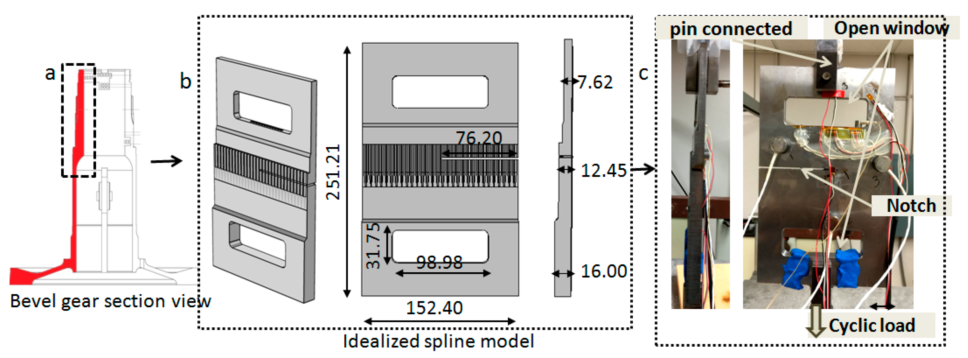
Figure 3.
The schematics of numerical models to study the influence of geometric details on AE signatures; (a) excitation and sensor; (b) simple model; and (c) complex model (unit: mm).
Figure 3.
The schematics of numerical models to study the influence of geometric details on AE signatures; (a) excitation and sensor; (b) simple model; and (c) complex model (unit: mm).
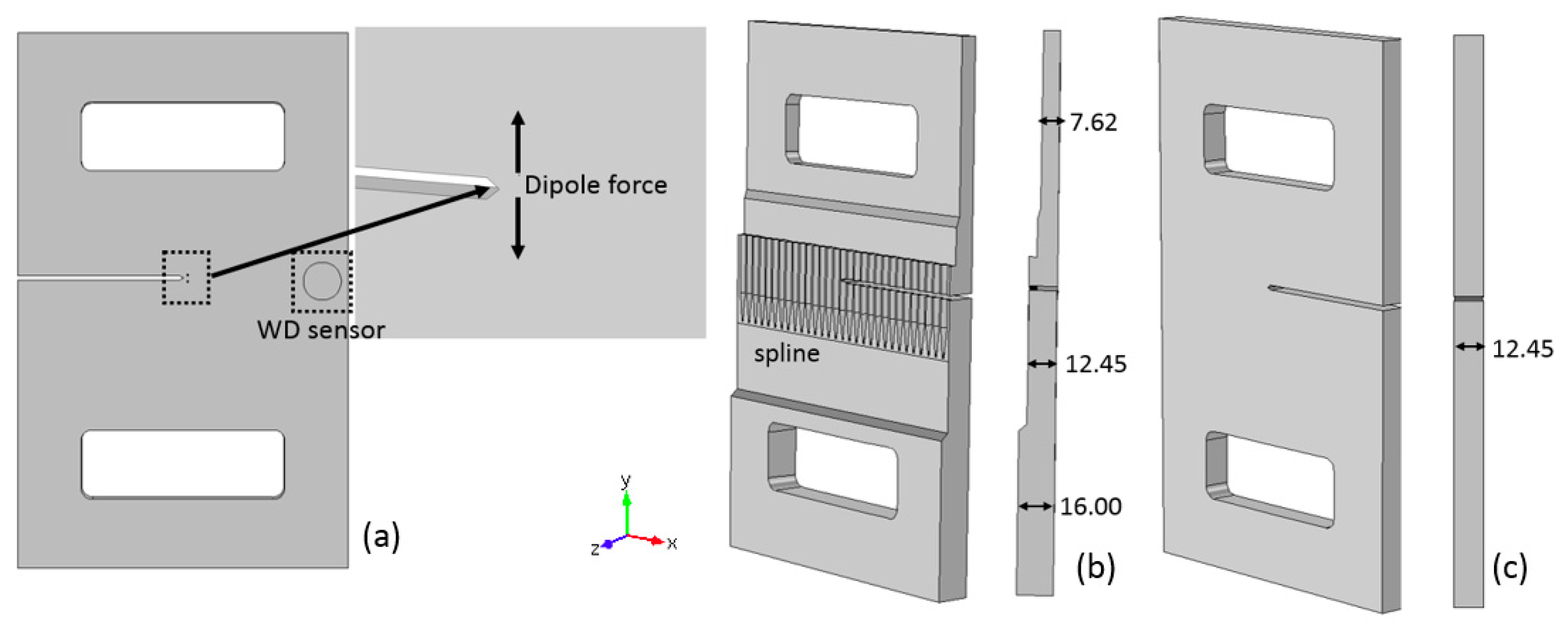
Figure 4.
The comparison of displacement responses in frequency domain, (a) z direction; (b) y direction; and (c) x direction.
Figure 4.
The comparison of displacement responses in frequency domain, (a) z direction; (b) y direction; and (c) x direction.

Figure 5.
The experimental setup, (a) data acquisition systems; (b) the sensor positions; and (c) the sensors on the window section.
Figure 5.
The experimental setup, (a) data acquisition systems; (b) the sensor positions; and (c) the sensors on the window section.

Figure 6.
The Franc3D model and the predicted crack growth rate (a) sample model; (b) mesh around the notch tip, crack direction in the model and experiment; (c–e) crack lines along different crack surfaces and corresponding SIFs.
Figure 6.
The Franc3D model and the predicted crack growth rate (a) sample model; (b) mesh around the notch tip, crack direction in the model and experiment; (c–e) crack lines along different crack surfaces and corresponding SIFs.
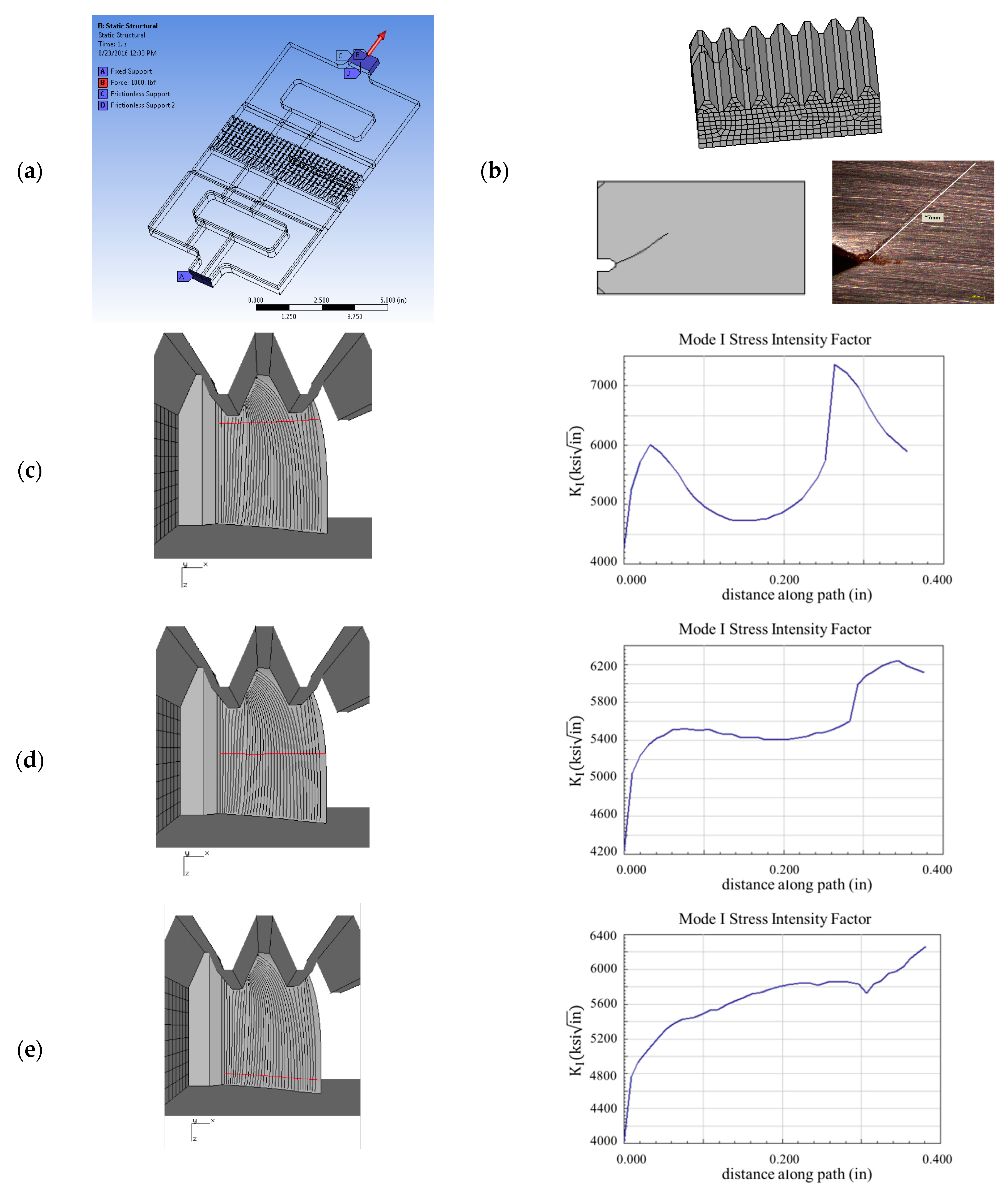
Figure 7.
The AE event locations detected during the fatigue tests from day 1 to day 8: (a) day 1; (b) day 2; (c) day 3; (d) day 4; (e) day 5; (f) day 6; (g) day 7; and (h) day 8.
Figure 7.
The AE event locations detected during the fatigue tests from day 1 to day 8: (a) day 1; (b) day 2; (c) day 3; (d) day 4; (e) day 5; (f) day 6; (g) day 7; and (h) day 8.
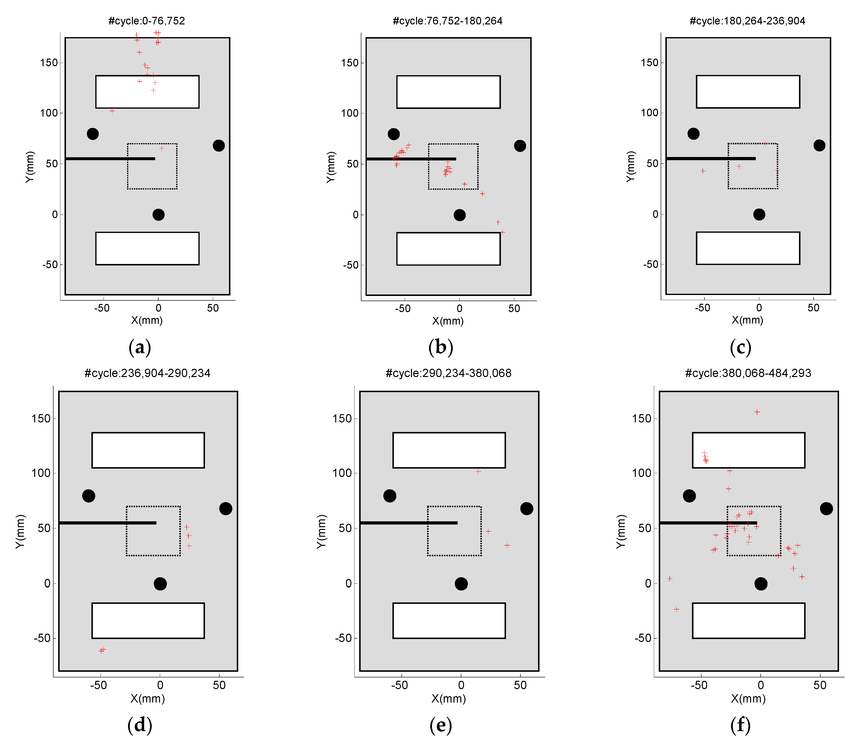

Figure 8.
The strain history versus cumulative AE events; (a) strain gauge 1; and (b) strain gauge 2.
Figure 8.
The strain history versus cumulative AE events; (a) strain gauge 1; and (b) strain gauge 2.

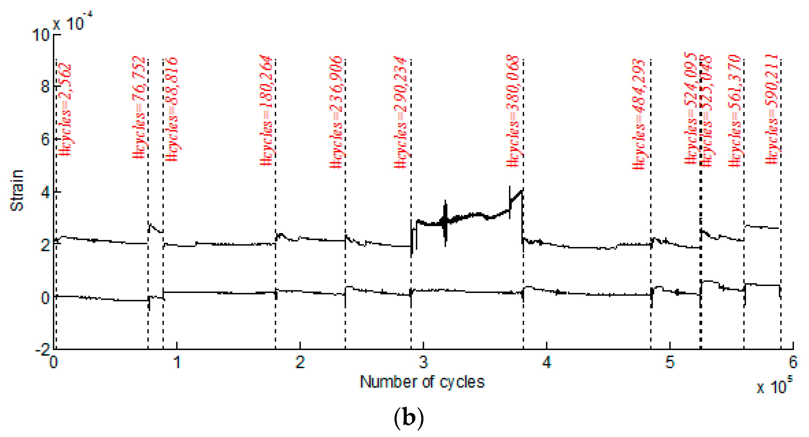
Figure 9.
(a) Cumulative AE events and fatigue cycles, microscopic image of crack growth; (b) back surface; (c) front surface; and (d) Sonoscan microscopic image.
Figure 9.
(a) Cumulative AE events and fatigue cycles, microscopic image of crack growth; (b) back surface; (c) front surface; and (d) Sonoscan microscopic image.

Figure 10.
Static finite element model with different crack lengths in the growth direction.

Figure 11.
The comparison of experimental and numerical strain history; (a) experimental measurement; and (b) numerical measurement.
Figure 11.
The comparison of experimental and numerical strain history; (a) experimental measurement; and (b) numerical measurement.

Figure 12.
Time domain histories and frequency spectra of the AE event detected by three WD sensors, and located near the notch tip at about 400,000 cycles, where (a,d) are from sensor 1; (b,e) are from sensor 2; and (c,f) are from sensor 3.
Figure 12.
Time domain histories and frequency spectra of the AE event detected by three WD sensors, and located near the notch tip at about 400,000 cycles, where (a,d) are from sensor 1; (b,e) are from sensor 2; and (c,f) are from sensor 3.
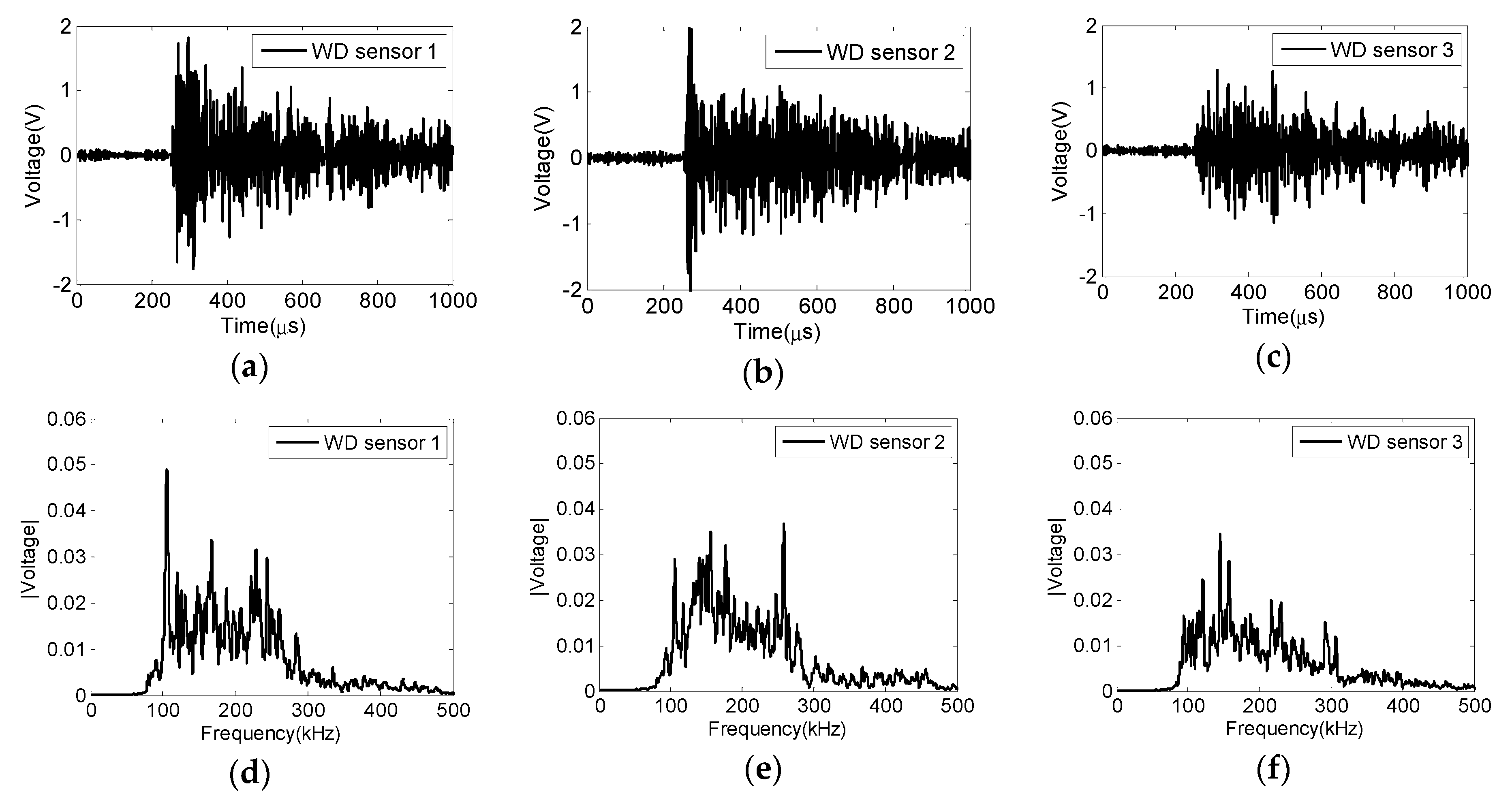
Figure 13.
The selected continuous emission recorded near peak load; (a) day 5, and (b) day 6.

Figure 14.
Examples of continuous AE signals and frequency spectra detected by sensor 3 for day 5 (290,234–380,068 cycles), where (a,d), (b,e), and (c,f) are from three different signals, respectively.
Figure 14.
Examples of continuous AE signals and frequency spectra detected by sensor 3 for day 5 (290,234–380,068 cycles), where (a,d), (b,e), and (c,f) are from three different signals, respectively.

Figure 15.
Examples of continuous AE signals and frequency spectra detected by sensor 3 for day 6 (380,068–484,293 cycles), where (a,d), (b,e), and (c,f) are from three different signals, respectively.
Figure 15.
Examples of continuous AE signals and frequency spectra detected by sensor 3 for day 6 (380,068–484,293 cycles), where (a,d), (b,e), and (c,f) are from three different signals, respectively.

Figure 16.
(a) The comparison of frequency spectra between burst type and continuous type signals; (b) spectrogram of burst type signal and (c) spectrogram of continuous type signal.
Figure 16.
(a) The comparison of frequency spectra between burst type and continuous type signals; (b) spectrogram of burst type signal and (c) spectrogram of continuous type signal.
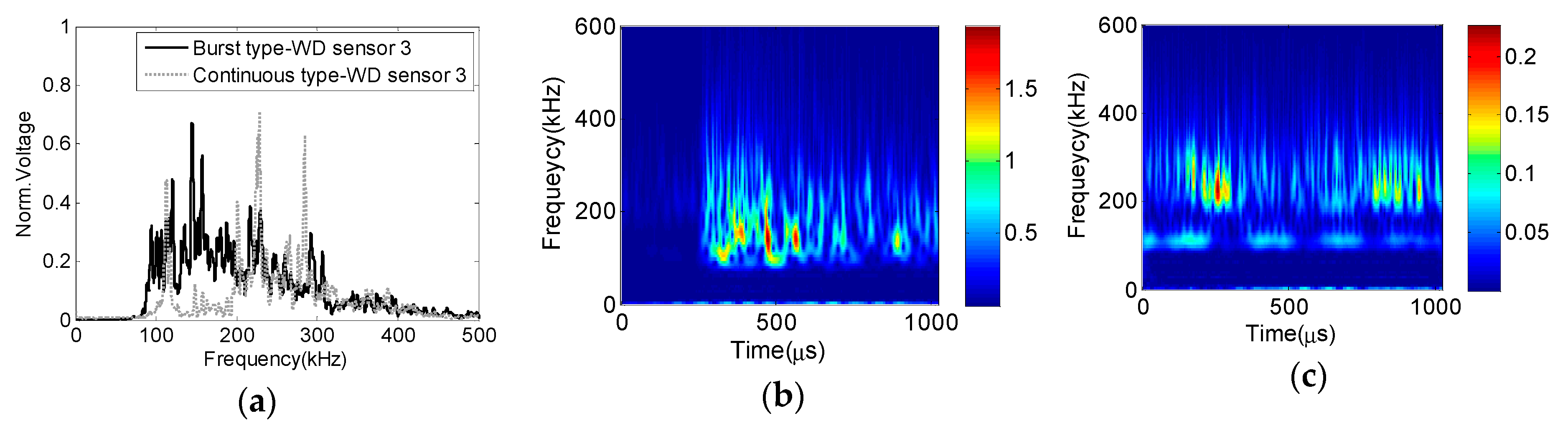
Figure 17.
The histogram of burst and continuous signals; (a) peak frequency, and (b) frequency centroid.
Figure 17.
The histogram of burst and continuous signals; (a) peak frequency, and (b) frequency centroid.
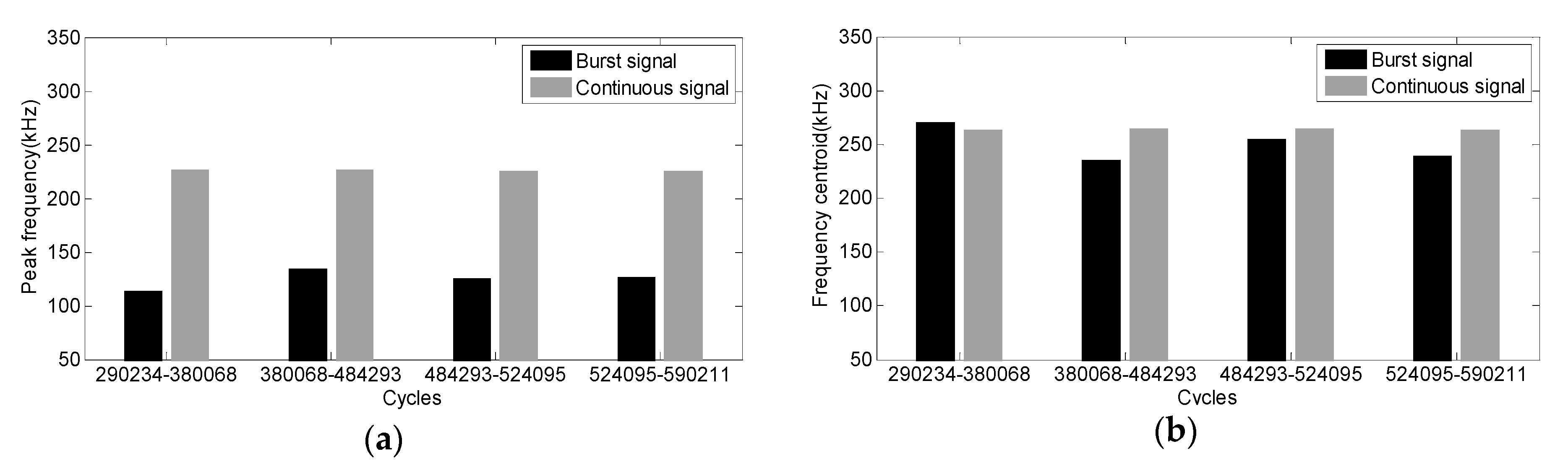
Figure 18.
The selected AE events near the notch tip detected by all the sensors; (a) an artificial event generated by PLB simulation; and (b) a real event generated by fatigue crack growth.
Figure 18.
The selected AE events near the notch tip detected by all the sensors; (a) an artificial event generated by PLB simulation; and (b) a real event generated by fatigue crack growth.
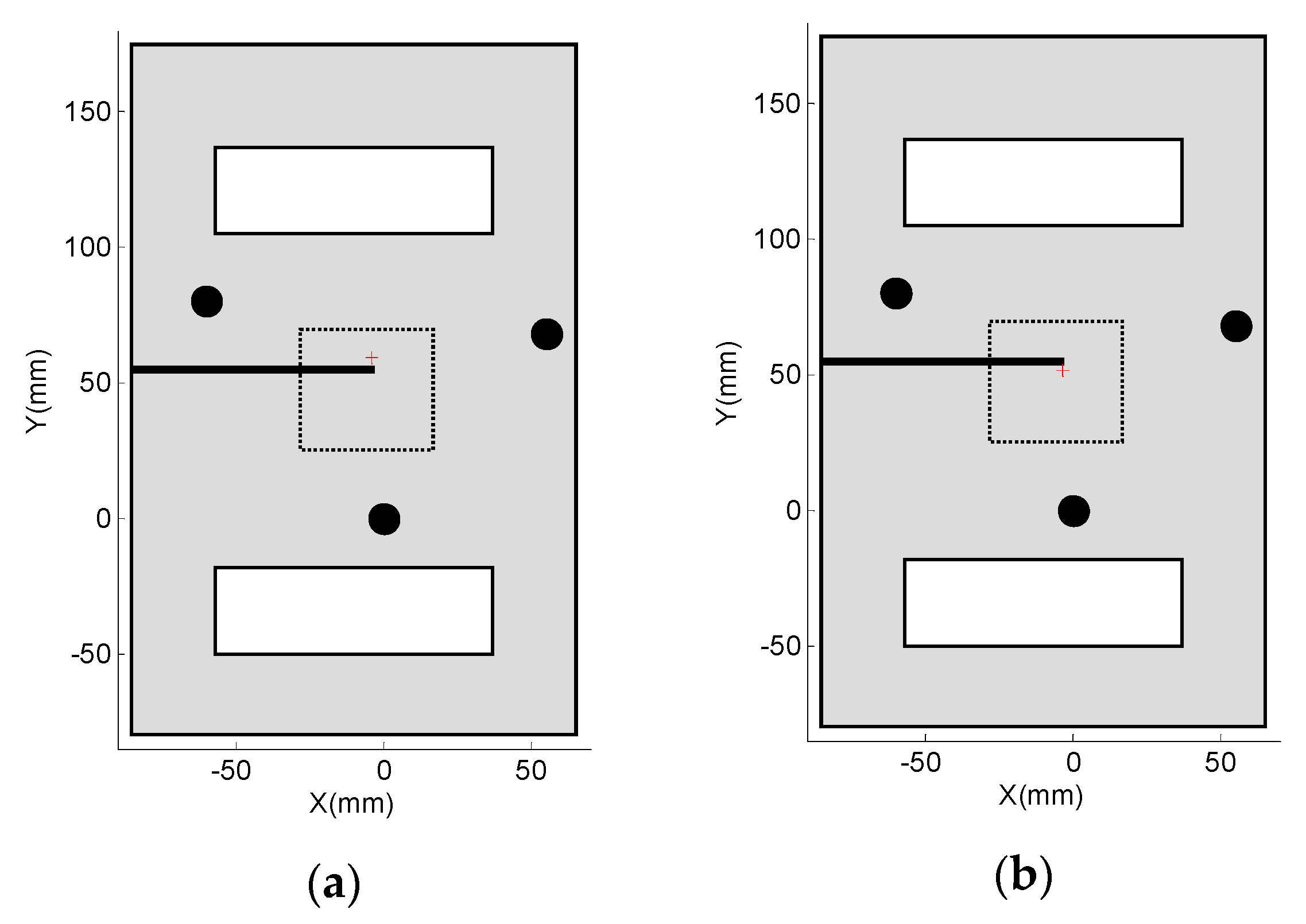
Figure 19.
Time and frequency domain response of pre-trigger and burst signal regions of PZT wafer sensors, where (a,c) are from Metis A3; and (b,d) are from Metis B2.
Figure 19.
Time and frequency domain response of pre-trigger and burst signal regions of PZT wafer sensors, where (a,c) are from Metis A3; and (b,d) are from Metis B2.
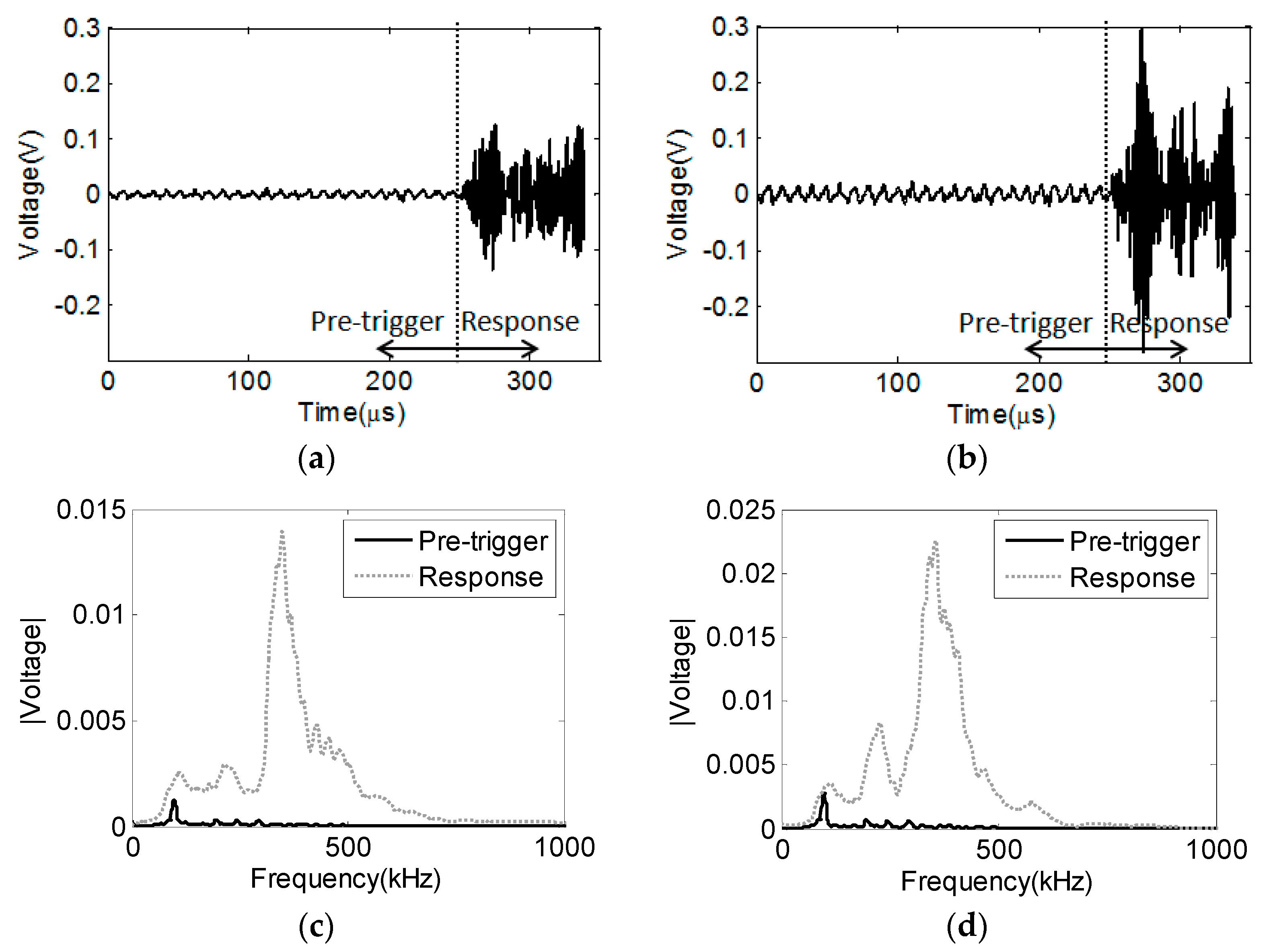
Figure 20.
The time and frequency domain responses of PZT wafer sensors generated by PLB simulation, where (a,c) are from Metis A3, and (b,d) are from Metis B2.
Figure 20.
The time and frequency domain responses of PZT wafer sensors generated by PLB simulation, where (a,c) are from Metis A3, and (b,d) are from Metis B2.
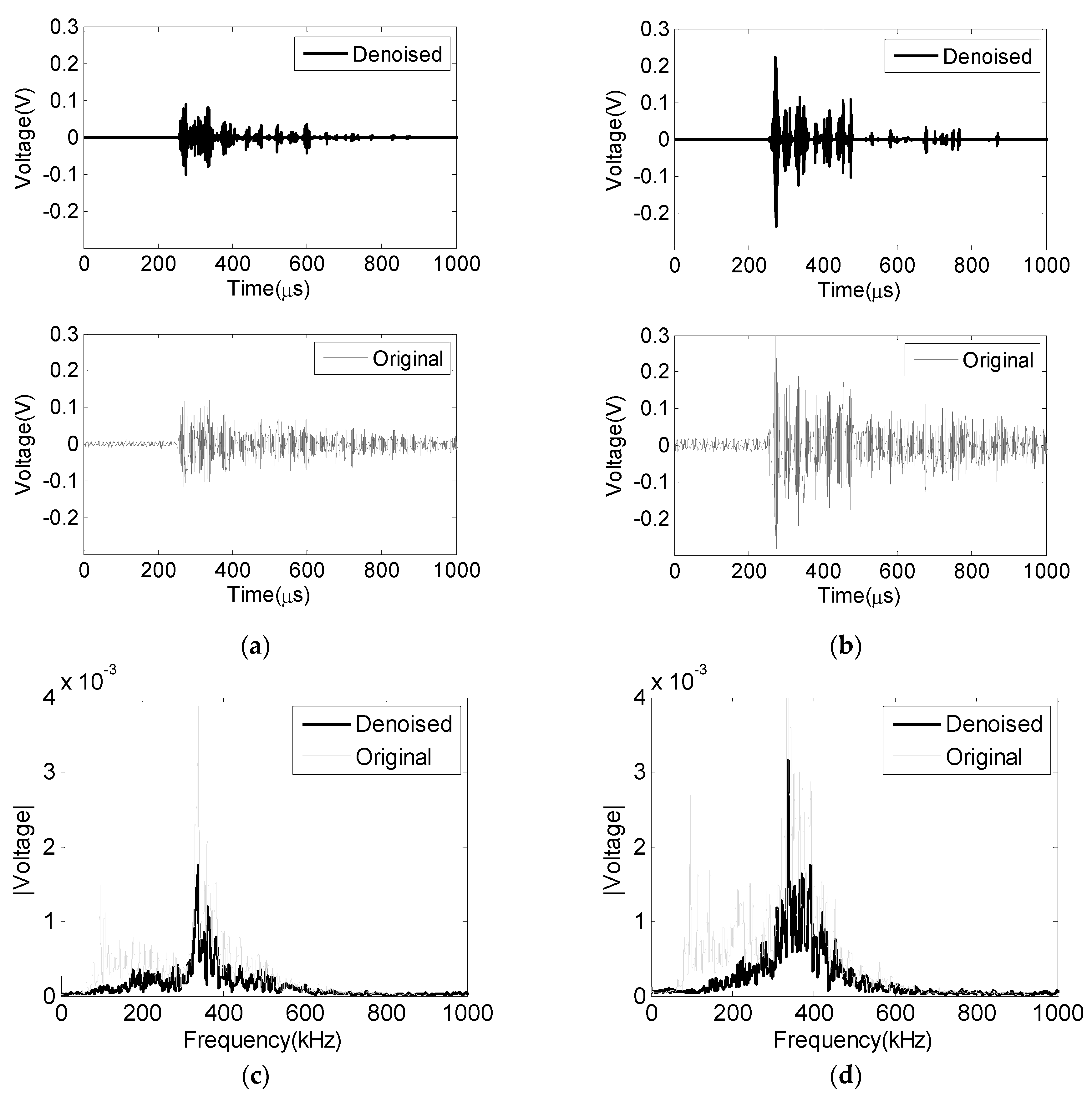
Figure 21.
Complete time history waveforms and their frequency spectra generated by PLB simulations, where (a,d) are from Nano 30; (b,e) are from Metis A3; and (c,f) are from Metis B2.
Figure 21.
Complete time history waveforms and their frequency spectra generated by PLB simulations, where (a,d) are from Nano 30; (b,e) are from Metis A3; and (c,f) are from Metis B2.

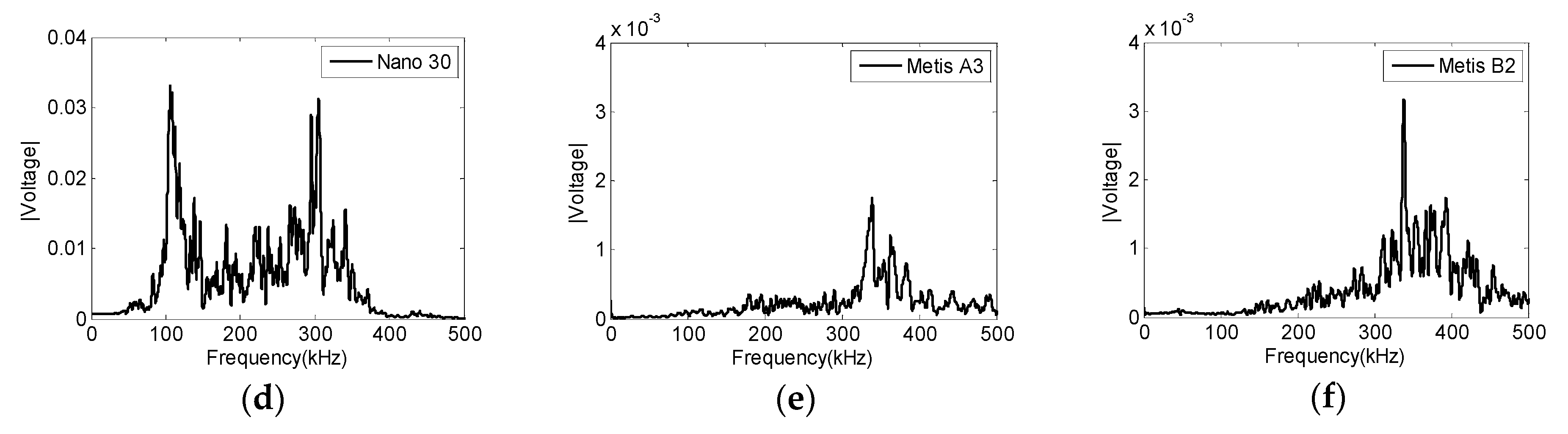
Figure 22.
Windowed time history waveforms and their frequency spectra generated by PLB simulations, where (a,d) are from Nano 30; (b,e) are from Metis A3; and (c,f) are from Metis B2.
Figure 22.
Windowed time history waveforms and their frequency spectra generated by PLB simulations, where (a,d) are from Nano 30; (b,e) are from Metis A3; and (c,f) are from Metis B2.

Figure 23.
Windowed time history waveforms and their frequency spectra generated by fatigue crack growth, where (a,d) are from Nano 30, (b,e) are from Metis A3, and (c,f) are from Metis B2.
Figure 23.
Windowed time history waveforms and their frequency spectra generated by fatigue crack growth, where (a,d) are from Nano 30, (b,e) are from Metis A3, and (c,f) are from Metis B2.

Figure 24.
Cumulative AE signals from Metis A3 and Metis B2 and fatigue cycles.
© 2017 by the authors. Licensee MDPI, Basel, Switzerland. This article is an open access article distributed under the terms and conditions of the Creative Commons Attribution (CC BY) license (http://creativecommons.org/licenses/by/4.0/).
Share and Cite
MDPI and ACS Style
Zhang, L.; Ozevin, D.; Hardman, W.; Timmons, A. Acoustic Emission Signatures of Fatigue Damage in Idealized Bevel Gear Spline for Localized Sensing. Metals 2017, 7, 242. https://doi.org/10.3390/met7070242
AMA Style
Zhang L, Ozevin D, Hardman W, Timmons A. Acoustic Emission Signatures of Fatigue Damage in Idealized Bevel Gear Spline for Localized Sensing. Metals. 2017; 7(7):242. https://doi.org/10.3390/met7070242
Chicago/Turabian StyleZhang, Lu, Didem Ozevin, William Hardman, and Alan Timmons. 2017. "Acoustic Emission Signatures of Fatigue Damage in Idealized Bevel Gear Spline for Localized Sensing" Metals 7, no. 7: 242. https://doi.org/10.3390/met7070242
Note that from the first issue of 2016, this journal uses article numbers instead of page numbers. See further details here.