NURBS-Based Collocation Methods for the Structural Analysis of Shells of Revolution

Abstract

In this work we present a collocation method for the structural analysis of shells of revolution based on Non-Uniform Rational B-Spline (NURBS) interpolation. The method is based on the strong formulation of the equilibrium equations according to Reissner-Mindlin theory, with Fourier series expansion of dependent variables, which makes the problem 1D. Several numerical tests validate convergence, accuracy, and robustness of the proposed methodology, and its feasibility as a tool for the analysis and design of complex shell structures.

1. Introduction

The application of differential quadrature or collocation methods for the solution of engineering boundary value problems dates back to the initial works by Bellmann and Casti [1,2], who are credited to have introduced the term differential quadrature operator, as the counterpart of quadrature operator for the approximation of a differential operator, i.e., the strong form of the equation; and having applied this strategy to first-order ordinary non-linear differential equations. The terminology of collocation method is, to the best of the authors’ knowledge, associated with the work by Petersen [3], and subsequently with the work by Karpilovskaya [4], Vainikko [5,6] and Kaspshitskaya [7]. The two methods share substantial similarities, namely the main idea of solving the strong form of the problem with a proper choice of discrete function spaces of approximation. By introducing a proper interpolation of the dependent variables, which is substituted in the governing differential equations, a linear set of equations for the unknown variables can be written by enforcing (i.e., collocating) the discretized form of the governing equations at a set of locations on the domain, known as collocation points.

The method appears to have gained more interest in the scientific research community in the last two decades, rather than immediately following the presentation in the scientific literature. Nowadays, there is discussion as to whether this methodology may become a valid and general purpose alternative to more established methods such as the finite element method [8]. Without trying to give a general answer to this question, and without trying to provide a detailed literary review of the many applications of the collocation or differential quadrature method in past works, the aim of the present communication is to present an innovative formulation of the collocation method for the analysis of shells of revolution based on Non Uniform Rational B-Spline (NURBS) functions.

The collocation method is ideal in application to structural theories and has found several instances in the scientific literature [9]. With reference to the analysis of shell structural elements, Mirfakhraei and Redekop [10] applied a Lagrangian differential quadrature method to the study of buckling phenomena of orthotropic thin shells of revolution; Wu et al [11,12] presented solutions to problems of axisymmetric bending of shells of revolution, introducing the so-called generalized differential quadrature rule. Viola and Artioli [13,14] and Artioli et al. [15,16] proposed a Lagrange differential quadrature solution for complex rotational shells with Fourier series expansion of dependent variables, both for the free vibration analysis, and for the static analysis of shells of revolution subject to unsymmetrical loading. The application of a collocation or differential quadrature method using Spline interpolants had been already proposed by Bellman and co-workers to solve general fourth-order differential equation problems [17], and later applied by Zhong and Guo [18,19] to static and buckling problems for Kirchhoff plates and to the non-linear free vibration analysis of straight Euler beams, respectively. Dade Huang proposed a Spline based collocation method for laminated plates and shells [20], while Viswanathan introduced the collocation method with Spline basis function in application to shear deformable laminated plates and shells [21,22,23].

The recent exponential growth of the isogeometric analysis [24,25,26,27,28,29] has raised attention on collocation methods based on NURBS and/or T-Splines trial functions. Given their higher-order smoothness and their favorable approximation properties, NURBS basis functions constitute an efficient interpolation tool for collocating differential operators, i.e., for the approximation of the strong formulation of PDEs; furthermore they apply even to irregular or complex geometric domains. The newly developed IGA Collocation methods [8,30,31,32,33], set in the realm of weighted residuals [35], have been applied to a variety of solid, structural mechanics and engineering problems, with excellent performances in terms of efficiency, accuracy and robustness if compared to standard Galerkin methods.

The objectives of this work are the development and validation of the proposed methodology as an efficient, accurate numerical tool for the analysis and design of shells of revolution. The paper is organized as follows. In Section 2 we formulate the differential problem of free vibration and of static equilibrium for a shell of revolution in the framework of Reissner-Mindlin theory. In this section, consistent cross-reference to Appendix A—Fundamental relationships for shells of revolution—and Appendix B—Equilibrium and boundary conditions operators—is made to make treatment more concise. In Section 3 some introductory elements on B-Splines are recalled from classic geometrical interpolation theory. Section 4 presents the basic one-dimensional NURBS interpolation basis functions as a result of certain projective transformations of B-Spline function spaces and its application to the NURBS-based collocation method, object of the present work. Section 5 collects an extensive set of numerical tests focused on the analysis of the convergence properties of the proposed method, as well as the validation in terms of accuracy and robustness by comparison with existing results. Last, the collocation method is applied to a problem of design for a complex shell structure, showing its feasibility as a numerical tool for engineering applications. Conclusions and future work perspectives are drawn in Section 6.

2. Statement of the Problem

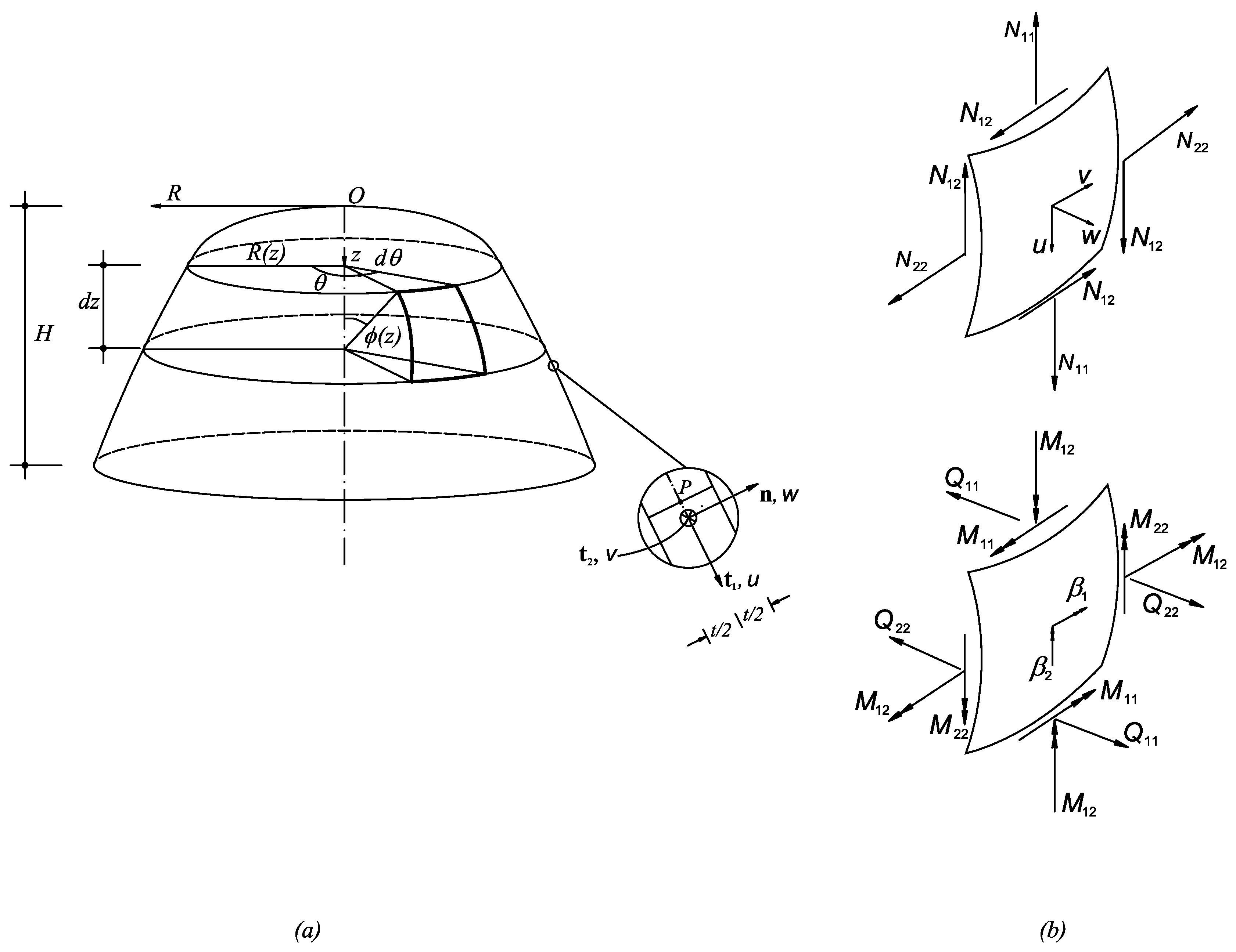
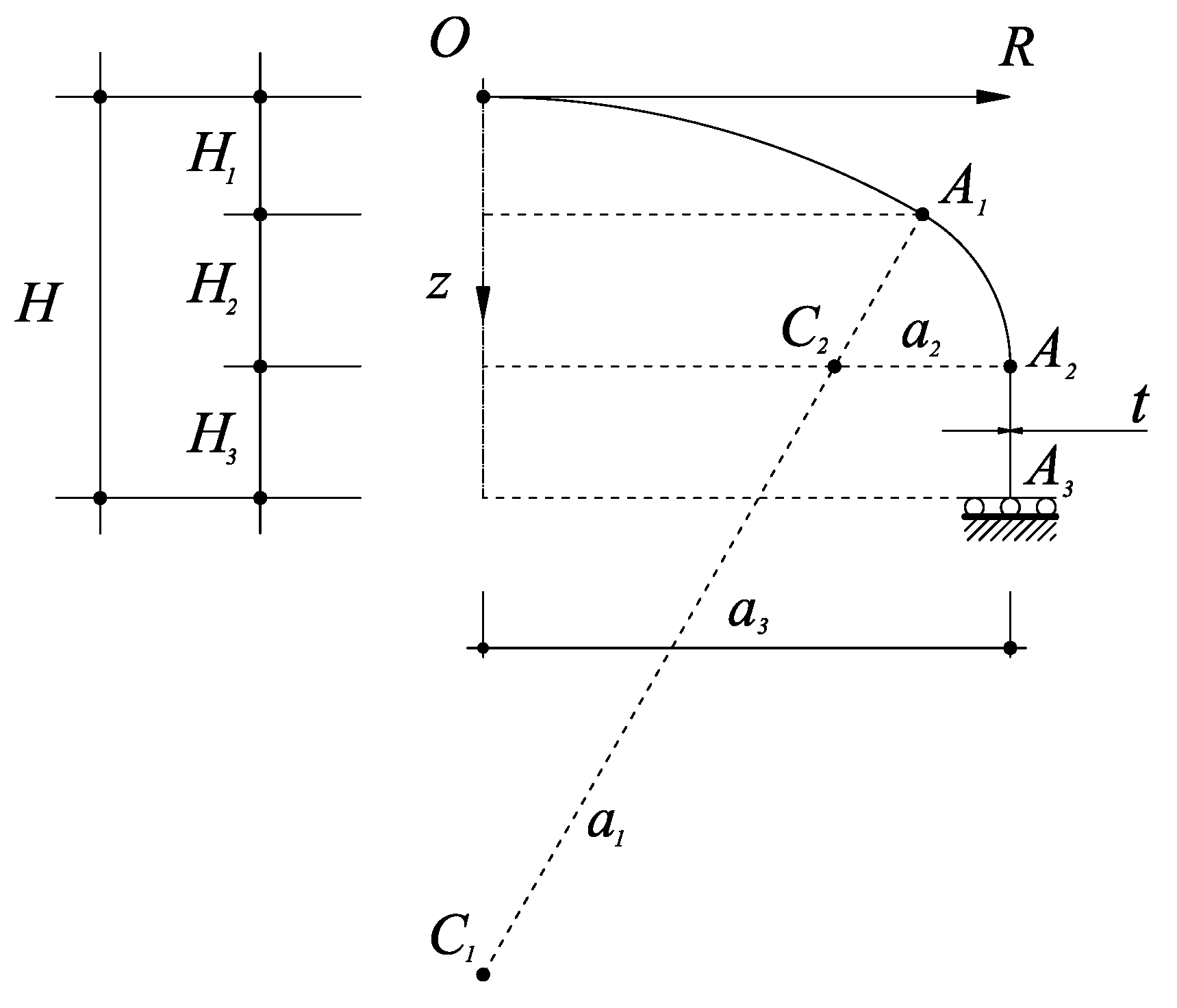
2.1. Geometry

We consider a shell of revolution defined by its mid-surface, obtained by rotating a plane generator curve around an axis to form a closed surface, as shown in Figure 1a. Curvilinear coordinates on the mid-surface are chosen to be associated to two families of mutually orthogonal curvilinear lines over the mid-surface, i.e., meridians and parallels, respectively. In particular, z is the coordinate measured along the axis of rotation, any value of z indicates a fixed parallel, whereas θ is the circumferential angle, indicating a given meridian. The third orthogonal coordinate is ζ, the distance of a point from the mid-surface, measured along $\mathbf{n}$, the outward unit normal to the mid-surface. The shell thickness will be denoted by t. Thus, the mid-surface can be described by the bounded open set:

$$\Omega =\{(z,\theta ,\zeta )\in {\mathbb{R}}^3|(z,\theta ,\zeta )\in (z_i,z_f)\times [0,2\pi ]\times \left\{0\right\}\}$$

(1)

and its boundary

$$\partial \Omega =\{(z,\theta ,\zeta )\in {\mathbb{R}}^3|(z,\theta ,\zeta )\in \{z_i,z_f\}\times [0,2\pi ]\times \left\{0\right\}\}$$

(2)

For subsequent developments, it is here assumed that description of shell geometry is given in terms of the parallel radius equation $R=R\left(z\right)$, which defines the shape of the meridian curve, plus the thickness variation $t=t\left(z\right)$, for $z\in [z_i,z_f]$. Nonetheless, it is pointed out that this hypothesis is not mandatory: $R\left(z\right)$ and $t\left(z\right)$ need not be specified analytically; i.e., they can be obtained from interpolated data, for instance with the use of NURBS basis functions [36]. According to the above geometry description, metrics of the shell of revolution mid-surface are resumed in Appendix A.

2.2. Displacement Field

Following the classical Reissner-Mindlin theory [37,38], and referring to Figure 1a, the displacements of a material point of the shell are u, v, and w, where u is the translation along ${\mathbf{t}}_1$, the unit vector tangent to the mid-surface and directed along the local meridian, v is the translation along ${\mathbf{t}}_2$, the unit vector tangent to the mid-surface and directed along the local parallel, and w is the displacement along $\mathbf{n}$, orthogonal to the mid-surface. Moreover, ${\beta }_1$ and ${\beta }_2$ represent the rotation of $\mathbf{n}$ about meridian ${\mathbf{t}}_1$ and circumferential ${\mathbf{t}}_2$ direction, respectively. In accordance with the aforementioned theory, the components u and v vary linearly with respect to ζ, while w, ${\beta }_1$, and ${\beta }_2$ are constant through the thickness. The degrees of freedom are collected in the algebraic vector:

$$\mathbf{u}(z,\theta )={\left[uvw{\beta }_1{\beta }_2\right]}^{\mathrm{T}}$$

(3)

depending on the mid-surface coordinates z and θ.

2.3. Internal Actions

In the present theory, equilibrium equations are written in terms of internal actions, or stress resultants and couples per curvilinear coordinate line unit length, defined as the integrals of the stress components through the shell thickness [37]. In Figure 1b, stress resultants and couples are represented acting on a mid-surface element, identified by two couples of curvilinear coordinate lines, having in-plane outward normal unit vectors ${\mathbf{t}}_1$ and ${\mathbf{t}}_2$, respectively. These internal actions can be grouped as membrane normal $N_{11}$, $N_{22}$, [resp. shearing $N_{12}$] forces; flexural bending $M_{11}$, $M_{22}$, [resp. twisting $M_{12}$] couples; and transverse shear forces $Q_{11}$, and $Q_{22}$, respectively. The set of stress resultants and couples are collected in the algebraic vector:

$$\mathbf{S}(z,\theta )={\left[N_{11}{N}_{22}{N}_{12}{M}_{11}{M}_{22}{M}_{12}{Q}_{11}{Q}_{22}\right]}^{\mathrm{T}}$$

(4)

Finally, $\mathbf{q}(z,\theta )={\left[q_u{q}_v{q}_{w}00\right]}^{\mathrm{T}}$ are surface distributed load components per unit mid-surface area corresponding to the degrees of freedom $\mathbf{u}$. Surface distributed bending loads are not considered in the present development.

2.4. Equilibrium

Following classical arguments [38], the free vibration problem, as well as the static equilibrium problem for a shell of revolution, are formulated as a set of five differential equations for the internal actions, a format which is classified as statically indetermined [37]. Nevertheless, the above problem may be formulated as five differential equations for displacements and rotations plus boundary conditions, introducing proper shell-like strain measures, defined through a strain-displacement linear differential operator and choosing an isotropic linear elastic constitutive law between internal actions and strain components (see Appendix A). The strain components are conjugate to internal actions $\mathbf{S}$, and are collected in the algebraic vector:

$$\mathit{\epsilon }(z,\theta )={\left[{\epsilon }_{11}{\epsilon }_{22}{\epsilon }_{12}{\kappa }_{11}{\kappa }_{22}{\kappa }_{12}{\chi }_1{\chi }_2\right]}^{\mathrm{T}}$$

(5)

where ${\epsilon }_{11}$, ${\epsilon }_{22}$ [resp. ${\epsilon }_{12}$] are membrane normal [resp. membrane shearing] strains, ${\kappa }_{11}$, ${\kappa }_{22}$ [resp. ${\kappa }_{12}$] are bending normal [resp. bending twisting] curvature variations, while ${\chi }_{11}$, and ${\chi }_{22}$ are transverse shearing strains. The equilibrium formulation amounts to a set of five linear differential equations for displacements and rotations $\mathbf{u}(z,\theta )$ on the two dimensional domain Ω, plus boundary conditions on $\partial \Omega$.

Applying Fourier series expansion of dependent variables (3), (4), and (5) with respect to the circumferential angle θ, the latter form can be reduced to a series of sets of five linear differential equations for the displacement harmonic amplitudes, on a one dimensional domain: the meridian curve. Since this treatment is quite consolidated [37,38,39,40], and the present work focuses on the Fourier series form of the equilibrium operator, for conciseness, we hereby present the displacement formulation in the so called harmonic form, postponing notations and the above recalled intermediate derivations to Appendix A and Appendix B.

2.4.1. Free Vibration Problem

The free vibration problem is governed by the classical linear eigenvalue problem:

$$\left\{\begin{array}{c}\text{Find}({\mathbf{u}}^{\left(j\right)},{\omega }^{\left(j\right)})\text{s.t.}\text{for}\text{any}\text{natural}\text{number}j,\hfill \\ {\mathcal{L}}^{\left(j\right)}\left({\mathbf{u}}^{\left(j\right)}\right)={\left({\omega }^{\left(j\right)}\right)}^2\mathcal{M}{\mathbf{u}}^{\left(j\right)},\forall z\in (z_i,z_f),\hfill \\ {\mathcal{B}}^{\left(j\right)}\left({\mathbf{u}}^{\left(j\right)}\right)=\mathbf{0},z\in \left\{z_i,z_f\right\}\hfill \end{array}\right.$$

(6)

where $({\mathbf{u}}^{\left(j\right)},{\omega }^{\left(j\right)})$ is the couple formed by the jth eigen-mode harmonic amplitude (in the sense specified in (35)), and the associated natural frequency. The inertia operator $\mathcal{M}$ is here taken as:

$$\mathcal{M}=\rho A_{1}R\mathrm{diag}\left\{ttt{t}^3/12t^3/12\right\}$$

where ρ is the material mass density [38].

2.4.2. Static Equilibrium Problem

The static equilibrium problem is governed by the following linear elliptic problem:

$$\left\{\begin{array}{c}\text{Find}{\mathbf{u}}^{\left(j\right)}\text{s.t.}\text{for}\text{any}\text{natural}\text{number}n,\hfill \\ {\mathcal{L}}^{\left(j\right)}\left({\mathbf{u}}^{\left(j\right)}\right)={\mathbf{q}}^{\left(j\right)},\forall z\in (z_i,z_f),\hfill \\ {\mathcal{B}}^{\left(j\right)}\left({\mathbf{u}}^{\left(j\right)}\right)=\mathbf{0},z\in \left\{z_i,z_f\right\}.\hfill \end{array}\right.$$

(7)

The equilibrium operator ${\mathcal{L}}^{\left(j\right)}$ and the boundary conditions operator ${\mathcal{B}}^{\left(j\right)}$ appearing in (6) and (7) are reported in Appendix A, depending on the equation $R=R\left(z\right)$, i.e., on the meridian shape, and on the relative metric quantities.

3. B-Spline Basis Functions

Non-Uniform Rational B-Splines - NURBS - are obtained from linear combination of B-Splines basis functions locally defined over patches of intervals [41]. A B-Spline of degree p is defined through an ordered set of non-decreasing coordinates in the parametric space: the knot vector $\Xi =\{{\xi }_1=0,{\xi }_2,\dots ,{\xi }_{n+p+1}=1\}$, where p represents the polynomial degree of the interpolation, and n is the number of basis functions associated to the knot vector. Consequently, it results that $p=0,1,2,3\dots$ refers to constant, linear, quadratic, cubic,... piecewise polynomials, respectively. An open knot vector has the first and the last knots repeated $p+1$ times ensuring that the basis functions are interpolatory at the extrema of the parametric space [41]. In the following, we assume uniform, i.e., equally spaced, open knot vectors.

The B-Spline basis functions $N_{i,p}$ can be defined starting with piecewise constants ($p=0$) by means of a recursive formula

$$N_{i,0}=\left\{\begin{array}{cc}1\hfill & \text{if}{\xi }_i\le \xi <{\xi }_{i+1}\hfill \\ 0\hfill & \text{otherwise}\hfill \end{array}i=1,2,...,n\right.$$

(8)

For $p=1,2,3,...$ it results:

$$N_{i,p}=\left\{\begin{array}{c}\frac{\xi -{\xi }_i}{{\xi }_{i+p}-{\xi }_i}{N}_{i,p-1}+\frac{{\xi }_{i+p+1}-\xi }{{\xi }_{i+p+1}-{\xi }_{i+1}}{N}_{i+1,p-1},\mathrm{if}{\xi }_i\le \xi <{\xi }_{i+p+1}\hfill \\ 0,\mathrm{otherwise}\hfill \end{array}\right.$$

Accordingly, basis functions of order p have $(p-1)$ continuous derivatives. If a knot is repeated k times, then the number of continuous derivatives decreases by k. A knot with multiplicity p, implies the basis functions to be interpolatory at that knot.

3.1. One Dimensional NURBS Interpolation

A non-uniform rational B-Spline in ${\mathbb{R}}^d$ is the projection onto d-dimensional physical space of a polynomial B-Spline defined in $(d+1)$-dimensional homogeneous coordinate space [41,42]. NURBS can be used to construct a vast gallery of geometrical entities, starting, for instance, from a discrete set of measured data [36]. The projective transformation of a B-Spline curve yields a rational polynomial curve. Inductively, the order p of a NURBS basis is identified as the order of the polynomial basis from which it was generated by projection.

A NURBS interpolation in ${\mathbb{R}}^d$ is constructed starting from a data set ${\mathbf{B}}_i^w$ $(i=1,...,n)$ or control points, for a B-Spline curve in ${\mathbb{R}}^{d+1}$ with knot vector Ξ. The control points for the NURBS curve are given by [41]:

$${\left(B_i\right)}_k=\frac{{\left(B_i^w\right)}_k}{w_i}k=1,...,d$$

(9)

where ${\left(B_i\right)}_k$ is the kth component of the vector $B_i$ and $w_i={\left(B_i^w\right)}_{d+1}$ is referred to as the ith weight. The NURBS basis functions of order p are then defined as:

$$R_{i,p}\left(\xi \right)=\frac{w_i{N}_{i,p}\left(\xi \right)}{{\sum }_{i=1}^n{w}_i{N}_{i,p}\left(\xi \right)}$$

(10)

Their first and second derivatives are given, respectively, by:

$${\left(R_{i,p}\right)}^{\prime }\left(\xi \right)=\frac{w_i{N}_{i,p}^{\prime }\left(\xi \right)}{{\sum }_{i=1}^n{w}_i{N}_{i,p}\left(\xi \right)w_i}-\frac{w_i{N}_{i,p}\left(\xi \right)N_{i,p}^{\prime }\left(\xi \right)w_i}{{\left({\sum }_{i=1}^n{w}_i{N}_{i,p}\left(\xi \right)\right)}^2}$$

(11)

and

$$\begin{array}{cc}{\left(R_{i,p}\right)}^{\prime \prime }\left(\xi \right)\hfill & =\frac{w_i{N}_{i,p}^{\prime \prime }\left(\xi \right)}{{\sum }_{i=1}^n{w}_i{N}_{i,p}\left(\xi \right)}+\hfill \\ & +\frac{2w_i{N}_{i,p}\left(\xi \right){\left({\sum }_{i=1}^n{w}_i{N}_{i,p}^{\prime }\left(\xi \right)\right)}^2}{{\left({\sum }_{i=1}^n{w}_i{N}_{i,p}\left(\xi \right)\right)}^3}+\hfill \\ & -\frac{2w_i{N}_{i,p}^{\prime }\left(\xi \right){\sum }_{i=1}^n{w}_i{N}_{i,p}^{\prime }\left(\xi \right)+w_i{N}_{i,p}\left(\xi \right){\sum }_{i=1}^n{w}_i{N}_{i,p}^{\prime \prime }\left(\xi \right)}{{\left({\sum }_{i=1}^n{w}_i{N}_{i,p}\left(\xi \right)\right)}^2}\hfill \end{array}$$

(13)

A pth degree NURBS curve is defined by:

$$\mathbf{C}\left(\xi \right)=\sum _{i=1}^n{R}_{i,p}\left(\xi \right)B_i$$

(13)

4. NURBS-Based Collocation Method

The main idea in the collocation method is to approximate the strong form of the equilibrium equations, without addressing a weak formulation typical of the finite element approach [8]. With reference to problem (6) or (7), the method consists in the approximation of the solution ${\mathbf{u}}^{\left(j\right)}$, $j=0,1,2,...$, as:

$${\tilde{\mathbf{u}}}^{\left(j\right)}=\sum _{i=1}^n{R}_{i,p}\left(\xi \right){\tilde{\mathbf{u}}}_i^{\left(j\right)}$$

(14)

where the interpolation functions $R_{i,p}\left(\xi \right)$ follow (10). The discrete form of (6)–(7) is thus obtained substituting (14) into the equilibrium operator ${\mathcal{L}}^{\left(j\right)}$ and into the boundary conditions operator ${\mathcal{B}}^{\left(j\right)}$, respectively. This leads to a set of $5n$ linear equations for the control values corresponding to (14). These unknown control values are obtained by enforcing the resulting discrete governing equations at n prescribed points in the parametric space, ${\xi }_c$ ($c=1,...,n$), defined collocation points:

• Free vibration problem

  $$\left\{\begin{array}{cc}{\mathcal{L}}^{\left(j\right)}\left({\tilde{\mathbf{u}}}^{\left(j\right)}\left({\xi }_c\right)\right)={\left({\omega }^{\left(j\right)}\right)}^2\mathcal{M}\left({\xi }_c\right)\left({\tilde{\mathbf{u}}}^{\left(j\right)}\left({\xi }_c\right)\right),\hfill & c=2,...,n-1\hfill \\ {\mathcal{B}}^{\left(j\right)}\left({\tilde{\mathbf{u}}}^{\left(j\right)}\left({\xi }_c\right)\right)=\mathbf{0},\hfill & c=1,n\hfill \end{array}\right.$$

  (15)
• Static equilibrium problem

  $$\left\{\begin{array}{cc}{\mathcal{L}}^{\left(j\right)}\left({\tilde{\mathbf{u}}}^{\left(j\right)}\left({\xi }_c\right)\right)=\mathbf{q}\left({\xi }_c\right),\hfill & c=2,...,n-1\hfill \\ {\mathcal{B}}^{\left(j\right)}\left({\tilde{\mathbf{u}}}^{\left(j\right)}\left({\xi }_c\right)\right)=\mathbf{0},\hfill & c=1,n\hfill \end{array}\right.$$

  (16)

Solution is thus obtained by solving for the unknown control values ${\tilde{\mathbf{u}}}_i^{\left(j\right)}$.

Collocation points are a set of natural coordinate values ${\xi }_c$, $c=1,...,n$, related to the knot vector. In the present case we will adopt the so called Greville nodes [36,43], i.e.,:

$${\xi }_c=\frac{1}{p}\sum _{k=c+1}^{c+p}{\xi }_k,c=1,...,n$$

(17)

The choice for collocation points is generally guided by an accuracy/efficiency criterion. The idea is to have a set of points for which known solutions of certain differential operators are exactly recovered by the numerical scheme [17,44,45,46]. The choice for collocating governing equations as in Equation (17) has proved efficient in previous NURBS-based collocation approaches [8,32,33], as it grants high-order accuracy and smoothness of the parametrization of the unknown with excellent convergence properties. Noteworthy, according to Johnson [46], Greville collocation points are associated to the property of linear precision [43], in the sense that if these are used to compute a B-Spline approximation of a straight line of the form $l\left(u\right)=au+b$, the corresponding B-Spline curve is a straight line.

Given the interesting performance of standard Lagrange interpolation spaces, for the implementation of 1D collocation methods for shells of revolution, reported by previous researches [13,14,15,16], in what follows, we explore the superior accuracy of the NURBS approximation in conjunction with the collocation approach. The attractiveness of this approximation is twofold: $\left(i\right)$ the NURBS high regularity suggests the possibility of obtaining smooth solutions even with low order approximation and low number of degrees of freedom, $\left(ii\right)$ the capability of describing complex geometries is interesting especially from a structural design point of view, when constructing geometrical models from measured data is required.

The discretization and solution of problem Equations (6) or (7) is programmed as follows:

• Define NURBS order p, number of control points n, build open knot vector Ξ, build NURBS basis and derivatives;
• Compute collocation points ${\xi }_c$, $c=1,2,...,n$;
• Parametrize curvilinear space coordinate $z=[z_i,z_f]$ as $z=z\left(\xi \right)$, and relevant geometric quantities, i.e., $R\left(z\right(\xi \left)\right)$, $A_1\left(z\left(\xi \right)\right)$, $sin\varphi \left(z\right(\xi \left)\right)$;
• Collocate above mentioned quantities at collocation points;
• Approximate equilibrium, mass matrix, and boundary conditions operators: ${\mathcal{L}}^{\left(j\right)}\left(z\left(\xi \right)\right)$, $\mathcal{M}\left(z\right(\xi \left)\right)$, and ${\mathcal{B}}^{\left(j\right)}\left(z\left(\xi \right)\right)$, respectively, and applied load distribution ${\mathbf{q}}^{\left(j\right)}\left(z\left(\xi \right)\right)$, through NURBS interpolants;
• Collocate discrete governing equations, i.e., equilibrium [resp. boundary condition] equations at internal [resp. boundary] collocation points;
• Assemble linear equations, viz. (15)–(16);
• Solve for ${\tilde{\mathbf{u}}}_i^{\left(j\right)}$, $j=0,1,...$;
• Post-process solution through NURBS interpolation.

As it is well known, such a discretization procedure does not lead to symmetric banded linear sets of equations as it is the case with finite element procedures. In particular, the coefficient matrix is sparse and nonsymmetric [44]; accordingly, factorization methods are generally not the most efficient, especially when dealing with large scale simulations. It is therefore recommended to resort to iterative methods such as conjugate gradient methods and residual based methods; is nonetheless noted that, albeit nonsymmetric, the pattern of coefficient matrices in displacement-based collocation approaches results competitive with respect to Galerkin finite element approaches which as known lead to symmetric systems [8].

5. Numerical Results

The present section is dedicated to numerical tests validating the NURBS collocation method for shells of revolution presented in the previous section. In subsection 5.1, we first present the asymptotic analysis of the fundamental eigenfrequency for shells of revolution of different Gaussian curvature (see (34)), an evidential benchmark test for assessing robustness with respect to membrane and shear locking in rotational shell numerical formulations. Secondly, we address the classical free vibration problem for different shells of revolution and different boundary conditions, comparing results with reference solutions. In subsection 5.2, a set of static problems are taken into consideration, in order to address the question of accuracy and convergence with respect to the order of interpolation and discretizaion. Finally, a simple technical problem is considered, validating the applicability of the present approach to problems of shell analysis and design, for shells with complex geometry.

5.1. Free Vibration Problems

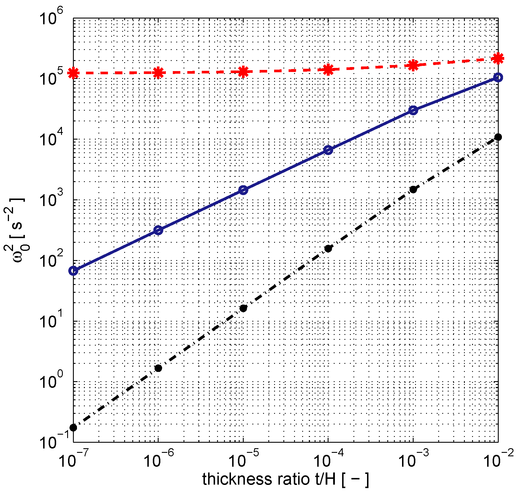
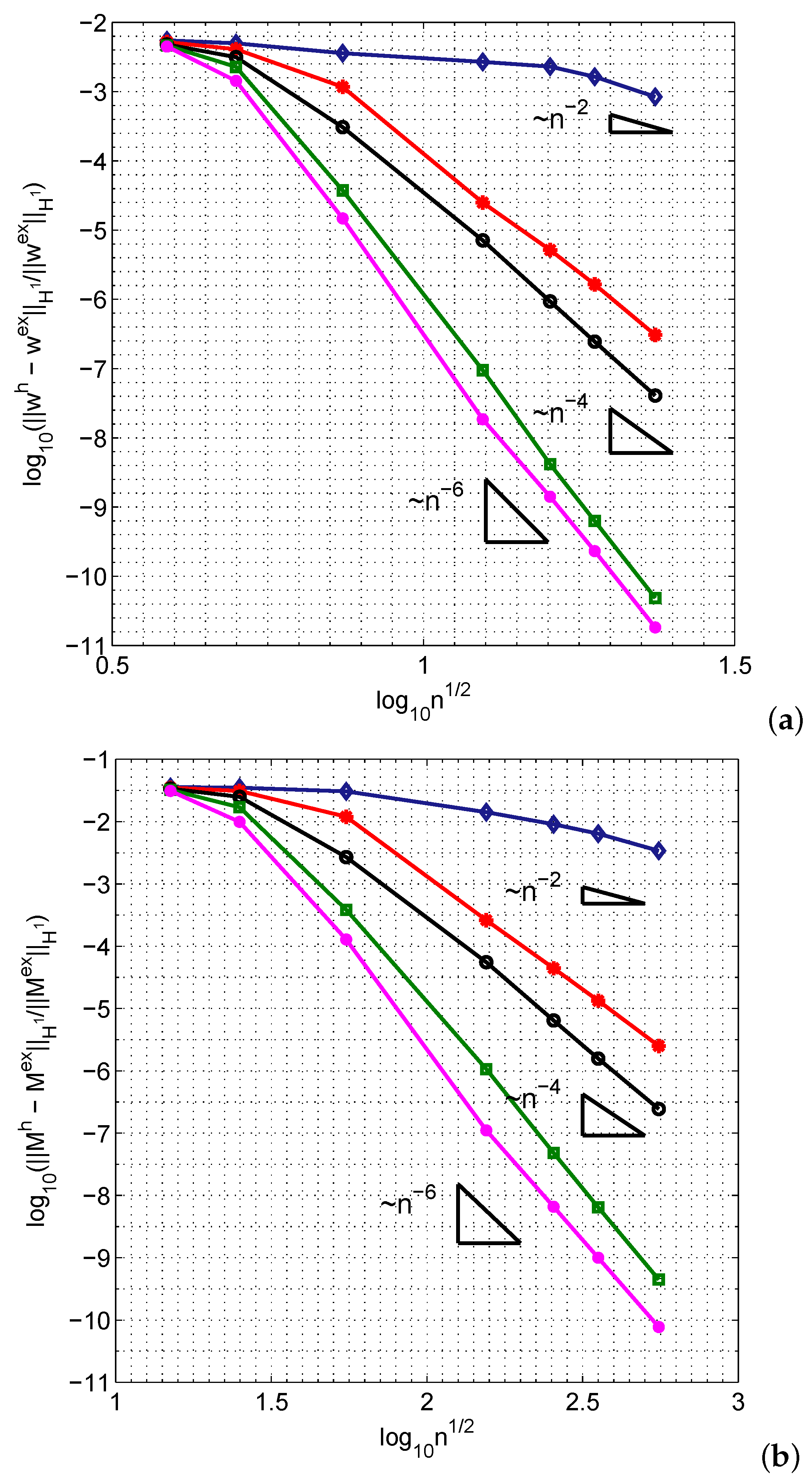
5.1.1. Asymptotic Analysis of Fundamental Frequency

Following [47,48,49], in this section we study the dependence of the lowest (fundamental) frequency on the thickness t as this quantity approaches zero. Three representative cases of Parabolic (zero Gaussian curvature), Elliptic (positive Gaussian curvature), and Hyperbolic (negative Gaussian curvature) shells of revolution are considered. The shells have clamped boundary conditions, in order to study the inhibited pure bending behavior [49]. The three cases reported in the following are characterized, respectively, by meridian equation of:

• Parabolic shape:

  $$R\left(z\right)=1,z\in [-H,H]$$

  (18)
• Elliptic shape:

  $$\begin{array}{cc}\hfill & R\left(z\right)=\sqrt[]{b^2\left(1-\frac{z^2}{a^2}\right)},z\in [-H,H]\hfill \end{array}$$

  (19)

  with $a^2=\frac{25}{9}{H}^2$, $b^2=H^2$;
• Hyperbolic shape:

  $$R\left(z\right)=\sqrt[]{a^2\left(1+\frac{z^2}{b^2}\right)},z\in [-H,H]$$

  (20)

  with $a^2=H^2$, $b^2=\frac{16}{9}{H}^2$.

and $H=1$. Material constants for the numerical simulations are $E=2.1\times {10}^{11}$ Pa, $\nu =0.3$, $\rho =7868$ $\mathrm{Kg}/{\mathrm{m}}^3$. The scope of this test is to check the asymptotic behaviors of the square of the fundamental, i.e., lowest, eigenfrequency ${\omega }_0^2$ when computed with the NURBS collocation method. In passing, it is recalled that the lowest eigenfrequency ${\omega }_0^2$ does not necessarily correspond to harmonic number $j=0$, nor any specific a-priori-known value j. Expected asymptotic rates are [47,50]:

• Parabolic shell:

  $$\underset{t\to 0}{lim}{\omega }_0^2=t$$

  (21)
• Elliptic shell:

  $$\underset{t\to 0}{lim}{\omega }_0^2=t^0$$

  (22)
• Hyperbolic shell:

  $$\underset{t\to 0}{lim}{\omega }_0^2=t^{2/3}$$

  (23)

In Figure 2 we report the logarithmic dependence of ${\omega }_t^2$ vs. thickness ratio $t/H$, for the three considered geometries. Accuracy in the low thickness range requires a fine discretization and high NURBS interpolation order, namely $n=101$ and $p=11$. In

Table 1. Asymptotic analysis of fundamental frequency ${\omega }_0^2$ with respect to thickness ratio $t/H$ for elliptic, parabolic, and hyperbolic shells of revolution. Slope values for different branch values in the asymptotic regime.

$t/H$	Parabolic	Slope	Elliptic	Slope	Hyperbolic	Slope
${10}^{-2}$	104.215276		464.007232		323.741324
		0.86531		0.11402		0.54346
${10}^{-3}$	38.483324		406.921457		173.166457
		0.97565		0.07091		0.65487
${10}^{-4}$	12.515376		375.017756		81.474984
		0.953114		0.03469		0.66104
${10}^{-5}$	4.025786		360.333432		38.062875
		0.98518		0.01484		0.66326
${10}^{-6}$	1.289914		354.228976		17.736469
		0.98857		0.00610		0.66686
${10}^{-7}$	0.417654		351.74876		8.211765

we report the eigenvalues at specified thickness values, delimiting subsequent thickness branches in the logarithmic scale. The slopes of these branches are in agreement with the theoretical prediction on asymptotic behavior of the fundamental frequency Equations (21)–(23). The above results prove the present method is capable of efficient treatment of situations in which geometry, boundary conditions and regularity of applied loads induce a so called intermediate state for which nor the bending strain energy or the membrane strain energy dominates on one another in the asymptotic regime, and interior or boundary layers concentrate the majority of the strain energy. Such situations are prone to numerical locking and strong instabilities in the solution [34,48]. In this regard, a necessary condition for a numerical scheme to be locking-free is given by Equations (21)–(23), which are satisfied by the present method.

5.1.2. Clamped Hemispherical Shell in Free Vibration

A clamped hemispherical dome with radius a and uniform thickness t ($a/t=100$), see Figure 3, is considered [51,52]. The values of the non-dimensional frequency parameter $\lambda =a{\omega }^{\left(j\right)}{(\rho /E)}^{1/2}$ are reported in

Table 2. Clamped hemispherical shell in free vibration. Non-dimensional frequency parameter $\lambda =a{\omega }^{\left(j\right)}{(\rho /E)}^{1/2}$. Reference results from [53] (parentheses) and from [14] (brackets).

Harmonic Number j	Mode Number m
	1	2	3	4	5	6
0	$0.761$	$0.939$	$0.988$	$1.029$	$1.087$	$1.172$
	$(0.761)$	$(0.938)$	$(0.984)$	$(1.021)$	$(1.021)$	$(-)$
	$[0.760]$	$[0.938]$	$[0.984]$	$[1.020]$	$[1.070]$	$[1.146]$
1	$0.567$	$0.893$	$0.965$	$1.003$	$1.047$	$1.112$
	$(0.567)$	$(0.894)$	$(0.966)$	$(1.002)$	$(1.046)$	$(1.106)$
	$[0.567]$	$[0.893]$	$[0.965]$	$[1.002]$	$[1.046]$	$[1.115]$
2	$0.901$	$0.966$	$0.998$	$1.030$	$1.079$	$1.151$
	$(0.901)$	$(0.966)$	$(0.998)$	$(1.031)$	$(1.081)$	$(1.153)$
	$[0.901]$	$[0.966]$	$[0.997]$	$[1.029]$	$[1.077]$	$[1.150]$
3	$0.947$	$0.989$	$1.023$	$1.065$	$1.121$	$1.203$
	$(0.948)$	$(0.990)$	$(1.024)$	$(1.066)$	$(1.124)$	$(1.207)$
	$[0.947]$	$[0.988]$	$[1.022]$	$[1.063]$	$[1.119]$	$[1.206]$
4	$0.969$	$1.005$	$1.043$	$1.094$	$1.162$	$1.259$
	$(0.969)$	$(1.005)$	$(1.045)$	$(1.095)$	$(1.167)$	$(1.264)$
	$[0.969]$	$[1.004]$	$[1.042]$	$[1.091]$	$[1.159]$	$[1.266]$
5	$0.984$	$1.020$	$1.065$	$1.124$	$1.208$	$1.321$
	$(0.985)$	$(1.021)$	$(1.066)$	$(1.127)$	$(1.213)$	$(1.327)$
	$[0.985]$	$[1.019]$	$[1.062]$	$[1.120]$	$[1.204]$	$[1.341]$

, for the first six modes and for different values of the harmonic number j. Reference results obtained with a Lagrange collocation method [14], and those from a Spline finite element solution by Luah and Fan [53] are reported for validation. The present frequency parameter values are obtained selecting $n=35$, $p=4$ for the lowest mode frequencies, up to $n=85$, $p=8$ for higher modes. Noteworthy, the closed apex condition required by this type of shell [16,37] can be modeled by the present approach straightforwardly, as it implies enforcement of special homogeneous Dirichlet boundary condition at $z=0$, depending on the harmonic number j:

$$\begin{array}{c}{u}^{\left(0\right)}=v^{\left(0\right)}={\beta }_1^{\left(0\right)}={\beta }_2^{\left(0\right)}=0\hfill \end{array}$$

(24)

$$\begin{array}{c}{u}^{\left(1\right)}+v^{\left(1\right)}=0,w^{\left(1\right)}=0,{\beta }_1^{\left(1\right)}+{\beta }_2^{\left(1\right)}=0\hfill \end{array}$$

(25)

$$\begin{array}{c}{u}^{\left(j\right)}=v^{\left(j\right)}=w^{\left(j\right)}={\beta }_1^{\left(j\right)}={\beta }_2^{\left(j\right)}=0,j\ge 2\hfill \end{array}$$

(26)

The present results are in agreement with the reference results, confirming the accuracy of the proposed technique, even for cases in which shear locking is expectable [54]. The method proves computationally efficient as even in the higher mode regime, the size of the eigenvalue problem is smaller than that associated to the reference results.

5.1.3. Simply supported circular plate in free vibration

A circular plate of radius a and thickness t, simply supported along the boundary, is considered. For conciseness, we shall refer to the shell geometry and boundary conditions as shown in Figure 7 even if related to the numerical test reported in Section 5.2.2. The non-dimensional parameter $\lambda ={[12(1-{\nu }^2)\rho a^4{\left({\omega }^{\left(j\right)}\right)}^2/\left(E{t}^2\right)]}^{1/2}$ computed with the present method is reported in Table 2, in agreement with reference values obtained in [14], and with those available from a Spline finite element approach by Luah and Fan [53]. The results confirm the interesting capabilities of the proposed approach for the free vibration analysis of rotational shells with different shapes and boundary conditions at a low computational cost. Numerical simulations show monotonic convergence to the computed eigenfrequencies, for increasing interpolation order p up to $p=5$, and discretization order n up to $n=35$. No spurious modes arise.

5.2. Static Equilibrium Problems

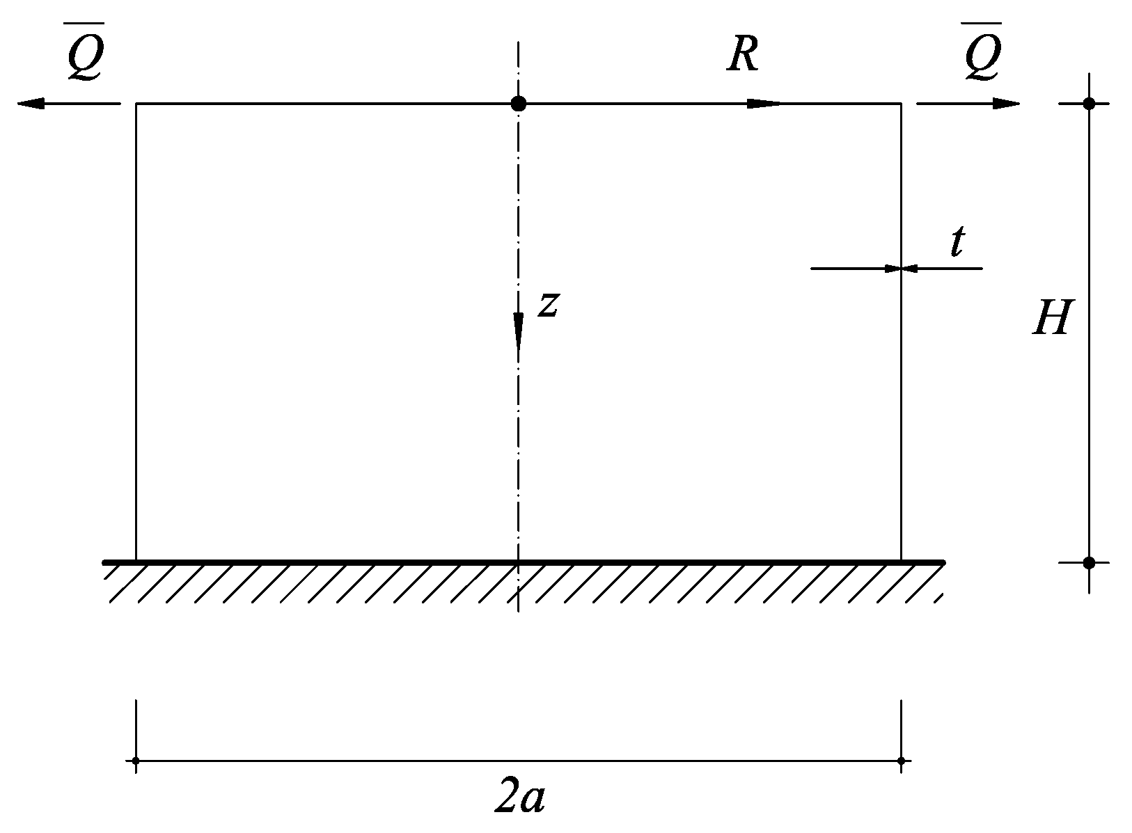
5.2.1. Cantilever Cylindrical Shell under Tip Load

A circular cylindrical shell, clamped at one end, with a uniform radial line load $\overline{Q}=1$ kN/m acting on the free edge, is considered, see Figure 4. The geometric data are $R=5$ m, $t=0.01$ m, $H=6$ m, the Young’s modulus and the Poisson ratio are, respectively, $E={10}^7$ kN/m${}^2$, and $\nu =0.3$. Axial symmetry permits to address the equilibrium problem for the $j=0$ harmonic only. The line load is taken into account by modifying the free boundary conditions at $z=0$, Equations (59)–(61), to guarantee that $Q_{11}$ equals the applied force on that boundary.

The present classical benchmark is here adopted as a tool for calibrating the model with respect to parameters n and p, i.e., mesh discretization ($h-$refinement) and order of interpolation ($p-$refinement), and for a given accuracy level. To this end, a reference solution proposed by Timoshenko and Woinowsky-Krieger [55] for semi-infinite circular cylindrical shells in axisymmetrical bending, is here taken into consideration for comparison and accuracy assessment. The structural behavior, which shifts from shear-flexural near the loaded edge to membrane dominated at the clamped boundary, is correctly reproduced by the NURBS-based collocation approach, as can be seen in Figure 5a,b, where $M_{11}$ and $Q_{11}$ are plotted, respectively, for an overkilling discretization with $n=250$ and $p=7$ with a relative error norm below ${10}^{-12}$, together with values computed through the reference solution at selected locations. The results are in agreement, plus the static boundary condition is exactly satisfied in solution.

Moreover, in order to assess the method convergence properties, we have plotted the $H^1$-error norms, of the tip transverse displacement $w\left(0\right)$, Figure 6a, and of bending moment $M_{11}\left(0\right)$, Figure 6b, for odd and even NURBS order p, and for increasing discretization refinements n. The asymptotic tendency of the error norm is consistent with analogous results reported in [31], where the static problem for Timoshenko spatial beams is addressed with a NURBS based collocation method. In particular, the logarithmic error is of the order $n^{-p}$ for any duplets of orders $(p,p+1)$, with even p, as theoretically predicted [32].

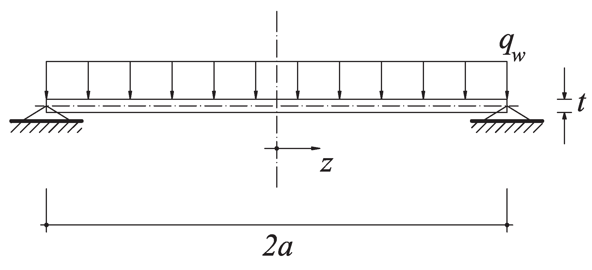
5.2.2. Simply Supported Circular Plate Subject to Uniform Pressure

We consider a simply supported circular plate under uniform normal load $q_w$, Figure 7. This benchmark has a closed-form solution, cfr. [56]. The material parameters are $E={10}^6$ kN/m${}^2$, $\nu =0.0$, the plate radius is $a=1$ m, the thickness is $t={10}^{-3}$ m, and the applied surface load is $q_w=1$ kN/m${}^2$. The load presents axial symmetry and requires to solve (7) for the $j=0$ harmonic only; closed apex conditions plus straight meridian geometry is fully taken into account by the present approach as the former amounts to special homogeneous Dirichlet boundary conditions (24), the latter is contemplated by (30)–(31). We report in

Table 4. Simply supported circular plate subject to uniform pressure. Comparison of present results for w, ${\beta }_1$, and $M_{11}$ at different locations z, for $cp=7$, $p=4$. Theoretical results from [56], reference results from [57].

	z [m]	Theor. [56]	Present	Ref. [57]
$w\times {10}^{-3}$ [m]	0.00	0.938	0.938	0.939
	0.25	0.868	0.868	0.868
	0.50	0.668	0.668	0.668
	0.75	0.364	0.364	0.364
	1.00	0	0	0
${\beta }_1\times {10}^{-3}$	0.00	0	0	0
	0.25	0.551	0.551	0.551
	0.50	1.031	1.031	1.031
	0.75	1.371	1.371	1.371
	1.00	1.500	1.500	1.500
$M_{11}$ [kN m/m]	0.00	0.188	0.188	0.188
	0.25	0.176	0.176	0.176
	0.50	0.141	0.141	0.141
	0.75	0.082	0.082	0.082
	1.00	0	0	$3\times {10}^{-14}$

the results obtained with the present approach, compared with an analytical solution [37], and with a hybrid mixed rotational finite element solution [57]. A space discretization characterized by $n=7$ and $p=4$ is sufficient to obtain accurate results. Resorting to the NURBS basis structure, post-processed quantities such as the bending and twisting moments in Figure 8a, and the rotation degrees of freedom in Figure 8b, can be plotted.

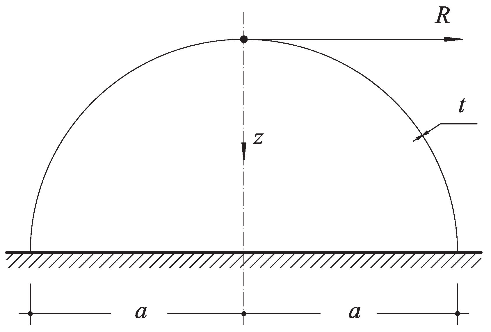
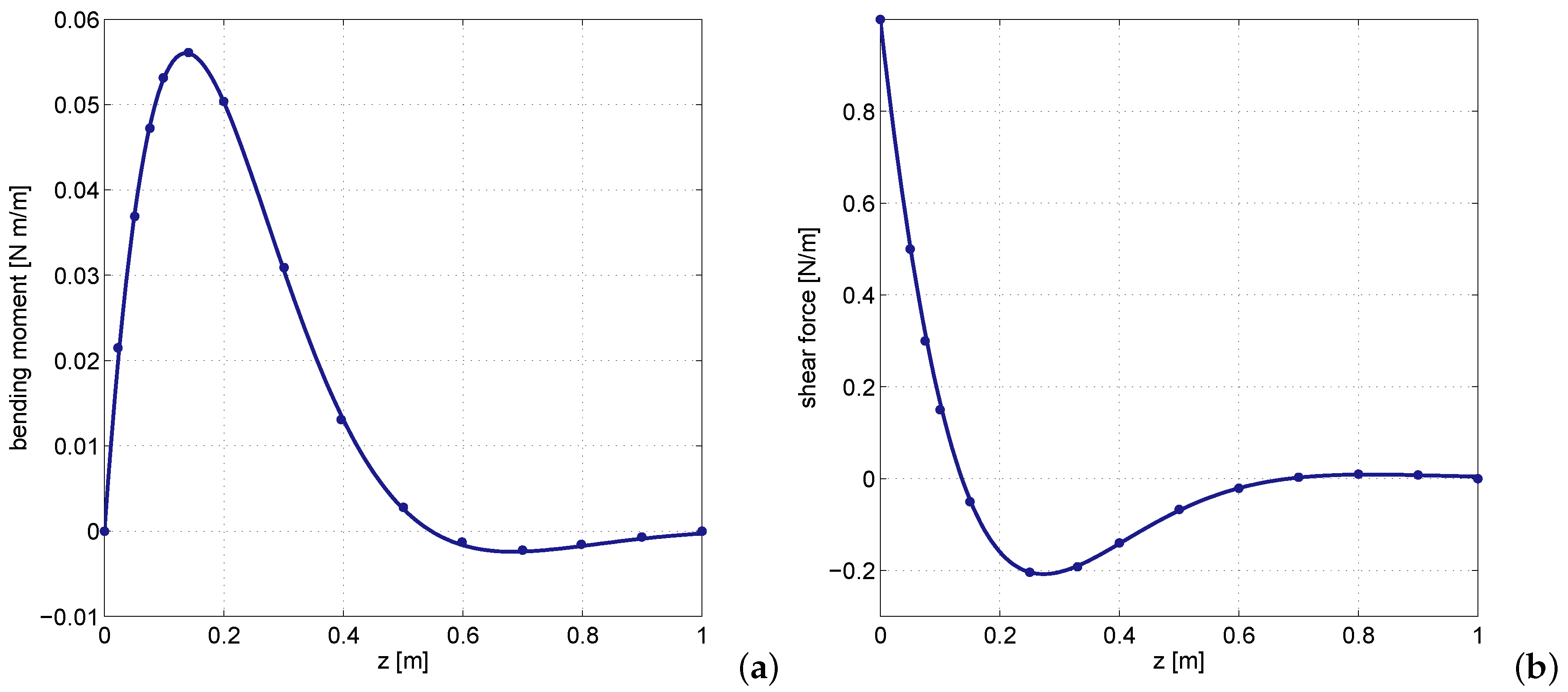
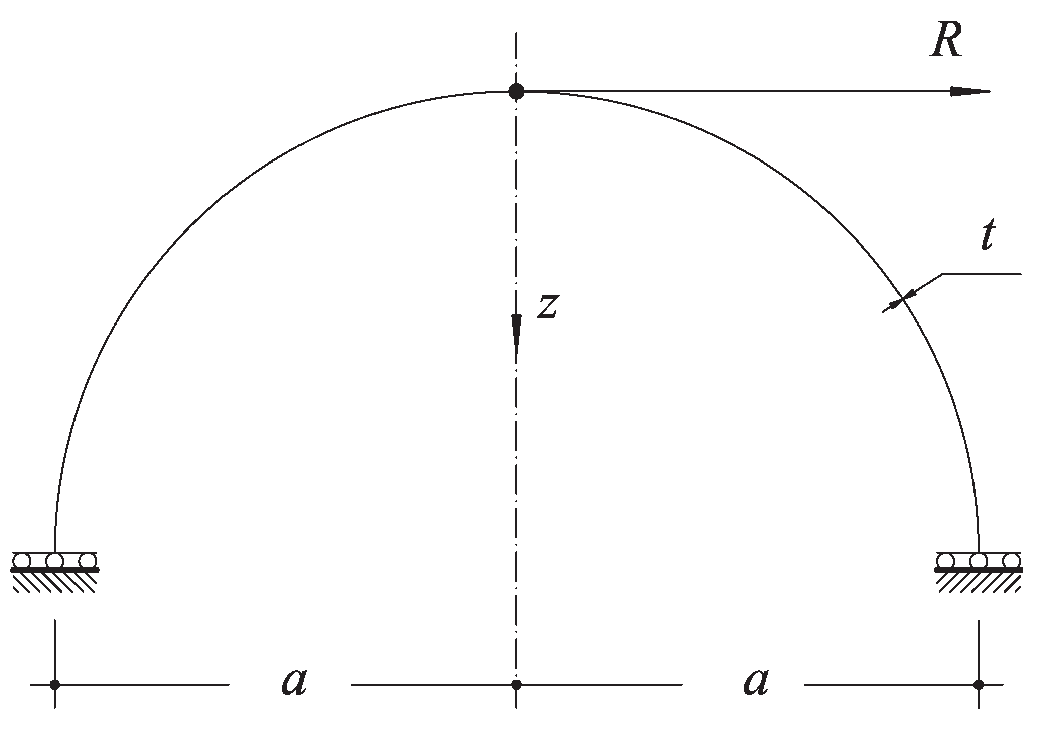
5.2.3. Hemispherical Shell under Uniform Pressure

This numerical test presents a spherical shell of radius $a=1$ and uniform thickness $t=0.01$, see Figure 9. The shell is loaded by a uniform internal pressure $q_w=1$. The Young modulus is $E=2.1\times {10}^{11}$ and the Poisson ratio is $\nu =0.3$. Due to symmetry, only the upper half shell is modeled, with closed apex conditions at $z=0$ and sliding edge boundary condition at $z=R$. The solution for displacement and strain components is expected to in a pure membrane dominated regime with zero shear/bending deformation. Henceforth, given the aim of the present test, no reference solution is here taken into account. The NURBS collocation is applied with $n=35$ and $p=5$, sufficient to grant the exact solution reported in the following. The results shown in Figure 10a,b for displacement and strain components are in agreement with theory, in particular zero tangential displacements v as well as null membrane shearing strains ${\epsilon }_{12}$ are correctly recovered, for a pure membrane equilibrium state of the spherical shell characterized by ${\epsilon }_{11}={\epsilon }_{22}$. It is readily checked that curvature variations and shear strains are identically zero as expected.

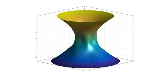
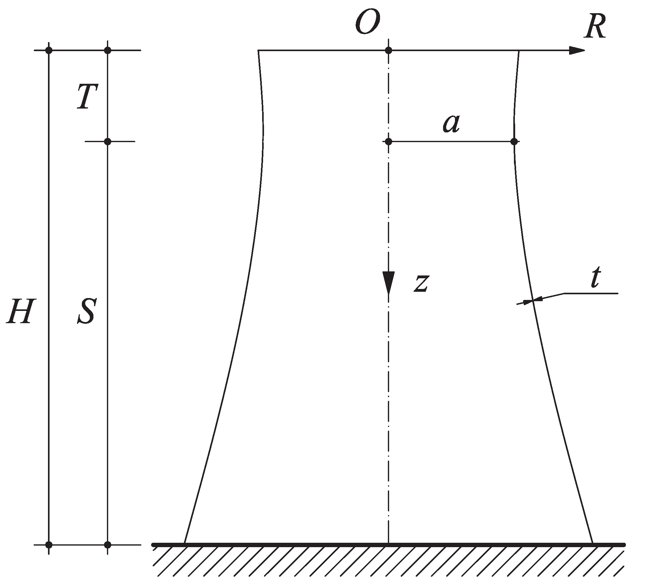
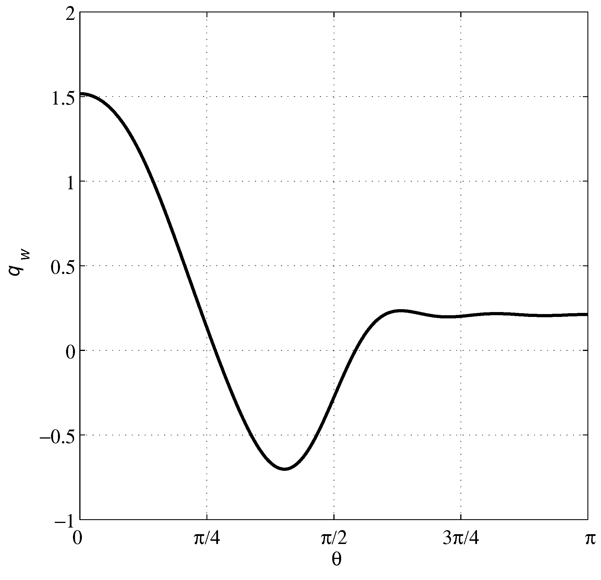
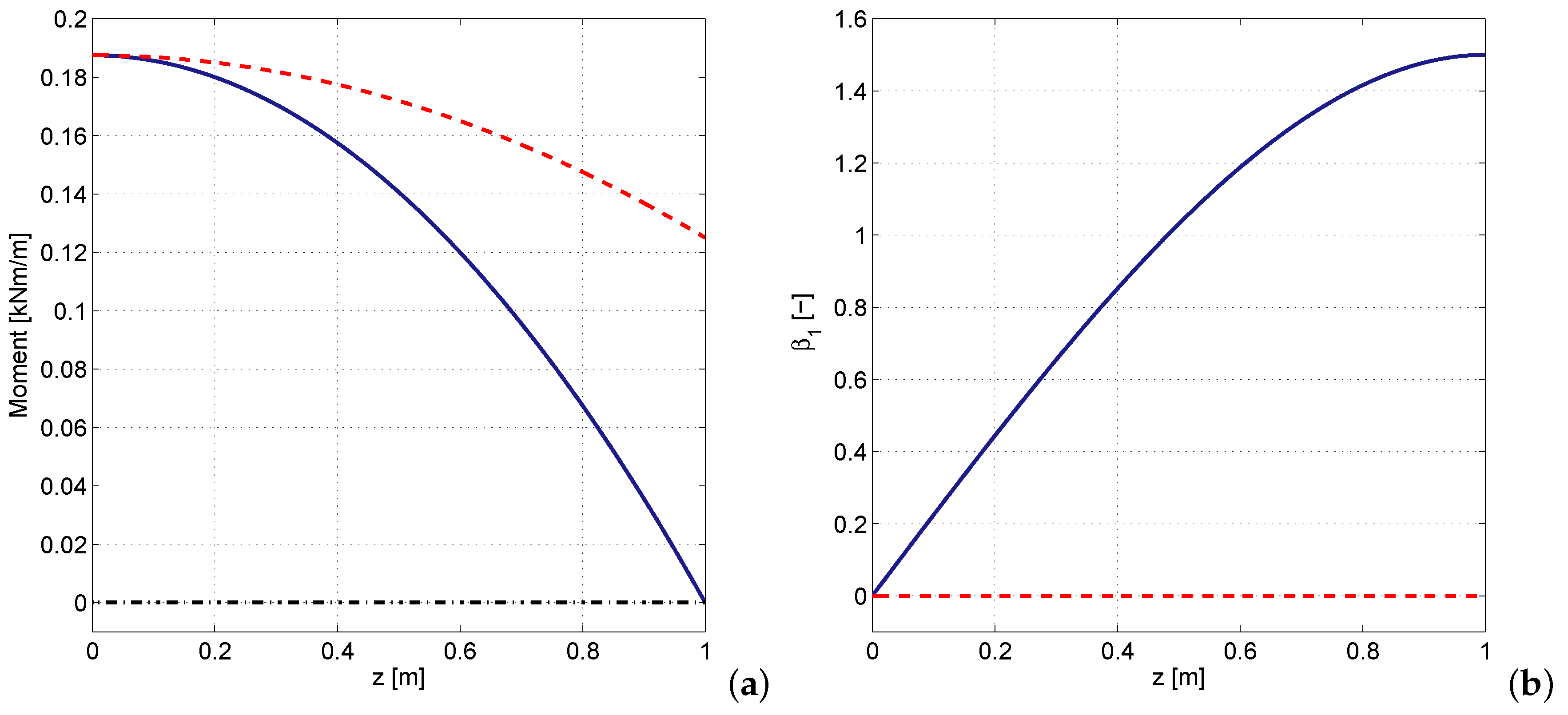
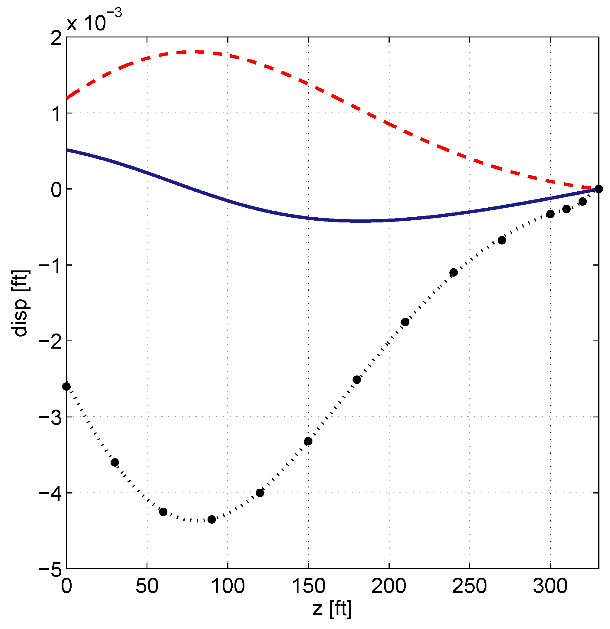
5.2.4. Hyperboloid of Revolution under Wind Load

The example presents a doubly curved hyperboloid of revolution, a typical cooling tower structure, Figure 11, subject to wind pressure. Geometrical data for the shell are, $a=84$ ft, $T=60$ ft, $H=330$ ft, $t=7$ in. The Young modulus is $E=432\times {10}^6\mathrm{lb}/{\mathrm{ft}}^2$, Poisson ratio is $\nu =0.15$. The surface load $q_w$ is constant along the tower height, and is not symmetric with respect to the axis of revolution; in particular, $q_w$ varies with the circumferential coordinate θ as reported in Figure 12 [57]. The distributed load is expanded in Fourier series taking into account the first ten harmonic components $j=0,1,...,9$. The present analysis aims at determining both displacements and stress resultants for the structure, which are respectively plotted in Figure 13 and Figure 14, where a comparison with different reference solutions available in the literature is carried out [58], together with a reference solution computed with SHORE III, a ring finite element code developed by [59]. The proposed methodology yields reliable results for $n=35$ and $p=8$ even for the case of a doubly curved rotational shell with unsymmetrical loading, which produces complex stress resultants and couples patterns. The numerical test confirms the present method capability of analyzing real shell structures under complex loading conditions with favorable accuracy.

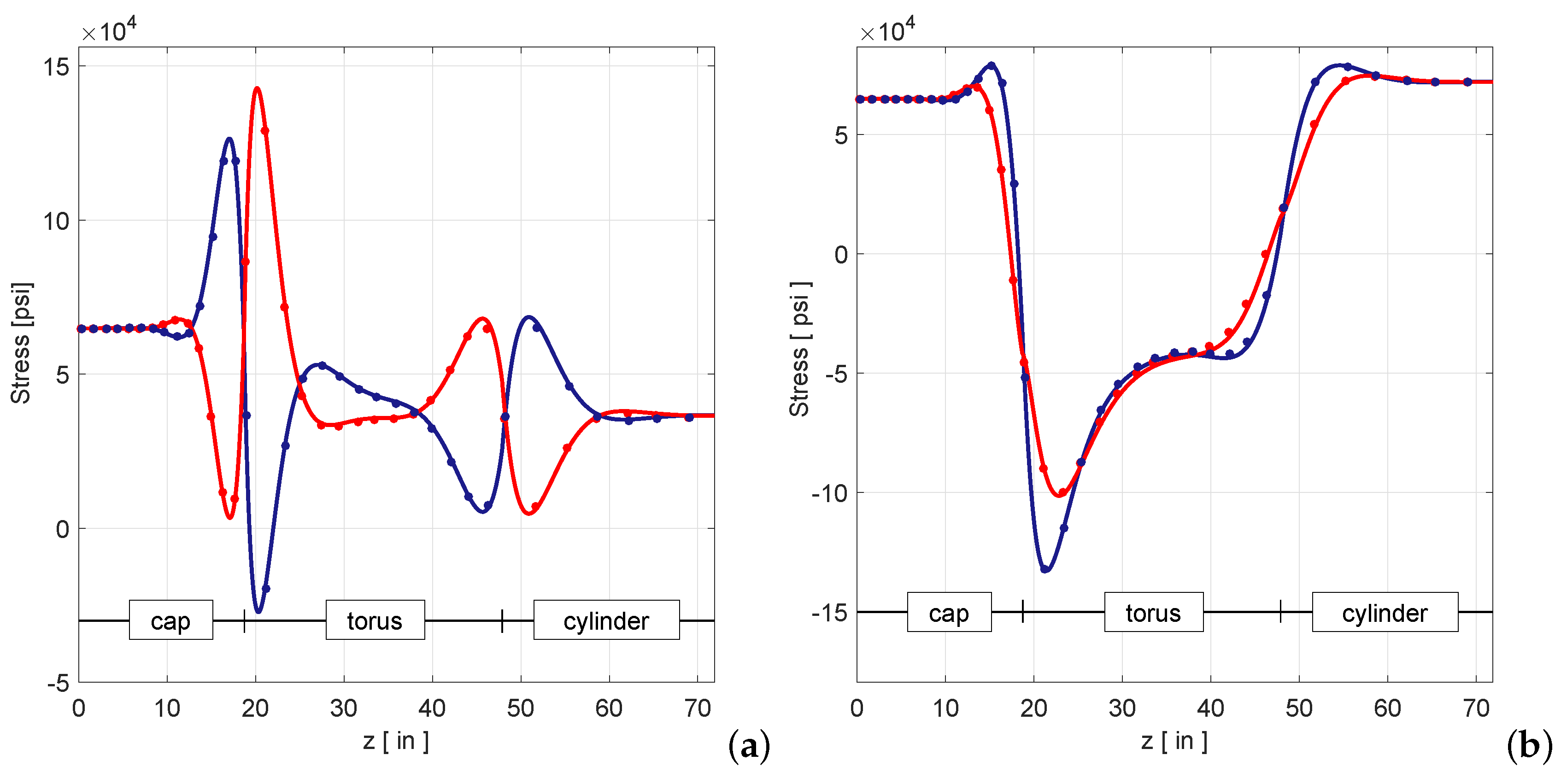
5.2.5. Torispherical tank subject to uniform internal pressure

The example presents a technical problem for a so called compound shell, namely a shell of revolution obtained by the smooth blending of different shell segments, each having a particular meridian curve geometry [37], see Figure 15. The shell comprises a closed-apex spherical cap $O{A}_1$ of radius $a_1=172.8981$ in. and length $H_1=18.675$ in., a torus segment $A_1{A}_2$ of radius $a_2=32.74$ in. and length $H_2=29.2$ in., and a cylindrical portion with radius $a_3=96.1$ in. and length $H_3=24$ in.; the thickness t is uniformly equal to $0.20$ in. The Young modulus is $E=3.0\times {10}^4$ psi, the Poisson ratio is $\nu =0.3$.

In order to model the pre-buckling elastic stress pattern, which is known to induce particularly severe compressive circumferential stresses in the toroidal region, the shell is loaded by a uniform internal pressure $q_w=150$ psi [37]. The geometry in the present analysis is constructed using three different NURBS control polygons, each one pertaining to a single shell segment, and each set with an equal number of basis functions. The three subdomains are then patched together, granting regularity of the meridian at the junctions and $C^0$ continuity of displacements and rotations, a procedure referred to as domain decomposition [44,45]. Nonetheless, it is pointed out that it is possible to use a single basis to describe the entire geometry and to collocate governing equations over the single control polygon. NURBS basis for collocation is characterized by $n=55$ on the spherical and toroidal segments, and $n=7$ on the cylindrical region. The order of the interpolants is $p=5$. The reference solution for this benchmark is provided by the finite element code SHORE III, adopting a fine mesh discretization with 128 quartic displacement based elements on both spherical and toroidal parts, and with 8 elements on the cylindrical segment. Results and comparison are plotted in Figure 16, reporting displacements u and w, and in Figure 17 for rotation ${\beta }_1$. Figure 18a [resp. Figure 18b] show the axial ${\sigma }_{11}$ and circumferential ${\sigma }_{22}$ normal stress components at inner ($\zeta =-t/2$) and outer ($\zeta =t/2$) surface of the shell [60]:

$${\sigma }_{ii}=\frac{N_{ii}}{t}\pm \frac{6M_{ii}}{t^2}i=1,2$$

(27)

obtained by post processing of stress resultants and couples. Remarkably good agreement is observed between present and reference results, confirming the capability of the proposed technique to study complex technically relevant problems for shells of revolution, as the aforementioned pre-buckling analysis of a cylindrical tank with torispherical head.

6. Conclusions

In this paper we have presented a NURBS-based collocation method for the elastic analysis of shells of revolution. Both the free vibration and the static equilibrium problems have been investigated in the realm of Reissner-Mindlin theory. Use of Fourier series expansion of dependent variables with respect to the circumferential angle permits to solve the problem as a series of one-dimensional differential equation sets. A NURBS-based collocation method has been presented exploiting the superior behavior of such interpolation methodology which grants higher order accuracy and regularity. The proposed method has been tested on different free vibration and static equilibrium benchmark problems, showing its versatility and accuracy in computing free vibration modes and frequencies, as well as stresses and displacement patterns. Comparison with existing results seems encouraging and confirm the interesting approximation properties of NURBS basis functions which grant avoidance of numerical problems such as locking and instability. The robustness shown by the proposed methodology suggests implementation into a general purpose code for the structural analysis and design of complex shell structures.

References

1. Bellman, R. Differential quadrature and long-term integration. J. Math. Anal. Appl. 1971, 34, 235–238. [Google Scholar] [CrossRef]
2. Bellman, R.; Kashef, B.G.; Casti, J. Differential quadrature: A technique for the rapid solution of nonlinear partial differential equations. J. Comput. Phys. 1972, 10, 40–52. [Google Scholar] [CrossRef]
3. Petersen, I. Convergence of approximate methods of the interpolation type for ordinary differential equations. Izv. Akad. Nauk. SSR 1961, 1, 3–12. [Google Scholar]
4. Karpilovskaya, E.B. Convergence of the collocation method. Proc. USSR Acad. Sci. 1963, 151, 766–769. [Google Scholar]
5. Vainikko, G. Convergence and stability of the collocation method. Differ. ur-niya 1965, 1, 244–254. [Google Scholar]
6. Vainikko, G. The convergence of the collocation method for non-linear differential equations. USSR Comput. Math. Math. Phys. 1966, 6, 47–58. [Google Scholar] [CrossRef]
7. Kaspshitskaya, M.F.; Luchka, A.Y. The collocation method. USSR Comput. Math. Math. Phys. 1968, 8, 19–39. [Google Scholar] [CrossRef]
8. Schillinger, D.; Evans, J.A.; Reali, A.; Schott, M.; Hughes, T.J.R. Isogeometric collocation: Cost comparison with galerkin methods and extension to adaptive hierarchical nurbs discretizations. Comput. Methods Appl. Mech. Eng. 2013, 267, 170–232. [Google Scholar] [CrossRef]
9. Bert, C.W.; Malik, M. Differential quadrature: A powerful new technique for analysis of composite structures. Compos. Struct. 1997, 39, 179–189. [Google Scholar] [CrossRef]
10. Mirfakhraei, P.; Redekop, D. Buckling of circular cylindrical shells by the differential quadrature method. Int. J. Press. Vessel. Pip. 1998, 75, 347–353. [Google Scholar] [CrossRef]
11. Wu, T.; Liu, G. Axisymmetric bending solution of shells of revolution by the generalized differential quadrature rule. Int. J. Press. Vessel. Pip. 2000, 77, 149–157. [Google Scholar] [CrossRef]
12. Wu, T.; Wang, Y.; Liu, G. A generalized differential quadrature rule for bending analysis of cylindrical barrel shells. Comput. Methods Appl. Mech. Eng. 2003, 192, 1629–1647. [Google Scholar] [CrossRef]
13. Artioli, E.; Viola, E. Static analysis of shear-deformable shells of revolution via G.D.Q. method. Struct. Eng. Mech. 2005, 19, 459–475. [Google Scholar] [CrossRef]
14. Viola, E.; Artioli, E. The G.D.Q. method for the harmonic dynamic analysis of rotational shell structural elements. Struct. Eng. Mech. 2004, 17, 789–817. [Google Scholar] [CrossRef]
15. Artioli, E.; Gould, P.L.; Viola, E. A differential quadrature method solution for shear-deformable shells of revolution. Eng. Struct. 2005, 27, 1879–1892. [Google Scholar] [CrossRef]
16. Artioli, E.; Viola, E. Free vibration analysis of spherical caps using a G.D.Q. numerical solution. ASME J. Press. Vessel. Technol. 2006, 128, 370–378. [Google Scholar] [CrossRef]
17. Bellman, R.; Kashef, B.; Lee, E.; Vasudevan, R. Differential quadrature and splines. Comput. Math. Appl. 1975, 1, 371–376. [Google Scholar] [CrossRef]
18. Guo, Q.; Zhong, H. Non-linear vibration analysis of beams by a spline-based differential quadrature method. J. Sound Vib. 2004, 269, 413–420. [Google Scholar] [CrossRef]
19. Zhong, H. Spline-based differential quadrature for fourth order differential equations and its application to kirchhoff plates. Appl. Math. Model. 2004, 28, 353–366. [Google Scholar] [CrossRef]
20. Huang, D. Analysis of laminated plates and shells by using spline gauss collocation method. Comput. Struct. 1991, 38, 469–473. [Google Scholar] [CrossRef]
21. Viswanathan, K.; Lee, S.K. Free vibration of laminated cross-ply plates including shear deformation by spline method. Int. J. Mech. Sci. 2007, 49, 352–363. [Google Scholar] [CrossRef]
22. Viswanathan, K.; Navaneethakrishnan, P. Free vibration study of layered cylindrical shells by collocation with splines. J. Sound Vib. 2003, 260, 807–827. [Google Scholar] [CrossRef]
23. Viswanathan, K.; Navaneethakrishnan, P. Free vibration of layered truncated conical shell frusta of differently varying thickness by the method of collocation with cubic and quintic splines. Int. J. Solids Struct. 2005, 42, 1129–1150. [Google Scholar] [CrossRef]
24. Bazilevs, Y.; Calo, V.M.; Cottrell, J.A.; Evans, J.A.; Hughes, T.J.R.; Lipton, S.; Scott, M.A.; Sederberg, T.W. Isogeometric analysis using t-splines. Comput. Methods Appl. Mech. Eng. 2010, 199, 229–263. [Google Scholar] [CrossRef]
25. Cottrell, J.A.; Hughes, T.J.R.; Reali, A. Studies of refinement and continuity in isogeometric structural analysis. Comput. Methods Appl. Mech. Eng. 2007, 196, 4160–4183. [Google Scholar] [CrossRef]
26. Cottrell, J.A.; Reali, A.; Bazilevs, Y.; Hughes, T.J.R. Isogeometric analysis of structural vibrations. Comput. Methods Appl. Mech. Eng. 2006, 195, 5257–5296. [Google Scholar] [CrossRef]
27. Hughes, T.J.R.; Cottrell, J.A.; Bazilevs, Y. Isogeometric analysis: Cad, finite elements, nurbs, exact geometry and mesh refinement. Comput. Methods Appl. Mech. Eng. 2005, 194, 4135–4195. [Google Scholar] [CrossRef]
28. Hughes, T.J.R.; Reali, A.; Sangalli, G. Duality and unified analysis of discrete approximations in structural dynamics and wave propagation: Comparison of p-method finite elements with k-method nurbs. Comput. Methods Appl. Mech. Eng. 2008, 197, 4104–4124. [Google Scholar] [CrossRef]
29. Hughes, T.J.R.; Reali, A.; Sangalli, G. Efficient quadrature for nurbs-based isogeometric analysis. Comput. Methods Appl. Mech. Eng. 2010, 199, 301–313. [Google Scholar] [CrossRef]
30. Auricchio, F.; da Veiga, L.B.; Hughes, T.J.R.; Reali, A.; Sangalli, G. Isogeometric collocation methods. Math. Models Methods Appl. Sci. 2010, 20, 2075–2107. [Google Scholar] [CrossRef]
31. Auricchio, F.; da Veiga, L.B.; Hughes, T.J.R.; Reali, A.; Sangalli, G. Isogeometric collocation for elastostatics and explicit dynamics. Comput. Methods Appl. Mech. Eng. 2012, 249–252, 2–14. [Google Scholar] [CrossRef]
32. Auricchio, F.; da Veiga, L.B.; Kiendl, J.; Lovadina, C.; Reali, A. Locking-free isogeometric collocation methods for spatial timoshenko rods. Comput. Methods Appl. Mech. Eng. 2013, 263, 113–126. [Google Scholar] [CrossRef]
33. Da Veiga, L.B.; Lovadina, C.; Reali, A. Avoiding shear locking for the timoshenko beam problem via isogeometric collocation methods. Comput. Methods Appl. Mech. Eng. 2012, 241–244, 38–51. [Google Scholar] [CrossRef]
34. Da Veiga, L.B.; Lovadina, C. An interpolation theory approach to shell eigenvalue problems. Math. Models Methods Appl. Sci. 2008, 18, 2003–2018. [Google Scholar] [CrossRef]
35. Finlayson, B.; Scriven, L. The method of weighted residuals—A review. Appl. Mech. Rev. 1966, 19, 735–748. [Google Scholar]
36. Farin, G. Curves and Surfaces for Computer Aided Geometric Design; Morgan Kaufman Publishers: San Francisco, CA, USA, 2002. [Google Scholar]
37. Gould, P.L. Finite Element Analysis of Shells of Revolution; Pitman Advanced Publishing Program: New York, NY, USA, 1985. [Google Scholar]
38. Kraus, H. Thin Elastic Shells; John Wiley & Sons: New York, NY, USA, 1967. [Google Scholar]
39. Novozhilov, V.V. Thin Shell Theory; Wolters-Noordhoff: Groningen, The Netherlands, 1970. [Google Scholar]
40. Soedel, W. Vibrations of Shells and Plates; Marcel Dekker, Inc.: New York, NY, USA, 2004. [Google Scholar]
41. Piegl, L.; Tiller, W. The NURBS Book, 2nd ed.; Springer-Verlag: Berlin Heidelberg Germany, 1997. [Google Scholar]
42. Rogers, D. An Introduction to NURBS with Historical Perspective; Morgan Kaufman Publishers: San Francisco, CA, USA, 2001. [Google Scholar]
43. Greville, T. On the normalization of the b-splines and the location of the nodes for the case of unequally spaced knots. In Inequalities; Oshida, O., Ed.; Academic Press: New York, NY, USA, 1967. [Google Scholar]
44. Bellomo, N. Nonlinear models and problems in applied sciences from differential quadrature to generalized collocation methods. Math. Comput. Model. 1997, 26, 13–34. [Google Scholar] [CrossRef]
45. Bellomo, N.; De Angelis, E.; Graziano, L.; Romano, A. Solution of nonlinear problems in applied sciences by generalized collocation methods and mathematica. Comput. Math. Appl. 2001, 41, 1343–1363. [Google Scholar] [CrossRef]
46. Johnson, R.W. Higher order b-spline collocation at the greville abscissae. Appl. Numer. Math. 2005, 52, 63–75. [Google Scholar] [CrossRef]
47. Artioli, E.; da Veiga, L.B.; Hakula, H.; Lovadina, C. Free vibrations for some koiter shells of revolution. Appl. Math. Lett. 2008, 21, 1245–1248. [Google Scholar] [CrossRef]
48. Auricchio, F.; da Veiga, L.B.; Lovadina, C. Remarks on the asymptotic behaviour of Koiter shells. Comput. Struct. 2002, 80, 735–745. [Google Scholar] [CrossRef]
49. Da Veiga, L.B.; Lovadina, C. Asymptotics of shell eigenvalue problems. C. R. Math. 2006, 342, 707–710. [Google Scholar] [CrossRef]
50. Artioli, E.; da Veiga, L.B.; Hakula, H.; Lovadina, C. On the asymptotic behaviour of shells of revolution in free vibration. Comput. Mech. 2009, 44, 45–60. [Google Scholar] [CrossRef]
51. Altman, W.; Neto, E.L. Vibration of thin shells of revolution based on a mixed finite element formulation. Comput. Struct. 1986, 23, 291–303. [Google Scholar] [CrossRef]
52. Kunieda, H. Flexural axisymmetric free vibrations of a spherical dome: exact results and approximate solutions. J. Sound Vib. 1984, 92, 1–10. [Google Scholar] [CrossRef]
53. Luah, M.H.; Fan, S.C. General free vibration analysis of shells of revolution using the spline finite element method. Comput. Struct. 1989, 33, 1153–1162. [Google Scholar] [CrossRef]
54. Kim, J.G.; Kim, Y.Y. Higher-order hybrid-mixed axisymmetric thick shell element for vibration analysis. Int. J. Numer. Meth. Eng. 2001, 51, 241–252. [Google Scholar] [CrossRef]
55. Timoshenko, S.; Woinowsky-Krieger, S. Theory of Plates and Shells; Mcgraw-Hill: New York, NY, USA, 1959. [Google Scholar]
56. Reddy, J.N. Energy and Variational Methods in Applied Mechanics; John Wiley & Sons: New York, NY, USA, 1984. [Google Scholar]
57. Kim, J.G.; Kim, Y.Y. A higher-order hybrid-mixed harmonic shell-of-revolution element. Comp. Meth. Appl. Mech. Eng. 2000, 182, 1–16. [Google Scholar]
58. Luah, M.H.; Fan, S.C. New spline finite element for analysis of shells of revolution. J. Eng. Mech. ASCE 1990, 116, 709–725. [Google Scholar]
59. Basu, P.K.; Gould, P.L. Shore-III: Shell of Revolution Finite Element Program; Washington University: St. Louis, MO, USA, 1977. [Google Scholar]
60. Gould, P.L. Analysis of Shells and Plates; Springer-Verlag: New York, NY, USA, 1988. [Google Scholar]
Figure 1. Geometry of shells of revolution.
Metals 06 00068 g001
Figure 2. Asymptotic analysis of fundamental frequency. Asymptotic pattern of lowest eigenfrequency ω 0 with respect to thickness ratio t / H approaching zero. Different shells of revolution: elliptic - red dashed line with stars, parabolic - blue solid line with circles, hyperbolic - black dashed-dot line with bullets.
Metals 06 00068 g002
Figure 3. Clamped hemispherical shell in free vibration. Cross section.
Metals 06 00068 g003
Figure 4. Cantilever cylindrical shell under tip load. Cross section.
Metals 06 00068 g004
Figure 5. Cantilever cylindrical shell under tip load. (a) Bending moment M 11 : blue solid line—present results vs. blue bullets—reference results [55]. (b) Shear force Q 11 : blue solid line—present results vs. blue bullets—reference results [55].
Metals 06 00068 g005
Figure 6. Cantilever cylindrical shell under tip load. Accuracy and convergence assessment for h refinement and p refinement. H 1 -norm relative error log log plot for different on-Uniform Rational B-Spline (NURBS) interpolation order p and different discretization size n: (a) transverse tip displacement w ( 0 ) ; (b) shear force Q 11 ( 0 ) . blue diamonds - p = 3 , red stars - p = 4 , black circles - p = 5 , green squares p = 6 , magenta bullets p = 7 .
Metals 06 00068 g006
Figure 7. Simply supported circular plate subject to uniform pressure. Cross section.
Metals 06 00068 g007
Figure 8. Simply supported circular plate subject to uniform pressure q w . (a) Bending moment M 11 - blue solid line, bending moment M 22 - red dotted line), twisting moment M 12 - black dashed-dot line; (b) Rotation β 1 1 - blue solid line, rotation β 2 - red dotted line.
Metals 06 00068 g008
Figure 9. Hemispherical shell under uniform pressure. Cross section.
Metals 06 00068 g009
Figure 10. Spherical shell under uniform pressure. (a) Displacement components: u - blue solid line with stars, v - red dotted line with circles, w - black solid line. (b) Strain components: ε 11 - blue solid line with stars, ε 22 - red dotted line with circles, ε 12 - black solid line.
Metals 06 00068 g010
Figure 11. Hyperboloid of revolution under wind load. Cross section.
Metals 06 00068 g011
Figure 12. Hyperboloid of revolution under wind load. Wind pressure q w vs. circumferential angle θ.
Metals 06 00068 g012
Figure 13. Hyperboloid of revolution under wind load. Displacement components: u—blue solid line, v—red dotted line, w black dashed-dotted line - present results vs. black bullets— reference results [58].
Metals 06 00068 g013
Figure 14. Hyperboloid of revolution under wind load. (a) Membrane stress resultant N 11 : blue solid line—present approach vs. blue bullets—reference results [58]; membrane stress resultant N 22 : red solid line - present approach vs. red bullets—reference results [58]. (b) Bending moment M 11 : blue solid line—present approach vs. blue bullets—reference results [59]; bending moment M 22 : red solid line - present approach vs. red bullets—reference results [59].
Metals 06 00068 g014
Figure 15. Torispherical tank subject to uniform internal pressure. Cross section.
Metals 06 00068 g015
Figure 16. Torispherical tank subject to uniform internal pressure. Displacement components: u blue solid line - present approach vs. blue bullets - reference solution [53], w red solid line - present approach vs. red bullets - reference solution [59].
Metals 06 00068 g016
Figure 17. Torispherical tank subject to uniform internal pressure. Rotation β 1 solid blue line - present approach vs. blue bullets - reference solution [59].
Metals 06 00068 g017
Figure 18. Torispherical tank subject to uniform internal pressure. (a) Axial normal stress σ 11 —inner ( ζ = t / 2 ) blue solid line -present approach vs. blue bullets— reference solution [59], outer ( ζ = t / 2 ) red solid line—present approach vs. red bullets—reference solution [59]. (b) Circumferential normal stress σ 22 —inner ( ζ = t / 2 ) blue solid line—present approach vs. blue bullets— reference solution [59], outer ( ζ = t / 2 ) red solid line - present approach vs. red bullets—reference solution [59].
Metals 06 00068 g018