Upsetting Analysis of High-Strength Tubular Specimens with the Taguchi Method

Abstract

In order to obtain input data for numerical simulations of tube forming, the material properties of tubes need to be determined. A tube tensile test can only be used to measure yield stress and ultimate tensile stress. For tubes with a large diameter/thickness ratio (D/t), tensile specimens are cut out and processed in a similar way as with sheet metal. However, for thin tubes with a diameter/thickness ratio below 10, the tensile specimens could not be cut out. The flow curve of the analyzed tube with a small diameter and D/t ratio of 7 was determined with a ring-shaped specimen. The experimental force-travel diagram was acquired. A reverse-engineering method was used to determine flow curves by numerical simulations. Using an L₂₅ orthogonal array of the Taguchi method different flow curve parameters and friction coefficient combinations were selected. Tube upsetting with determined parameter combinations was performed with the finite element method. With analysis of variance influential equations among selected input parameters were determined for the force levels at six upsetting states. With the evaluation of known friction coefficients and flow curve parameters, K, n, and ε₀ according to the Swift approximation were determined and proved by the final shape of the workpiece.

1. Introduction

Thin-walled tubular materials are used in several industrial fields, ranging from the automotive industry [1], piping systems, bent tubular holders, and chassis [2,3] to small products in shoe industries where toroidal products are required [4]. Several cases of those applications seem to be technologically less demanding; however, their thin-walled structure increases the complexity of stable production. In order to achieve prescribed production tolerances, geometrical, and material parameters of the used tubular feedstock need to be well-defined. Preliminary studies of planned forming operations, as well as influences of their input parameters, are often studied in a digital environment by using the finite element method (FEM) in combination with sensitivity analysis of the studied process [5,6,7]. Material data play a crucial role in:

• development of new parts in a digital environment,
• analyses of technological windows of produced parts,
• stable mass production.

Therefore, reliable material data of the feedstock used are indispensable.

Considering the standardized testing of material properties, uniaxial tension, and/or compression tests are most commonly used [8,9,10]. They often describe material behavior (yield stress, ultimate tensile stress, flow curve, material’s anisotropy, etc.) for a majority of forming processes. In some cases, such basic testing procedures insufficiently determine the yield loci of the material used. Both tests could thus be additionally supported by other tests, such as shear test, bi-axial tension test [11], bulge test [12], tube torsion test, and determination of a forming limit diagram (FLD) depending on the application in which the analyzed material will be implemented.

A selection of the proper material testing is further defined by the type of the feedstock used. It is known that tensile, bi-axial tensile, as well as combined tensile-compression tests, are used for sheet metal while a pure compression test is mostly used for bulk materials.

As tubular material is often produced from a sheet metal, it needs to be tested for tension and compression stress states. The properties of a tubular material are still often determined by a uniaxial tensile test [13]. In longitudinal directions, tensile specimens are comparable with standardized specimens until the tube radius is too small and the tube curvature influences the accuracy of the measured results. Furthermore, in some cases, a tube expresses a different yield curve in longitudinal and hoop directions due to orthotropic material properties. Wang and Lin have, therefore, proposed a modified tensile test for the hoop direction [14,15]. To be able to perform this test, the tube diameter needs to be sufficient to obtain the smallest needed gauge section of 25 mm and a length-to-width ratio of at least 4 [14].

In the previous decade, several authors have analyzed the behavior of a tubular material, in particular in combination with a hydroforming process [15,16,17], the wrinkling of such material in a bending process [18,19,20] or in structural and safety applications for the automotive industry [21,22,23]. They have analyzed the tubular material with a diameter-to-thickness (D/t) ratio between 10 and 150. The testing of a material with a diameter-to-thickness ratio lying below 10 is rarely found. Due to a low D/t ratio, such material calls for special testing procedures, in particular when the flow curves need to be determined. The mechanical properties of tubes are analyzed according to the EN 10002-1:2002 standard, in which only yield stress R_p, ultimate tensile stress R_m and total elongation at fracture A_t are determined. However, numerical analyses of a bending process by using the finite element method (FEM) also call for the data of a flow curve, which could not be obtained with a tensile test of the tube itself. A tri-axial stress state appears at the tensile loading of the tubular material. The inner diameter of a tube cannot be measured during the tensile test; the cross-sectional area necessary to calculate the true stress is thus not measurable. Therefore, the real cross-section of the tube could not be determined, and the procedure can be used only for the determination of yield stress R_p and ultimate tensile stress R_m. This paper presents a determination of a flow curve of a tubular material with an increased strength of E420 + CR2 quality for the D/t ratios of 7. Since the D/t ratio is too small for a tensile specimen to be cut out, a reverse engineering approach was selected aimed at determining the flow curve parameters.

2. Material Properties

The analyzed tubular material of E420 + CR2 quality, being in line with EN 10305-3:2003, is tested according to the EN 10305-3 standard with uniaxial tensile loading for testing sheet metal. Since the material is used for applications in which an increased strength is demanded, a minimal yield strength of 420 MPa is required as evident from the material nomenclature E420. The CR2 sign represents improved feedstock tolerances being ±0.05 mm of the nominal tube outer diameter for the analyzed tube types and sizes. As already mentioned in the introduction, a conventional tensile test cannot be used for a tubular material with such small D/t ratios. For the experiments and determination of flow curves by reverse engineering the tube with a nominal diameter of φ13.93 ± 0.05 mm × 2 ± 0.08 mm was selected. The D/t ratio was 7 for all analyzed specimens.

Before determining a flow curve with reverse engineering, it is necessary to experimentally obtain the mechanical properties of the tube. The experiments were performed on the universal testing machine AMSLER equipped with force and travel transducers to obtain yield stress R_p, ultimate tensile stress R_m, and total elongation A_t. The mechanical properties of the analyzed material together with their standard values are presented in

Table 1. Mechanical properties of the analyzed material E420 + CR2 [24].

Tube Data and Standard	Rp0.2 min (MPa)	Rm (MPa)	At (%)	Rp/Rm
Analyzed tubular specimens: D/t = 7	572	605	9.4	0.945
Standard (EN 10305-3:2002)	420	490	12	0.7832–0.9968

. As evident from Table 1, the tested material is in line with the EN 10305-3:2002 standard regarding the prescribed mechanical properties.

To determine the flow curve of precision tubes of analyzed specimens a tube upsetting test combined with reverse-engineering of this test analyzed with the FEM program ABAQUS and statistical evaluation was performed.

3. Modified Upsetting Test

The widely used upsetting test allows a precise determination of mechanical and forming properties at a compression stress-strain state. The influence of contact friction is minimized by a special specimen shape for the Rastegaew test [25] or by lubrication with a polytetrafluoroethylene (PTFE) foil when a simple cylindrical specimen is used.

However, it is not possible to perform a traditional billet upsetting test on a thin-walled tubular material due to the buckling phenomenon. Preparation of cylindrical billets from a tube wall is very difficult, expensive, and, because of their extremely small size, was also strongly influenced by the size effect.

To obtain a flow curve of the analyzed tube, the upsetting test was substituted with the modified ring compression test. Originally, the ring compression test with a standardized ratio of inner diameter, outer diameter, and specimen’s height is used to obtain friction among the formed material and tool surface in bulk metal-forming processes. The geometrical ratio is influenced by the expected level of contact friction [26] having an optimal value of d_o:d_i:h = 6:3:2 [27,28] or 18:9:6 mm. However, the upsetting of the analyzed thin-walled tube does not correspond to the ratio d_o:d_i = 6:3. In our analyses of the tubular material, this ratio corresponds to the ratio 6:4.28. Since the area in contact with the tool is much smaller regarding the standardized ring compression test, it can be expected that the influence of the friction coefficient does not have a major impact on the forming process. However, this impact needs to be analyzed in greater detail with numerical simulations.

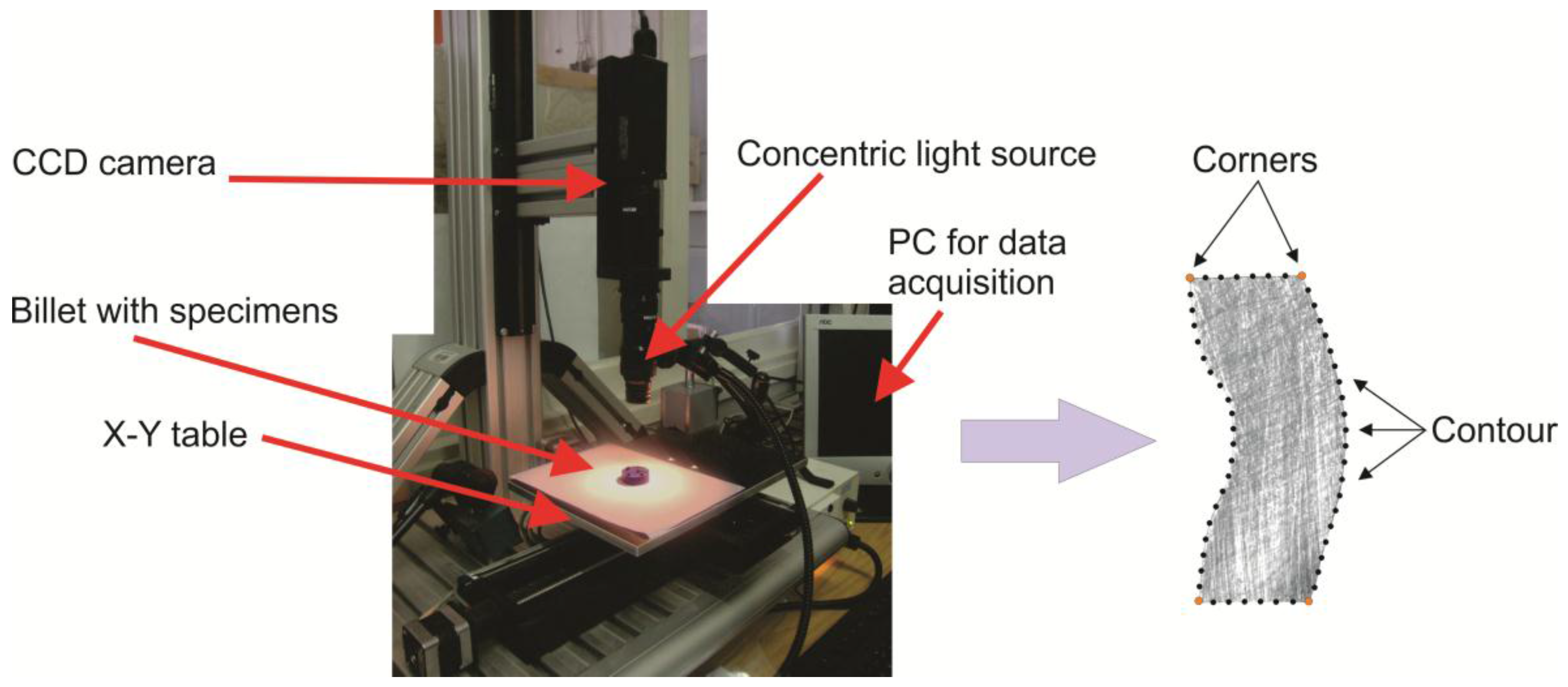
3.1. Experimental Work

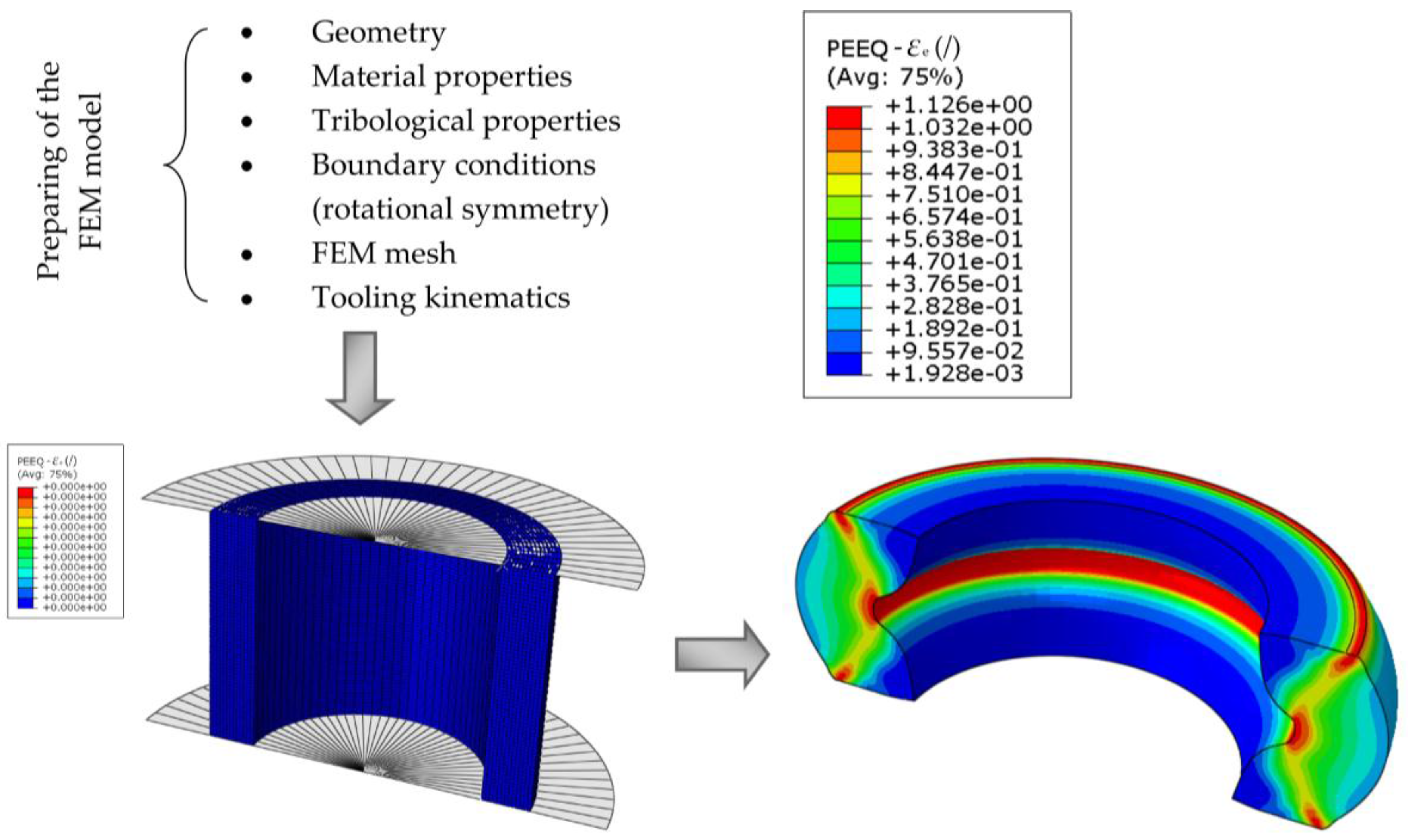
The upsetting of the tubular specimen was performed on a universal testing machine AMSLER (Zwick Roell AG, Ulm, Germany) with a nominal force of 300 kN. The forming force was measured with a 500 kN load cell with an accuracy of ±450 N while the displacement was acquired with an incremental transducer having an accuracy of ±0.01 mm. Load-stroke diagrams were obtained by using a specialized program for signal processing [24].

The specimens of the tube with a wall thickness of 2 mm and an initial height of 10 mm were upset up to the height of 5.81 ± 0.02 mm. This upsetting height represents a true equivalent strain of ε_e = 0.543. To minimize the friction between the tubular specimen and both tooling plates, the PTFE foil having a thickness of 0.2 mm was applied as a lubricant.

The experiments were performed with three samples. Their outer diameters were in the range of ±0.015 mm and inner diameters in the range of ±0.035 mm. The force-travel diagram used in further analyses represents the average value of all experiments. The standard deviation was in the range of ±2% for the whole range of force course.

After upsetting, the specimens were halved by wire electro-discharge machining (EDM) and sealed into a billet-shaped resin for their easier handling. To acquire the cross-sections of the specimens needed for their comparative evaluation with FEM results, they were scanned on the x-y table with a CCD camera. Concentric lighting was provided by a flexible optical fiber cable and a SCHOTT FOSTEC DCR III halogen light source.

Since the measuring equipment does not have a fix focus and magnification, it is necessary to calibrate it prior to measurements. Therefore, the measurement calliper with a thickness of 1.00 mm was scanned together with the cross-sections of the upset specimens. With the use of image processing [29], the acquired pictures were aligned according to the X-Y coordinate system and contour points were acquired for comparison with the FEM results as shown in Figure 1.

Friction represents an important factor in the shaping of a specimen in the upsetting process. Its influence increases with the size of the surfaces that are in contact during the forming process. This phenomenon is, in particular, necessary for bulk forming processes. However, in the case of axial compressive loading of a tubular specimen presented in the paper, it is assumed the only minor role of the friction coefficient on the tube shaping resulting from a small contact surface needs to be considered by a numerical method and statistical Taguchi approach.

The friction coefficient of the PTFE foil used in experimental work was determined with a standardized ring upsetting test [30,31]. According to the well-known diagram with calibration curves for various Coulomb’s friction coefficients μ the applied foil expressed a friction value between μ = 0.03 and μ = 0.04 [32]. Therefore, the evaluation of friction coefficient for analysis of variance (ANOVA) with the target value of μ = 0.035 was selected.

3.2. FEM Model

The upsetting process of the tubular specimens was analyzed with the ABAQUS commercial program [33] using the static implicit solver. Due to the axis-symmetric nature of the problem only a 2D-analysis with rotational symmetry was modelled (Figure 2). The FEM model consists of a deformable elastic-plastic specimen following Swift’s law [34] and analytical rigid tool parts. The analyzed cross-section was meshed with mapped FEM elements with a minimal 0.15 mm size. According to the initial size of the tested tubular specimen, the mesh consists of 952 (68 × 14) nodes and 871 (67 × 13) elements of the CAX4R type. The Coulomb friction model was used. Apart from the variation of the parameters of the flow curve yield stress R_p, material constant K, and hardening exponent n other material parameters used in the FEM model are as follows: density ρ = 7850 kg/m³, Young’s modulus E = 210 GPa, Poisson’s ratio ν = 0.3. According to the experiment, the bottom tool plate was fixed and the upper tool plate moved with a speed of 0.84 mm/s. The maximal tool displacement was 4.19 mm.

3.3. Design of Experiments

The Taguchi method is an engineering method for analyzing process parameters, which was developed by Genichi Taguchi. It can be used to obtain the relationship between the observed manufacturing process and its products [5,35]. The major advantage of the Taguchi method is the ability to analyze the observed process with a small number of experiments. It is a simple and systematic design of experiment tools, which is often used in statistically robust design [6,36,37].

In the presented paper, the Taguchi method was used to analyze the influence of the material parameters K, n, and R_p as well as the Coulomb’s friction coefficient μ on the forming force course and the final cross-sectional shape of the specimen. The parameters used in FEM simulations were based on the Taguchi method L₂₅ orthogonal array with four influential factors, in which each factor was presented on five levels.

3.4. Selection of Flow Curve Parameters

The analyzed tube is directly rolled from a steel strip to a corresponding diameter and welded with electrical resistance welding. After removing the outer welding burr and cooling the hollow sections are calibrated to precise, standardized dimensions [38]. Since the material is already pre-deformed, the use of the Swift flow curve approximation [34] was indispensable. The material description follows the equation:

σ_f = K·(ε₀ + ε_e)ⁿ

(1)

where K is a material constant, n is a hardening exponent, and ε₀ is the initial shift of the flow curve to obtain the yield stress R_p at a declared value of ε_e = 0.002. Since the yield stress is already pre-defined by the experiments, the value of ε₀ needs to be recalculated for each pair of parameters K and n in a reverse-engineering analysis. Digital analyses of upsetting the tubular specimens were performed with various flow curve parameters. The range of flow curve parameters was selected around the values known for sheet metal E420. Therefore, the hardening exponent n was selected in a range from 0.08 to 0.36 with an increment of 0.07. Similarly, the material constant K was increased from the lower value of 650 MPa to highest value of 950 MPa with an increment of 75 MPa. In order to analyze the influence of friction, the Coulomb’s friction coefficient in a wide range from μ = 0.025 to μ = 0.205 with an interval of 0.045 was selected.

Simulations were performed based on the combinations of the parameters K, n, R_p, and the friction coefficient μ using the Taguchi method designed on five levels as presented in

Table 2. Combinations of the analyzed parameters K, n, R_p, and μ.

Run	K (MPa)	n	μ	Rp (MPa)
1	875	0.15	0.205	544
2	800	0.29	0.025	544
3	725	0.08	0.070	544
4	725	0.36	0.025	482
5	875	0.08	0.160	482
6	725	0.29	0.205	420
7	875	0.36	0.115	420
8	950	0.36	0.160	544
9	800	0.15	0.160	420
10	650	0.08	0.025	420
11	875	0.22	0.025	606
12	950	0.29	0.115	482
13	800	0.22	0.205	482
14	950	0.15	0.025	668
15	800	0.36	0.070	606
16	875	0.29	0.070	668
17	725	0.22	0.160	668
18	950	0.22	0.070	420
19	725	0.15	0.115	606
20	650	0.15	0.070	482
21	650	0.36	0.205	668
22	950	0.08	0.205	606
23	800	0.08	0.115	668
24	650	0.22	0.115	544
25	650	0.29	0.160	606

.

3.5. Reverse Engineering Analyses

3.5.1. Determination of Impacts on Force Course

The influence of particular parameters K, n, R_p, and μ on the course of the forming force was analyzed at six points (Figure 3) defining different upsetting levels. The forces were labelled from F₁ to F₆ according to the tool displacement (

Table 3. Forces F₁ to F₆ and corresponding punch displacements.

Force	F1	F2	F3	F4	F5	F6
Punch displacement (mm)	0.81	1.56	2.27	3.03	3.63	4.19

).

According to the selected values of input parameters (marked with blue in

Table 4. FEM-obtained results of forming forces at six observed upsetting levels.

Run	K (MPa)	n	μ	Rp (MPa)	F1 (N)	F2 (N)	F3 (N)	F4 (N)	F5 (N)	F6 (N)
1	875	0.15	0.205	544	52,013.9	57,667.4	61,501.7	65,150.2	68,172.4	71,733.9
2	800	0.29	0.025	544	48,070.8	54,788.9	60,930.7	67,063.9	71,515.5	74,827.8
3	725	0.08	0.070	544	49,257.5	53,178.2	55,837.0	57,917.1	59,440.7	61,846.8
4	725	0.36	0.025	482	42,758.1	49,079.3	55,041.5	61,214.0	65,854.5	69,486.2
5	875	0.08	0.160	482	58,019.4	62,889.6	65,688.6	68,557.7	70,986.6	74,079.4
6	725	0.29	0.205	420	38,823.6	43,810.6	47,659.2	51,606.0	54,556.6	58,316.9
7	875	0.36	0.115	420	40,992.9	48,051.7	53,793.0	58,884.1	62,920.8	67,032.1
8	950	0.36	0.160	544	49,854.3	56,461.3	61,609.5	66,960.9	71,398.8	76,122.9
9	800	0.15	0.160	420	45,863.7	51,842.5	55,513.1	59,048.3	61,689.6	65,109.1
10	650	0.08	0.025	420	43,696.8	49,466.9	53,833.5	57,573.6	59,947.5	61,672.4
11	875	0.22	0.025	606	53,589.7	60,779.8	67,085.8	73,115.2	77,301.8	80,216.2
12	950	0.29	0.115	482	47,082.9	54,585.2	60,388.8	65,400.8	69,326.3	73,664.8
13	800	0.22	0.205	482	44,789.6	50,128.1	54,054.1	57,945.9	60,952.4	64,679.8
14	950	0.15	0.025	668	59,841.7	67,722.7	74,213.1	80,042.6	83,868.8	86,386.5
15	800	0.36	0.070	606	52,119.6	56,866.0	61,004.7	64,918.9	67,762.6	71,292.2
16	875	0.29	0.070	668	57,155.3	61,971.5	66,059.0	69,813.1	72,621.1	76,237.1
17	725	0.22	0.160	668	55,097.5	57,786.2	59,761.4	62,460.3	64,831.4	67,962.0
18	950	0.22	0.070	420	47,639.9	56,792.6	63,388.5	68,961.5	72,364.8	76,387.3
19	725	0.15	0.115	606	50,630.8	53,535.3	55,744.4	57,895.8	60,194.2	62,855.8
20	650	0.15	0.070	482	41,969.5	45,564.2	48,332.2	50,705.5	52,254.3	54,802.9
21	650	0.36	0.205	668	55,220.8	58,087.2	60,476.3	63,201.4	66,029.6	69,445.6
22	950	0.08	0.205	606	63,122.5	68,155.2	71,328.3	74,207.3	76,963.0	80,346.5
23	800	0.08	0.115	668	56,356.8	59,488.8	61,629.4	63,646.8	65,855.6	68,638.0
24	650	0.22	0.115	544	45,540.9	48,365.2	50,623.7	52,847.7	55,144.8	57,802.9
25	650	0.29	0.160	606	50,234.4	52,973.6	55,071.0	57,648.8	60,236.6	63,319.4

) following the Taguchi L₂₅ matrix, the FEM simulations were performed. Forces F₁ to F₆ were extracted from each analysis (Table 4).

Using the ANOVA concept, the influences of the parameters K, n, R_p, and μ, as well as their two-factor products on particular observed force states were studied, and response surface was determined. As a measure of parameter importance the F-test was performed. The significance of a particular parameter was analyzed with the level of “p-value” below 5%, marked with green fields in

Table 5. The influence of the parameters K, n, R_p, and μ, and their products on different levels of upsetting force.

Force	Influential Parameter	p-Value	Force	Influential Parameter	p-Value
F1	K	<0.0001	F4	K	<0.0001
	n	0.0003		n	0.6672
	μ	0.4553		μ	0.0021
	Rp	<0.0001		Rp	<0.0001
	K·n	0.0091		K∙n	0.0033
	K∙μ	0.1899		K∙μ	0.8832
	K∙Rp	0.2535		K∙Rp	0.4999
	n∙μ	0.3473		n∙μ	0.2916
	n∙Rp	0.0007		n∙Rp	0.0019
	μ∙Rp	0.7288		μ∙Rp	0.3103
F2	K	<0.0001	F5	K	<0.0001
	n	0.0002		n	0.4014
	μ	0.0496		μ	0.0053
	Rp	<0.0001		Rp	0.0009
	K∙n	0.0014		K∙n	0.0093
	K∙μ	0.3163		K∙μ	0.8549
	K∙Rp	0.5220		K∙Rp	0.5320
	n∙μ	0.2142		n∙μ	0.3447
	n∙Rp	<0.0001		n∙Rp	0.0180
	μ∙Rp	0.7476		μ∙Rp	0.3900
F3	K	<0.0001	F6	K	<0.0001
	n	0.0079		n	0.1046
	μ	0.0015		μ	0.0096
	Rp	<0.0001		Rp	0.0011
	K∙n	0.0005		K∙n	0.0103
	K∙μ	0.5451		K∙μ	0.8752
	K∙Rp	0.8954		K∙Rp	0.5490
	n∙μ	0.1529		n∙μ	0.3933
	n∙Rp	<0.0001		n∙Rp	0.0178
	μ∙Rp	0.3630		μ∙Rp	0.3572

. It can be found that parameter significance varies at different levels of forming force F₁ to F₆.

It can be observed that the material parameter K is influential at the forces of all six upsetting states, whereas the parameter n is significant only in the first three force states. The influence of the material parameter R_p is significant in all six states, but its influence decreases at the last two states. The Coulomb’s friction coefficient μ does not have a significant influence on the first force state; however, from the second to the third stated its influence increases, and then from the fourth to the last force state it decreases again, although its influence is still significant. This shows an important tribological influence on the force-travel course despite the relatively small contact surface of the compressed ring specimen.

With all six force states, F₁ to F₆, the influences of the products K∙n and n∙R_p have also been shown as significant (Table 5).

The performed ANOVA delivers the following equations for the upsetting forces F₁ to F₆:

F₁ = −34162.0622 + 99.6195·K + 48825.3664·n − 1.8503 × 10⁵·μ + 95.7931·R_p − 207.8010·K·n + 223.4257·K·μ − 0.09234·K·R_p + 1.1618 × 10⁵∙n·μ + 159.8426∙n∙R_p − 47.7240·μ·R_p

(2)

F₂ = −15468.8308 + 99.0229∙K + 59024.9262∙n − 1.7275 × 10⁵∙μ + 32.4871∙R_p − 221.9004∙K∙n + 137.4341·K·μ − 0.04152∙K∙R_p + 1.2678 × 10⁵∙n·μ + 164.3933∙n∙R_p + 36.1033∙μ∙R_p

(3)

F₃ = 1312.5867 + 92.6784∙K + 81515.0248∙n − 1.7325 × 10⁵∙μ − 20.6423∙R_p − 239.3537∙K∙n + 78.0233∙K∙μ + 8.0487 × 10⁻³·K·R_p + 1.4007 × 10⁵∙n∙μ + 156.5391∙n∙R_p + 98.3775∙μ∙R_p

(4)

F₄ = 17650.5047 + 83.9019∙K + 1.0640 × 10⁵∙n − 1.6851 × 10⁵∙μ − 71.0559∙R_p − 257.9681∙K∙n + 25.8374∙K∙μ + 0.05715∙K∙R_p + 1.3937 × 10⁵∙n∙μ + 151.2000∙n∙R_p + 151.1420∙μ∙R_p

(5)

F₅ = 18349.3973 + 86.2074∙K + 1.3793 × 10⁵∙n − 1.9589 × 10⁵∙μ − 79.2528∙R_p − 282.2140∙K∙n + 41.1800∙K∙μ + 0.06773∙K∙R_p + 1.5928 × 10⁵∙n·μ + 135.6569∙n∙R_p + 163.1456∙μ∙R_p

(6)

F₆ = 17679.0298 + 89.9239∙K + 1.3678 × 10⁵∙n − 1.8654 × 10⁵∙μ − 77.5335∙R_p − 271.1428∙K∙n + 34.6087∙K∙μ + 0.06350∙K∙R_p + 1.4032 × 10⁵∙n∙μ + 133.0687∙n∙R_p + 171.2837∙μ∙R_p

(7)

The obtained influential equations of forming forces F₁ to F₆ represent the basis for the determination of flow curve parameters when they are compared with experimentally obtained values.

3.5.2. Multi-Parameter Analysis for an Inverse-Engineering Approach

The reverse engineering approach of flow curve determination is based on multi-parameter optimization based on equations F₁ to F₆ (Equations (2)–(7)). The range for particular input parameters can be narrowed down to the experimentally expected range. The real experiment of the tube compression was compared with corresponding FEM analysis. For FEM simulation input data based on the multi-functional parameter determination having the material properties described in Section 2 were selected. Through this, the value of yield stress R_p is fixed to 572 MPa. In the ANOVA it was observed that the initial assumption of the negligible influence of friction coefficient was wrong. Therefore, the proper selection of friction coefficient needs to be considered in further analysis. Values between μ = 0.03 and μ = 0.04 are selected according to the friction measurement of PTFE foil from the literature [32]. Through this, the unknown parameters are limited to flow curve parameters K and n only. The multifunctional analysis can be solved analytically or graphically. However, the analytical determination delivers more accurate results and was therefore selected as a preferred solution. The graphical solution would be used only in the case of the unsolvable analytic solution. The experimentally obtained target values of F₁ to F₆ are presented in

Table 6. Experimentally obtained values of F₁ to F₆.

Punch Displacement (mm)	Force (N)
0.81	49,537
1.56	54,600
2.27	58,687
3.03	61,612
3.63	63,225
4.19	64,838

.

To perform the multifunctional analysis, the spread range for each experimentally determined force F₁ to F₆ is to examine the procedure used for determination of K, n, and μ was based on the spread of F₁ in the 4% range, and F₂ to F₆ in the range of 2% according to the experimentally obtained values. The analytical, multifunctional optimization of all six target equations (Equations (2)–(7)) finally delivers four different values of K and n as presented in

Table 7. Determined combination of material parameters and friction coefficient μ.

Number	K (MPa)	n	μ	Rp(MPa)	ε0
1	713.0	0.195	0.035	572	0.321
2	716.7	0.187	0.039	572	0.298
3	710.0	0.203	0.033	572	0.343
4	708.4	0.199	0.031	572	0.339

. Despite that, all four results in Table 7 fit the prescribed criteria of the multifunctional analysis; the solution in the first row is the most optimal result since the used ANOVA optimization delivers the best solution first.

The value of constant ε₀ is calculated from

$${\mathsf{\epsilon }}_0={\left(\frac{R_{\mathrm{p}}}{K}\right)}^{\frac{1}{n}}-0.002$$

(8)

The obtained values of flow curve parameters were inserted into the FEM model, and the upsetting process in a digital environment was re-run. The FEM simulation was re-run with the material parameters following the Swift equation according to the case number 1 from the Table 7:

σ_f = 713·(0.321 + ε_e)^0.195

(9)

Comparison of experimental and FEM predicted force course during the upsetting process together with their differences are presented in Figure 4. The differences are in a close range lying below the 5% limit.

3.6. Comparison of Tube Shaping

Determination of flow curves by the reverse engineering method led to the quality determination of the force-travel course of the upset specimens. However, it is necessary to prove whether the specimens with the Taguchi method, ANOVA, multifunctional optimization, and FEM determined material parameters are in fact shaped in the same manner as the experimental ones.

In addition to the evaluation of forming force F versus punch displacement, the specimen shape was observed. This research analyzed the specimen shape at various compression states for the determination of material parameters K, n, and R_p. The simulated variation of material parameters was first selected according to Equation (9) and analyzed for three different values of the Coulomb’s friction coefficient: μ = 0.035, μ = 0.045, and μ = 0.15. The influence of material parameters on the specimen shape was also analyzed with 50% higher material parameters than those determined in Equation (9):

σ_f = 1070·(0.468 + ε_e)^0.29

(10)

Figure 5 shows that the friction coefficient has a measurable influence on part shaping. According to FEM simulation, the changes of the shape (diameter) are indeed minor regarding the material parameters and they are for the specimens having diameter of 13.93 mm in the range below ±0.05 mm. Based on this information, it was concluded that the determination of material parameters is significantly more reliable and accurate according to the analysis of the forming force.

To obtain comparative contour data of the upset tubular specimen acquired by the CCD camera as presented in Figure 1 and matched with final FEM results, a specialized program was written [24]. The contour-recognition program orients the specimen according to the x-y axis, compares the evaluated sample with the scanned calibre of 1.00 mm, takes out the contour points of the specimen, and compares them with the coordinates of the FEM mesh extracted from the nodes after the simulation.

As is evident from Figure 6, the specimen correlates well with the FEM results for the observed specimen height at the end of the forming process. However, minor discrepancies between the upset specimens and FEM results can be observed at the inner contour of the specimen and upper part of the outer bulged specimen’s area. These differences are not significant; however, influential parameters on part shaping are to analyze more into the detail in the future. Currently, in FEM simulations only the fixed value of friction coefficient μ was considered. In particular, the influence of the friction coefficient during the process is to study in order to evaluate its influence on the part shaping.

4. Conclusions

In this paper, the determination of a flow curve for thin-walled tubular specimens was implemented. The analyses were based on a modified upsetting test of tubular specimens with a D/t ratio of 7. Using the Taguchi method and analysis of variance (ANOVA), the material’s flow curve parameters were determined. The main conclusions are the following:

1)

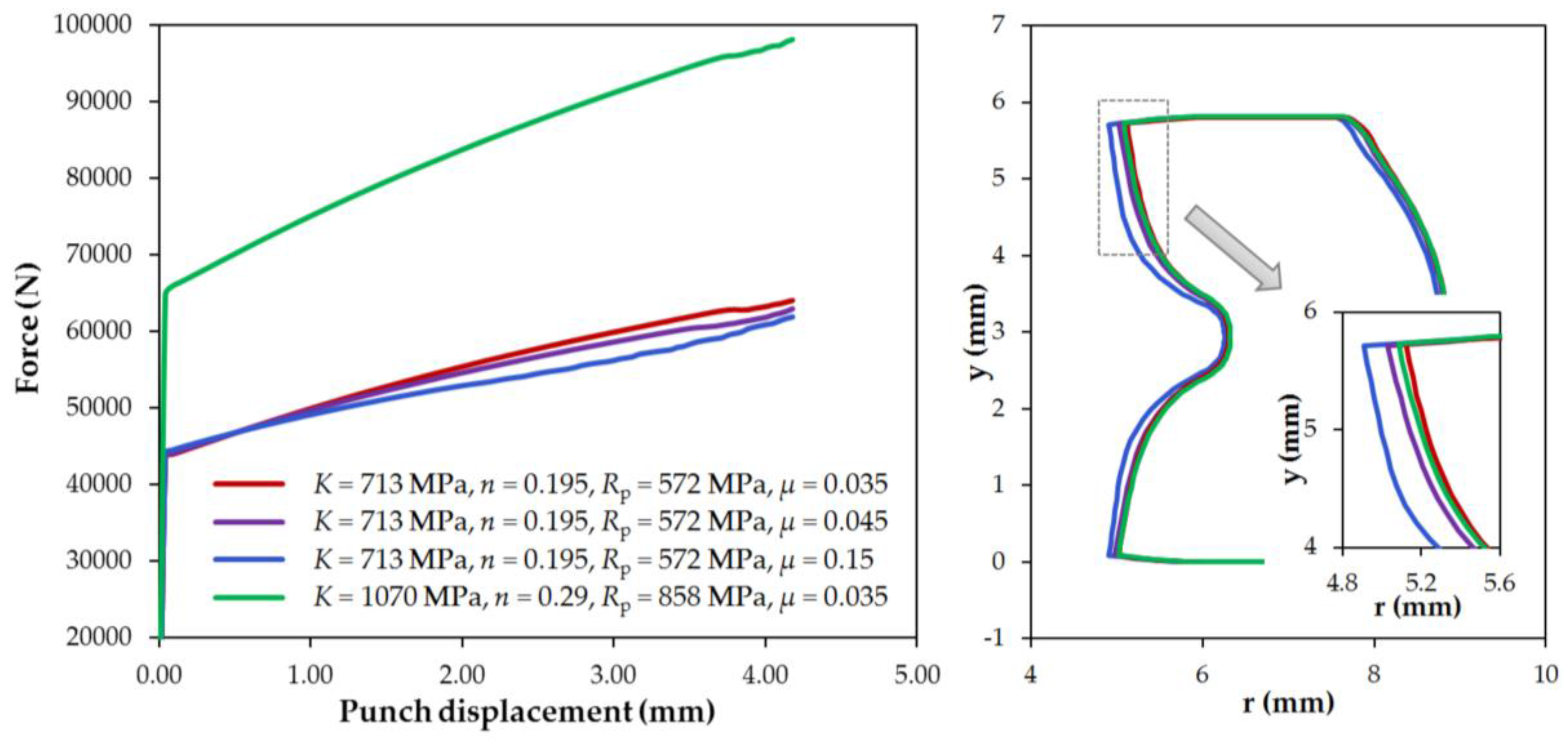
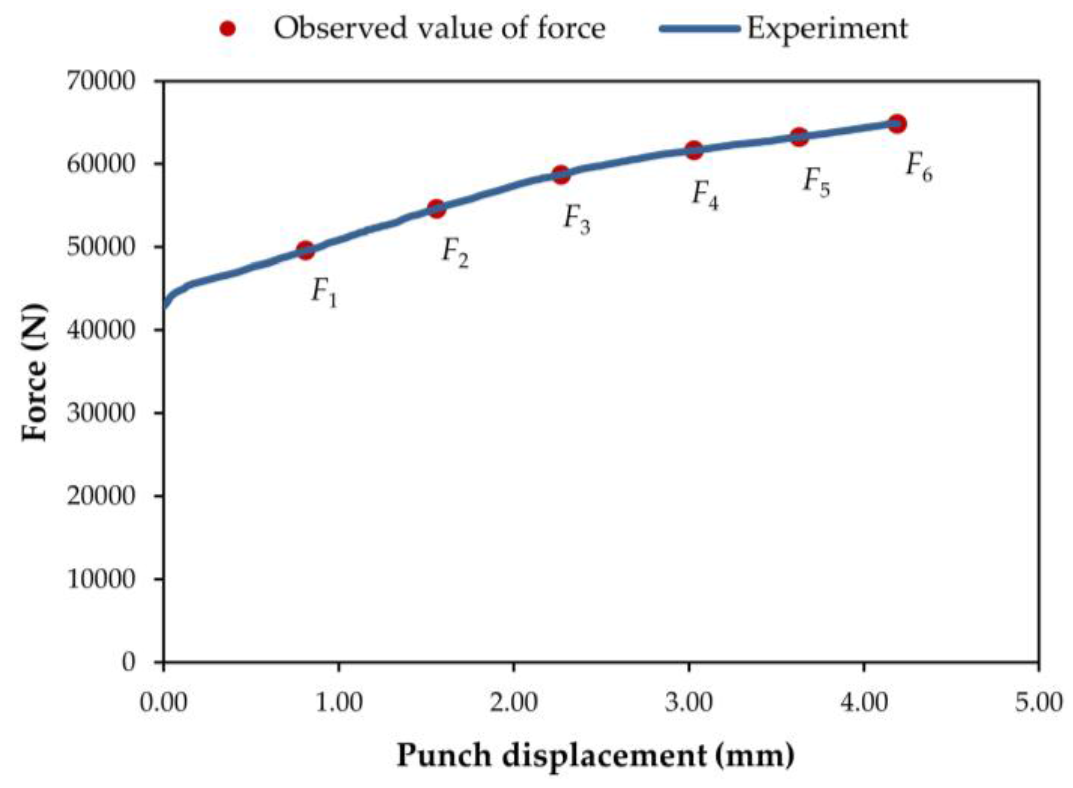
The forming force versus punch displacement was used for a reverse engineering approach to determine the flow curve parameters since it was found that the variation of material parameters has only a minor role on the specimen shaping.

2)

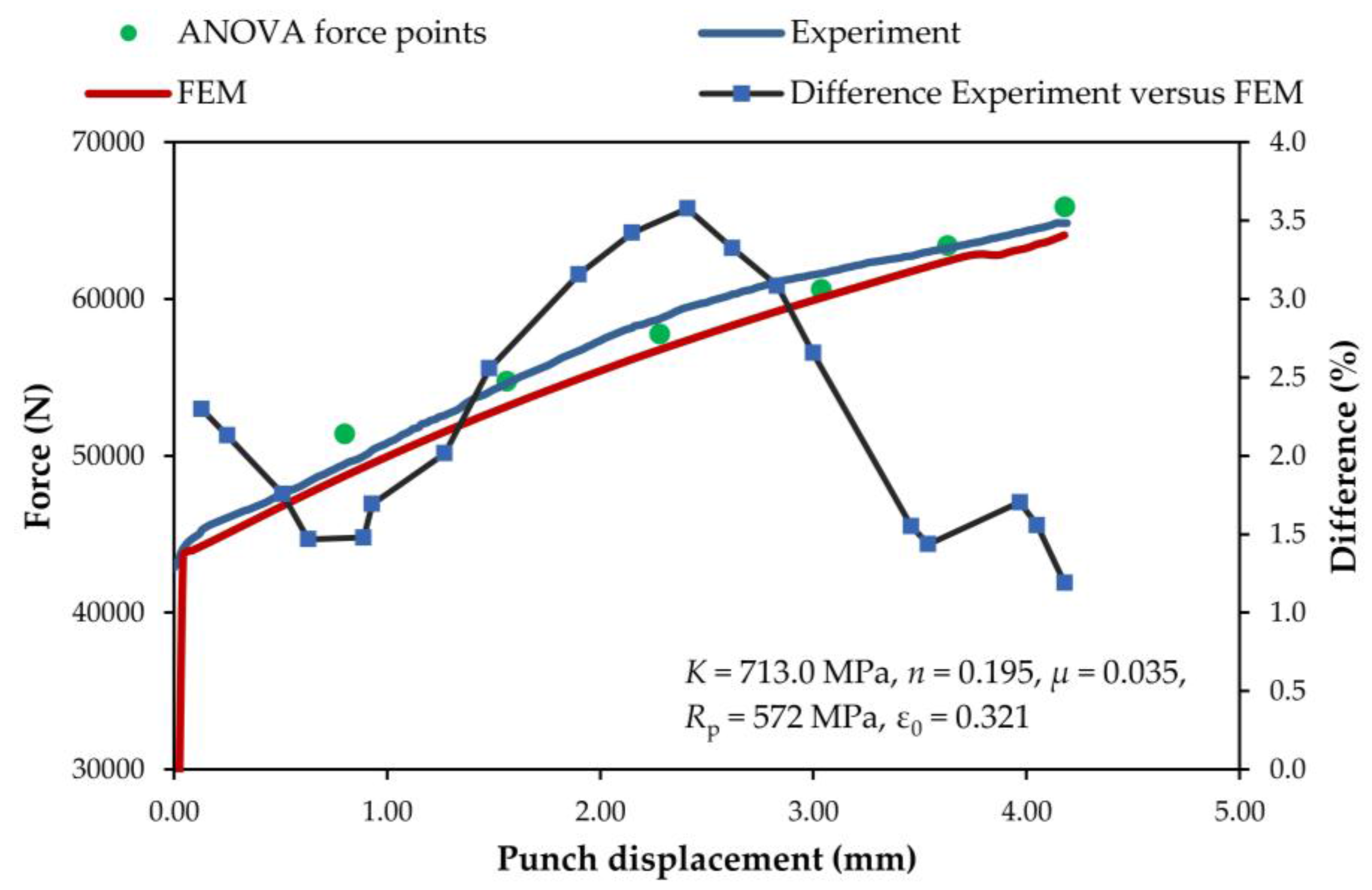
The optimization approach based on the comparison of experimentally and statistically determined values (Taguchi + ANOVA) of forming force at six upsetting levels delivered the parameters of the material’s flow curve K = 713 MPa, n = 0.195, and ε₀ = 0.321 according to Swift’s power law. The friction coefficient μ in this optimization was selected according to the one measured for the PTFE foil. The yield stress of the tube R_p was also determined experimentally.

3)

The comparison of the FEM-predicted force course based on the determined material flow curve and the experimental force course showed that the differences are below 5%.

4)

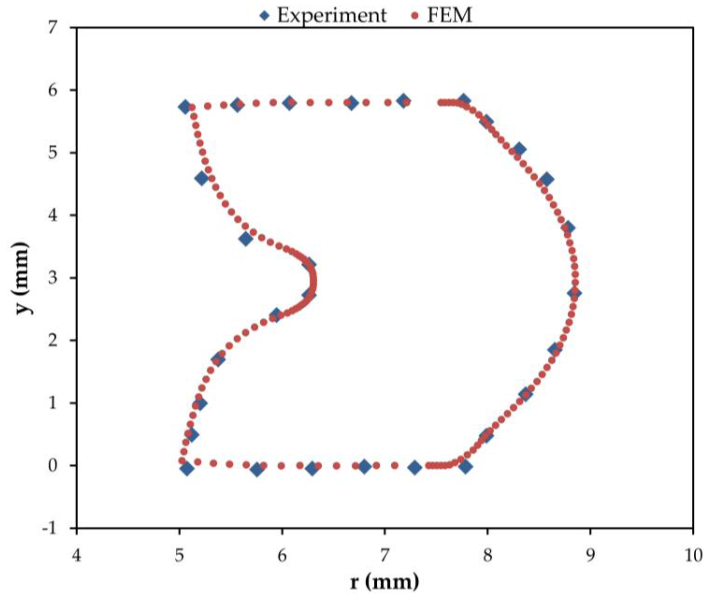
The comparison of the cross-sectional contours of the upset specimens with the numerically obtained results for the determined flow curve according to Swift’s law showed only minor shape deviations.

5)

Future analyses should focus on the geometrical optimization of the specimens regarding the d₀:h₀ ratio for various D/t ratios. The presented methodology needs to be further tested regarding its robustness according to all input parameters, such as the level of the flow curve, the value of R_p, and the friction coefficient.

References

1. Gu, G.; Xia, Y.; Zhou, Q. On the fracture possibility of thin-walled tubes under axial crushing. Thin Walled Struct. 2012, 55, 85–95. [Google Scholar] [CrossRef]
2. He, Z.; Yuan, S.; Liu, G.; Wu, J.; Cha, W. Formability testing of AZ31B magnesium alloy tube at elevated temperature. J. Mater. Process. Technol. 2010, 210, 877–884. [Google Scholar] [CrossRef]
3. Shim, D.-S.; Kim, K.-P.; Lee, K.-Y. Double-stage forming using critical pre-bending radius in roll bending of pipe with rectangular cross-section. J. Mater. Process. Technol. 2016, 236, 189–203. [Google Scholar] [CrossRef]
4. Alves, L.M.; Martins, P.A.F. Forming of thin-walled tubes into toroidal shells. J. Mater. Process. Technol. 2010, 210, 689–695. [Google Scholar] [CrossRef]
5. Souissi, N.; Souissi, S.; Niniven, C.L.; Amar, M.B.; Bradai, C.; Elhalouani, F. Optimization of Squeeze Casting Parameters for 2017 A Wrought Al Alloy Using Taguchi Method. Metals 2014, 4, 141–154. [Google Scholar] [CrossRef]
6. Zeng, G.; Lai, X.; Yu, Z.; Lin, Z. Numerical Simulation and Sensitivity Analysis of Parameters for Multistand Roll Forming of Channel Section With Outer Edge. J. Iron Steel Res. Int. 2009, 16, 32–37. [Google Scholar] [CrossRef]
7. Celentano, D.J.; Rosales, D.A.; Peña, J.A. Simulation and Experimental Validation of Tube Sinking Drawing Processes. Mater. Manuf. Process. 2011, 26, 770–780. [Google Scholar] [CrossRef]
8. Brnic, J.; Niu, J.; Canadija, M.; Turkalj, G.; Lanc, D. Behavior of AISI 316L Steel Subjected to Uniaxial State of Stress at Elevated Temperatures. J. Mater. Sci. Technol. 2009, 25, 175–180. [Google Scholar]
9. Brnic, J.; Turkalj, G.; Canadija, M.; Lanc, D.; Krscanski, S.; Brcic, M.; Li, Q.; Niu, J. Mechanical Properties, Short Time Creep, and Fatigue of an Austenitic Steel. Materials 2016, 9, 298. [Google Scholar] [CrossRef]
10. Vukelic, G.; Brnic, J. Predicted Fracture Behavior of Shaft Steels with Improved Corrosion Resistance. Metals 2016, 6, 40. [Google Scholar] [CrossRef]
11. Geiger, M.; Hußnätter, W.; Merklein, M. Specimen for a novel concept of the biaxial tension test. J. Mater. Process. Technol. 2005, 167, 177–183. [Google Scholar] [CrossRef]
12. Suttner, S.; Merklein, M. Experimental and numerical investigation of a strain rate controlled hydraulic bulge test of sheet metal. J. Mater. Process. Technol. 2016, 235, 121–133. [Google Scholar] [CrossRef]
13. Cao, Z.; Wang, F.; Wan, Q.; Zhang, Z.; Jin, L.; Dong, J. Microstructure and mechanical properties of AZ80 magnesium alloy tube fabricated by hot flow forming. Mater. Des. 2015, 67, 64–71. [Google Scholar] [CrossRef]
14. Wang, H.; Bouchard, R.; Eagleson, R.; Martin, P.; Tyson, W. Ring Hoop Tension Test (RHTT): A Test for Transverse Tensile Properties of Tubular Materials. J. Test. Eval. 2002, 30, 382–391. [Google Scholar] [CrossRef]
15. Lin, Y.; He, Z.; Yuan, S.; Wu, J. Formability determination of AZ31B tube for IHPF process at elevated temperature. Trans. Nonferr. Met. Soc. China 2011, 21, 851–856. [Google Scholar] [CrossRef]
16. Faraji, G.; Hashemi, R.; Mashhadi, M.M.; Dizaji, A.F.; Norouzifard, V. Hydroforming Limits in Metal Bellows Forming Process. Mater. Manuf. Process. 2010, 25, 1413–1417. [Google Scholar] [CrossRef]
17. Song, W.-J.; Heo, S.-C.; Ku, T.-W.; Kim, J.; Kang, B.-S. Evaluation of effect of flow stress characteristics of tubular material on forming limit in tube hydroforming process. Int. J. Mach. Tools Manuf. 2010, 50, 753–764. [Google Scholar] [CrossRef]
18. Agüero, A.; Pallarés, F.J.; Pallarés, L. Equivalent geometric imperfection definition in steel structures sensitive to lateral torsional buckling due to bending moment. Eng. Struct. 2015, 96, 41–55. [Google Scholar] [CrossRef]
19. Liu, N.; Yang, H.; Li, H.; Tao, Z.; Hu, X. An imperfection-based perturbation method for plastic wrinkling prediction in tube bending under multi-die constraints. Int. J. Mech. Sci. 2015, 98, 178–194. [Google Scholar] [CrossRef]
20. Liu, N.; Yang, H.; Li, H.; Zhan, M.; Tao, Z.; Hu, X. Modelling of Wrinkling in NC Bending of Thin-walled Tubes with Large Diameters under Multi-die Constraints Using Hybrid Method. Proced. Eng. 2014, 81, 2171–2176. [Google Scholar] [CrossRef]
21. Guillow, S.R.; Lu, G.; Grzebieta, R.H. Quasi-static axial compression of thin-walled circular aluminium tubes. Int. J. Mech. Sci. 2001, 43, 2103–2123. [Google Scholar] [CrossRef]
22. Peek, R. Wrinkling of tubes in bending from finite strain three-dimensional continuum theory. Int. J. Solids Struct. 2002, 39, 709–723. [Google Scholar] [CrossRef]
23. Lee, K.-L.; Pan, W.-F.; Kuo, J.-N. The influence of the diameter-to-thickness ratio on the stability of circular tubes under cyclic bending. Int. J. Solids Struct. 2001, 38, 2401–2413. [Google Scholar] [CrossRef]
24. Pirh, T. Določevanje Preoblikovalnih Lastnosti Cevastih Preizkušancev (Determination Forming Properties of Tube Specimens). Master’s Thesis, University of Ljubljana, Ljubljana, Slovenia, May 2010. [Google Scholar]
25. Bunge, H.J.; Pöhlandt, K.; Tekkaya, A.E.; Banabic, D. Formability of Metallic Materials: Plastic Anisotropy, Formability Testing, Forming Limits, 1st ed.; Springer-Verlag Berlin Heidelberg: Berlin, Germany, 2000. [Google Scholar]
26. Schey, J.A. Tribology in Metalworking: Friction, Lubrication and Wear; American Society for Metals: Metals Park, OH, USA, 1983. [Google Scholar]
27. Camacho, A.M.; Veganzones, M.; Claver, J.; Martín, F.; Sevilla, L.; Sebastián, M.Á. Determination of Actual Friction Factors in Metal Forming under Heavy Loaded Regimes Combining Experimental and Numerical Analysis. Materials 2016, 9, 751. [Google Scholar] [CrossRef]
28. Sofuoglu, H.; Rasty, J. On the measurement of friction coefficient utilizing the ring compression test. Tribol. Int. 1999, 32, 327–335. [Google Scholar] [CrossRef]
29. Pipan, M.; Kos, A.; Herakovic, N. Adaptive Algorithm for the Quality Control of Braided Sleeving. Adv. Mech. Eng. 2014, 6, 1–8. [Google Scholar] [CrossRef]
30. Hsia, S.-Y.; Shih, P.-Y. Wear Improvement of Tools in the Cold Forging Process for Long Hex Flange Nuts. Materials 2015, 8, 6640–6657. [Google Scholar] [CrossRef]
31. Altan, T.; Ngaile, G.; Shen, G. Cold and Hot Forging: Fundamentals and Applications, 1st ed.; ASM International: Materials Park, OH, USA, 2005; pp. 295–298. [Google Scholar]
32. Pepelnjak, T. Analyses of friction coefficients of PTFE foils used for forming applications at elevated temperatures. In Proceedings of the IN-TECH 2015—International Conference on Innovative Technologies, Dubrovnik, Croatia, 9 November 2015; pp. 438–441.
33. Abaqus Theory Manual, version 6.14; Software of Dassault Systems; Dassault Simulia Company: Providence, RI, USA, 2016.
34. Gronostajski, Z. The constitutive equations for FEM analysis. J. Mater. Process. Technol. 2000, 106, 40–44. [Google Scholar] [CrossRef]
35. Lin, J.-C.; Lee, K. Optimization of Bending Process Parameters for Seamless Tubes Using Taguchi Method and Finite Element Method. Adv. Mater. Sci. Eng. 2015, 2015, 8. [Google Scholar] [CrossRef]
36. Abedini, A.; Rahimlou, P.; Asiabi, T.; Ahmadi, S.R.; Azdast, T. Effect of flow forming on mechanical properties of high density polyethylene pipes. J. Manuf. Process. 2015, 19, 155–162. [Google Scholar] [CrossRef]
37. Gürün, H.; Karaağaç, İ. The Experimental Investigation of Effects of Multiple Parameters on the Formability of the DC01 Sheet Metal. Stroj. Vestn. J. Mech. Eng. 2015, 61, 651–662. [Google Scholar] [CrossRef]
38. Steel Tubes for Precision Applications—Technical Delivery Conditions—Part 5: Welded and Cold Sized Square and Rectangular Tubes, British Standard, BS EN 10305-5:2003. Available online: http://www.lincsourcing.fr/admin/bildbank/uploads/Dokument/Body_of_knowledge/British_standard,_steel_tubes_for_precision_applications.pdf (accessed on 15 July 2016).
Figure 1. Acquisition of the specimen contour by a CCD camera.
Metals 06 00257 g001
Figure 2. Rotational-symmetric FEM model of the tube (left) in a 3D-view and the results of the equivalent strain distribution obtained by a FEM simulation in a 3D-view (right).
Metals 06 00257 g002
Figure 3. Force—travel diagram.
Metals 06 00257 g003
Figure 4. Comparison of force course for selected material parameters from Table 7.
Metals 06 00257 g004
Figure 5. Influence of the material parameters and friction coefficient on the forming force (left) and specimen shape (right).
Metals 06 00257 g005
Figure 6. Comparison between the part shape and FEM results obtained by multi-parameter optimization.
Metals 06 00257 g006