Study on Austenitization Kinetics of SA508 Gr.3 Steel Based on Isoconversional Method

Abstract

The austenitization kinetics of SA508 Gr.3 steel during heating was studied using the isoconversional method combined with continuous thermal dilatometric tests for the first time. The model-free austenitization kinetics was built and the effective activation energy as a function of transformed austenite fraction was determined without transformation models. Then, the corresponding regression validation was carried out. The time-temperature-austenitization (TTA) diagram of SA508 Gr.3 steel, which is very difficult to be obtained using experiment measures, was constructed. Finally, the austenitization kinetics in a more realistic case, i.e., under non-constant heating rates, was predicted, which is found to agree well with the experimental results.

1. Introduction

Austenitization is an important solid-state phase transformation involved in almost all of the hot-working processes of steels, such as heat treatment, welding, surface cladding, forging, etc. In recent years, several quantitative models have been proposed to describe the austenitization kinetics during heating, which were all based on the Johnson-Mehl-Avrami-Kolmogorov (JMAK) equation [1]:

α = 1 – exp[−(k(T)t)ⁿ]

(1)

where α represents the transformed austenite fraction, k(T) and n are the parameters depending on temperature T. With the aid of the nucleation and growth functions reported by Roosz et al. [2], different models describing the kinetics of austenite formation from different initial microstructures (pearlite, ferrite, bainite, martensite, or their mixtures) during heating were developed. Garcíia de Andrés et al. [3] derived a mathematical model of the pearlite-austenite transformation during continuous heating in a eutectoid steel with a fully pearlitic initial microstructure. Caballero et al. [4] presented a model to describe the ferrite-austenite transformation in Armco iron and three low-carbon/low-manganese steels starting with a fully ferritic initial microstructure. This model can be used to calculate the volume fractions of austenite and ferrite during transformation as a function of temperature. Caballero et al. [5] used theoretical knowledge regarding the isothermal formation of austenite from pure and mixed initial microstructures to develop a model for the non-isothermal austenite formation in a wide range of steels with an initial microstructure consisting of ferrite and/or pearlite. In addition to the initial microstructures, more details of some other factors were also taken into account in the study of austenitization kinetics. Gaude-Fugarolas and Bhadeshia [6] suggested a model that considered the effect of various factors, such as the steel composition, grain size, pearlite interlamellar spacing, and heating rate. Surm et al. [7] investigated the effect of heating rate on austenitization kinetics and modeled the austenitization with non-constant heating rate in hypereutectoid steels.

The dilatometric testing has long been employed in transformation kinetics investigation, which collects the information of diameter or length change of a sample during isothermal or continuous thermal process. In isothermal dilatometric testing, the transformation is usually expected to be fulfilled completely so that the kinetics information can be collected, but the limitation is also obvious as it is very difficult to keep the whole transformation process in an isothemal condition. For example, the austenitization process of some steels can be finished in very short period, i.e., tens of second, or even several second, making transformation starts during the heating-up stage and only part of the transformation happens under isothermal condition [8,9]. From this point of view, the continuous thermal dilatometry technique is an alternative method. In addition, it is worth mentioning that some new methods have been used for austenite formation study recent years. For example, Savran et al. [10] studied the nucleation and growth of austenite from ferrite/pearlite structures using a three-dimensional high-energy X-ray diffraction (3-D XRD) microscope. Additionally, Esin et al. [11] investigated the austenitization during both slow and fast heating for different microstructures of a selected low-alloy steel by simultaneously using in situ high-energy synchrotron X-ray diffraction and dilatometry.

The isoconversional method, namely “model-free” method, which is derived from the isoconversional principle [12], can evaluate the dependence of the effective activation energy on the degree of conversion without any assumption on the conversion mechanism. Since not making use of any approximations about transformation models, this method would potentially be more accurate and might avoid the risk due to wrong model assumptions. An important advantage of the isoconversional method is that it is possible to correctly and easily describe the kinetics of complex conversions in model-free way, i.e., model-free kinetics.

A large number of isoconversional methods has been constructed, such as Flynn-Wall-Ozawa (FWO) Method [13,14], Kissinger-Akahira-Sunose (KAS) Method [15,16], Vyazovkin’s Advanced Isoconversional (VA) Method [17], etc. The most commonly used isoconversional method is the differential isoconversional method of Friedman, namely Friedman method [18,19].

This method has widely been used in the field of thermal analysis, but in very few studies of the solid-state phase transformation kinetics of metals, for example, aluminum alloys [20], hypo-eutectoid Cu-Al alloys [21], and Cu-Al-Mn alloys [22]. In this work, we tried to use, for the first time, the isoconversional method to investigate the austenitization kinetics of a hypo-eutectoid steel, based on the data collected from the continuous thermal dilatometric experiments.

2. Theoretical Background and Experimental Procedures

2.1. General Equation for Kinetics

Measurement and parameterization of the phase transformation rate is one of the focused subjects in modern kinetic theory. For solid-state phase transformations, e.g., austenitization, the transformation rate is expressed by the equation below [23,24]:

$$\frac{\text{d}\mathsf{\alpha }}{\text{d}t}=k(T)f(\mathsf{\alpha })=A\exp \left(\frac{-E}{RT}\right)f(\mathsf{\alpha })$$

(2)

where k(T) is the rate constant which represents the temperature dependence of the transformation rate and can be described by Arrhenius Equation k(T) = Aexp(−E/RT), f(α) indicates the transformation model, A is the pre-exponential factor, E denotes the effective activation energy, and R is the universal gas constant (8.314 J/mol·K).

For the linear non-isothermal condition, Equation (2) is frequently used in the form of [10]:

$$\mathsf{\beta }\frac{\text{d}\mathsf{\alpha }}{\text{d}t}=A\exp \left(\frac{-E}{RT}\right)f(\mathsf{\alpha })$$

(3)

where β is the heating rate.

2.2. JMAK Equation

Equation (2) is a general equation of kinetic theory and can be used to describe different conversion processes with different explicit expressions of f(α) [25]. The JMAK equation can be translated into Equation (2). Taking logarithmic derivative of Equation (1) leads to:

$$\frac{\text{d}\mathsf{\alpha }}{\text{d}t}=nk{(T)}^n{t}^{n-1}(1-\mathsf{\alpha })$$

(4)

$$t^{n-1}=k{(T)}^{(1-n)}\ln {\left(\frac{1}{1-\mathsf{\alpha }}\right)}^{\frac{n-1}{n}}$$

(5)

Substituting Equation (5) into Equation (4), and making simple rearrangements, yields the JMAK rate equation (Equation (6)), namely the n-dimensional Avrami equation [26]:

$$\frac{\text{d}\mathsf{\alpha }}{\text{d}t}=k(T)\cdot n\cdot (1-\mathsf{\alpha }){[-\ln (1-\mathsf{\alpha })]}^{\left(1-\frac{1}{n}\right)}$$

(6)

Compared with Equation (2), the transformation model f(α) for solid-state phase transformation, based on the JMAK equation, can be written as [27]:

$$f(\mathsf{\alpha })=n(1-\mathsf{\alpha }){[-\ln (1-\mathsf{\alpha })]}^{\left(1-\frac{1}{n}\right)}$$

(7)

2.3. Isoconversional Method—Model-Free Method

Generally speaking, for some specified transformation processes, the explicit expression of f(α) based on some physical model is needed to be given. However, based on the isoconversional principle, the “model free” isoconversional methods can be constructed, in which the explicit form of f(α) or, in other words, the detail of the chemical-physical change in the transformation process, needs not to be known.

The isoconversional principle [12] states that the transformation rate at constant extent of conversion α (i.e., the isoconversional rate) is only a function of temperature, which can be illustrated by taking logarithmic derivative of the transformation rate (Equation (2)) at α = const:

$${\left[\frac{\text{d}\ln \left(\frac{\text{d}\mathsf{\alpha }}{\text{d}t}\right)}{\text{d}\frac{1}{T}}\right]}_{\mathsf{\alpha }}={\left[\frac{\text{d}\ln \left(k(T)\right)}{\text{d}\frac{1}{T}}\right]}_{\mathsf{\alpha }}+{\left[\frac{\text{d}\ln \left(f(\mathsf{\alpha })\right)}{\text{d}\frac{1}{T}}\right]}_{\mathsf{\alpha }}$$

(8)

where the subscript α indicates the isoconversional values, i.e., the values related to a given extent of conversion. Because α = const, f(α) is also constant, and the last term in the right hand side of Equation (8) is zero, thus,

$${\left[\frac{\text{d}\ln \left(\frac{\text{d}\mathsf{\alpha }}{\text{d}t}\right)}{\text{d}\frac{1}{T}}\right]}_{\mathsf{\alpha }}=-\frac{E_{\mathsf{\alpha }}(\mathsf{\alpha })}{R}$$

(9)

It follows from Equation (9) that the temperature dependence of the isoconversional rate can be used to evaluate isoconversional values of the effective activation energy, E_α(α), without assuming or determining any particular form of the function f(α). For this reason, the isoconversional method is commonly called the “model-free” method. Nevertheless, that does not mean one can take this term literally. Vyazovkin et al. [12] indicated that, although these methods do not need to identify the transformation model, they do assume that the conversion dependence of the transformation rate obeys some f(α) model.

Friedman proposed to apply logarithm of the transformation rate dα/dt as a function of the reciprocal temperature 1/T at any extent of conversion α. As mentioned above, the transformation rate can be described in the form of Equation (2). Replacing Af(α) with the modified pre-exponential factor A′(α) in Equation (2) leads to:

$$\frac{\text{d}\mathsf{\alpha }}{\text{d}t}=A\prime (\mathsf{\alpha })\exp \left(\frac{-E_{\mathsf{\alpha }}(\mathsf{\alpha })}{RT(t)}\right)$$

(10)

Taking logarithmic of Equation (10) yields:

$$\ln {\left(\frac{\text{d}\mathsf{\alpha }}{\text{d}t}\right)}_{\mathsf{\alpha }}=\ln \left(A\prime (\mathsf{\alpha })\right)-\frac{E_{\mathsf{\alpha }}(\mathsf{\alpha })}{RT(t)}$$

(11)

where the subscript α is a given extent of conversion, E_α(α) is the effective activation energy, and T(t) is temperature. It follows from Equation (11) that the dependence of the ln(dα/dt) on the reciprocal temperature 1/T shows a straight line with the slope m = −(E/R), and the intercept equals to ln(A′(α)) = ln(A(α)f(α)) at any fixed α.

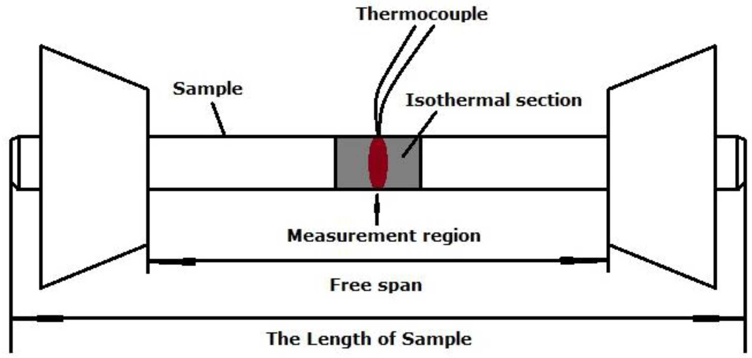
2.4. Material and Dilatometric Testing

The hypo-eutectoid steel, SA508 Gr.3, was investigated with the chemical composition listed Table 1. Figure 1 shows its initial microstructure consisted of pearlite (about 35.8 vol. %) and ferrite determined using quantitative metallography.

Table 1. Chemical composition of SA508 Gr.3 steel.

Element	C	Mn	Si	Ni	Cr	Mo	V	Al	N	Fe
Composition (wt. %)	0.20	1.47	0.17	0.89	0.13	0.51	0.001	0.039	0.014	Bal.

Table 1. Chemical composition of SA508 Gr.3 steel.

Element	C	Mn	Si	Ni	Cr	Mo	V	Al	N	Fe
Composition (wt. %)	0.20	1.47	0.17	0.89	0.13	0.51	0.001	0.039	0.014	Bal.

Figure 1. Initial microstructure of SA508 Gr.3 steel.

Figure 1. Initial microstructure of SA508 Gr.3 steel.

Both the dilatometric tests and validation experiments were carried out on a Gleeble-3500 thermal simulation testing machine, using cylindrical samples with diameter of 6 mm and length of 82 mm. In the dilatometric tests, the variation of diameter is measured. K-Type thermocouples (0.25 mm diameter) are used for the temperature measurements, which are spot-welded on the surface of the middle section of the sample (Figure 2). The sample is heated by resistance heating using low frequency current in the Gleeble system. Due to small skin effect, there is an isothermal section vertical to the length, i.e., the temperature distribution in the central cross section of the sample is homogeneous. The thermocouple measures and controls the temperature of this section, instead of whole specimen, by a closed-loop control system. The continuous thermal dilatometric curves were obtained from 293 K to 1173 K, with 15 different heating rates (β) in a range of 0.008~500 K/s. When the related results are presented in the following sections, only limited representative data are marked in detail, instead of all of them being included, in order to avoid crowding in the figures, etc.

Figure 2. Sketch of dilatation measurement using Gleeble-3500 thermal simulation testing machine.

Figure 2. Sketch of dilatation measurement using Gleeble-3500 thermal simulation testing machine.

In order to demonstrate that the isoconversional method can be used to accurately predict the austenitization during the practical heating processes, a heating process with non-constant heating rates was investigated in this study, and the specific heating process is shown in Figure 3.

Figure 3. A specific continuous heating process with non-constant heating rates designed for SA508 Gr.3 steel.

Figure 3. A specific continuous heating process with non-constant heating rates designed for SA508 Gr.3 steel.

3. Results and Discussion

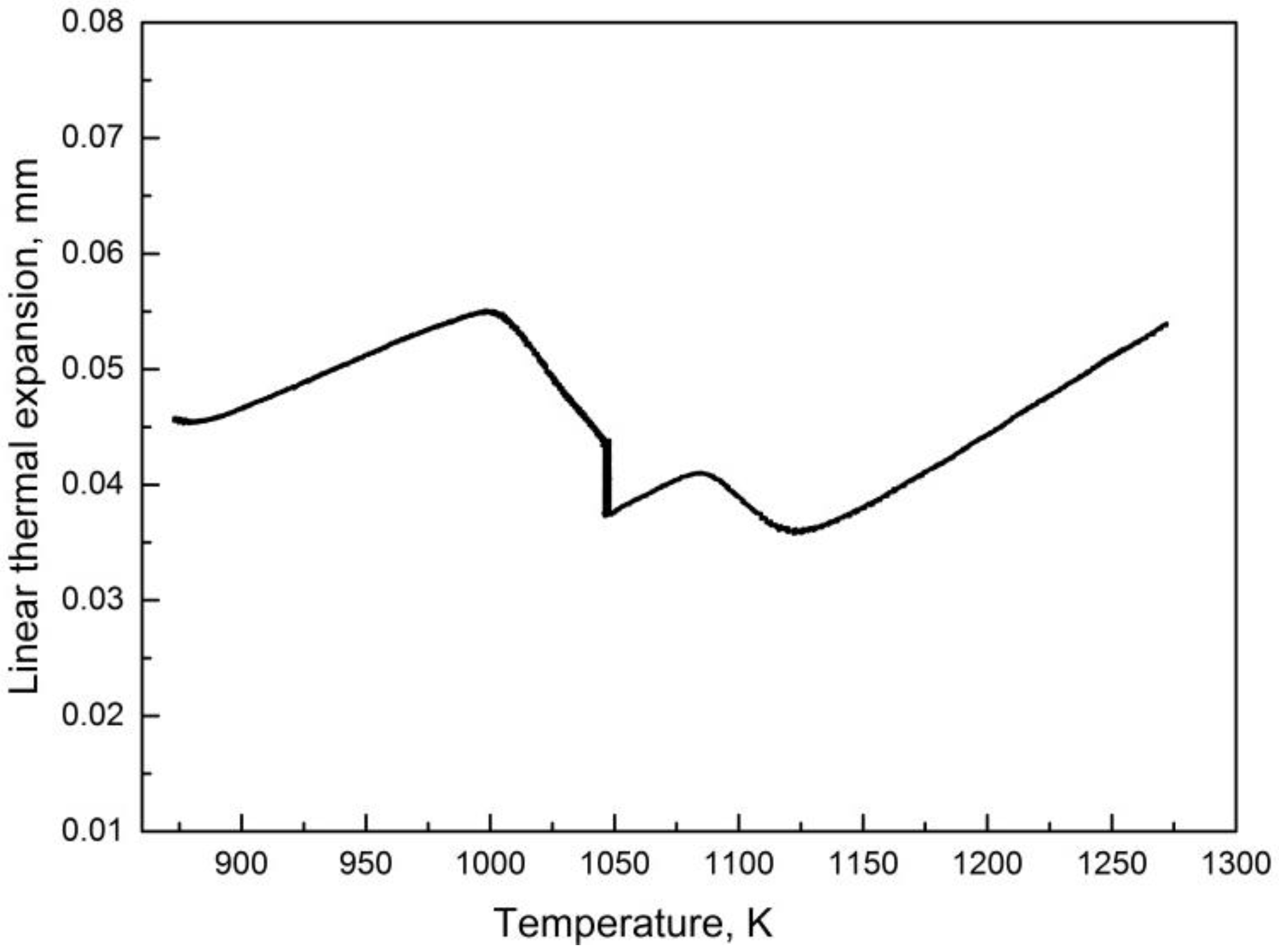
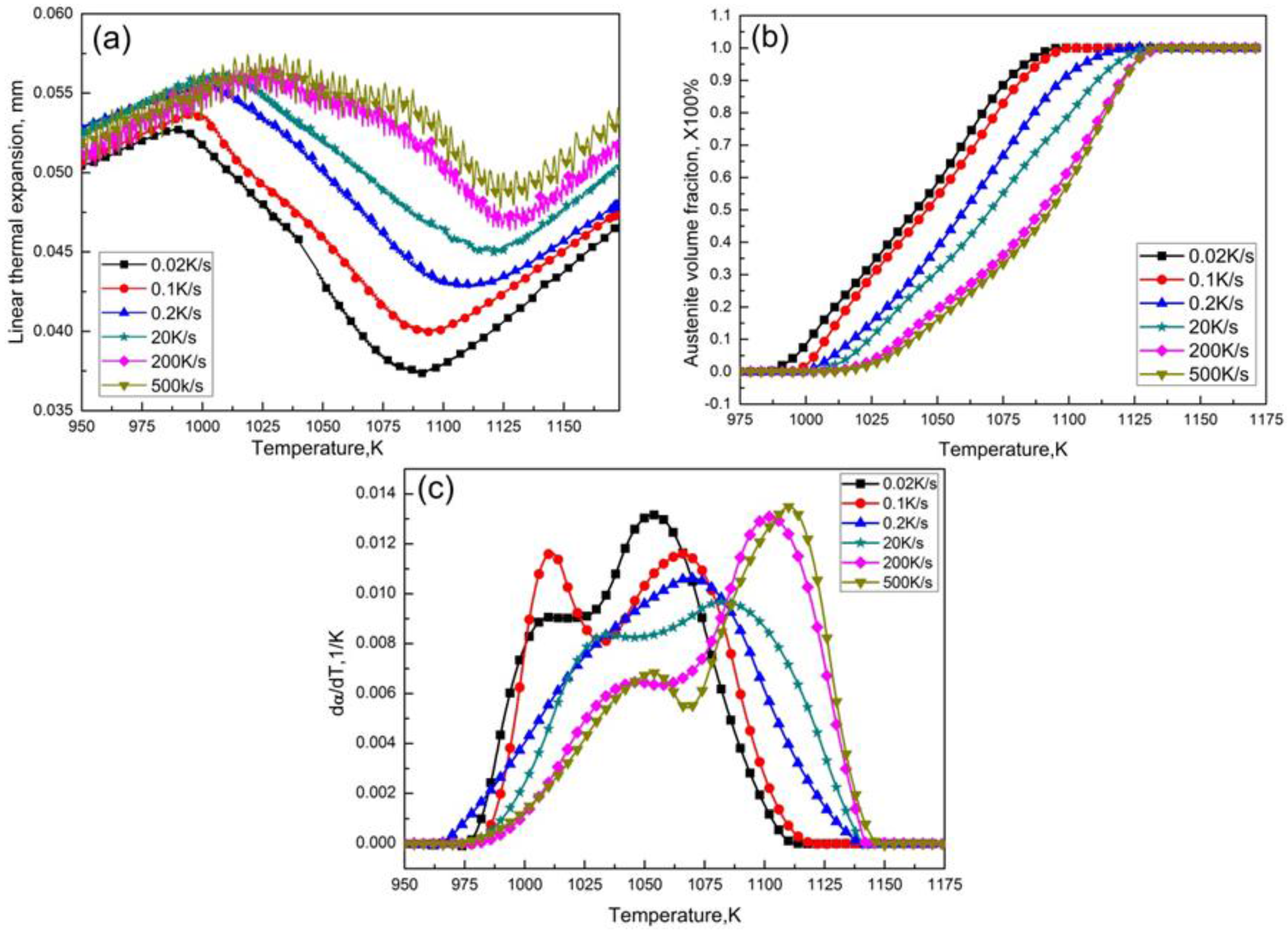
3.1. Data Processing

Figure 4a shows the recorded dilatometric curves with different heating rates (β). The volume fraction (α) of austenite formed during continuous heating was calculated by applying the lever rule, as shown in Figure 4b; Figure 4c is the differential from of the α–T dependence. It is found that most of the dα/dt vs. T curves for different β exhibit two peaks, indicating two maximum phase transformation rates corresponding to the two phase transformation stages, the dissolution of pearlite and ferrite transforming to austenite, respectively, occurred during austenitization. The temperatures of the maximum phase transformation rate increase with β, suggesting that a quicker heating rate results in a delay of the austenitization start temperature.

Figure 4. (a) The measured dilatometric curves; (b) the calculated transformation fraction α; (c) and the dα/dt vs. T curves of SA508 Gr.3 steel at different heating rates, as marked.

Figure 4. (a) The measured dilatometric curves; (b) the calculated transformation fraction α; (c) and the dα/dt vs. T curves of SA508 Gr.3 steel at different heating rates, as marked.

Since the β is constant in individual, continuous heating experiments, the transformation rate can be expressed as:

$$\frac{\text{d}\mathsf{\alpha }}{\text{d}t}=\frac{\text{d}\mathsf{\alpha }}{\text{d}T}\times \mathsf{\beta }$$

(12)

Taking logarithmic of Equation (12) and substituting it into Equation (11), the relationship between ln(dα/dt) and 1/RT(t) is established. The method of determination of E_α(α) and ln(A′(α)) is described as follows: Considering α = 0.5 as an example, the temperatures T reaching α = 0.5 for individually specified β are found in Figure 4b, and the corresponding ln(dα/dt) and 1/RT(t) can be read in Figure 4c. Taking into account all 15 sets of continuous heating experiments, the values of ln(dα/dt) and 1/RT(t) for a fixed α are collected. Based on these data, an Arrhenius plot describing the dependence of ln(dα/dt) on 1/RT(t) can be established using linear fitting (Figure 5). Hence, according to the isoconversional method (Equation (11)), the values of E_α(α) and ln(A′(α)) for α = 0.5 can be determined from the slope and intercept of the fitted line, respectively. In the present study, 25 various α dispersed in a wide range of 0 to 1.0 were considered, and, for a simplified presentation, the Arrhenius plots at selected heating rates α = 0.1, 0.35, 0.5, and 0.7 are shown in Figure 5.

Figure 5. The Arrhenius plots at different heating rates when α = 0.1, 0.35, 0.5, and 0.7.

Figure 5. The Arrhenius plots at different heating rates when α = 0.1, 0.35, 0.5, and 0.7.

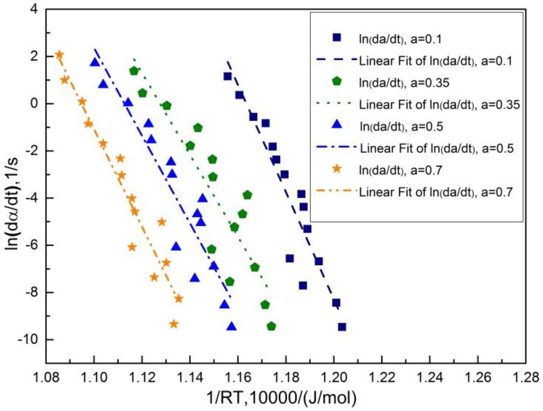
3.2. Determination of Model-Free Austenitization Kinetics

The effective activation energy E_α(α) and modified pre-exponential ln(A′(α)) are the two input parameters necessary for predicting phase transformation kinetics. Based on the isoconversional method, and that of data processing, the dependence of E_α(α) and ln(A′(α)) on α were determined without explicitly assuming a particular form of the transformation model f(α). That is to say, the model-free austenitization kinetics can be determined using this method.

As illustrated in Figure 6, E_α(α) is not a constant value, but changes with the extent of the austenitization process. The curve of E_α(α) vs. α is characterized with a roughly “V” shape. E_α(α) declines with the increasing extent of transformation at the early stage of austenitization (0 ≤ α ≤ 0.35), and then increases until the completion of austenitization. The minimum E_α(α) is at α ≈ 0.35, which is in accord with the initial microstructure composition of the SA508 Gr.3 steel, namely, 35.8 vol. % pearlite and 64.2 vol. % ferrite. The reason for such a V-shaped change trend of E_α(α) is due to the two distinct stages, dissolution of pearlite and transformation of ferrite to austenite, occurring successively in the process of austenitization. As shown in Figure 6, the calculated E_α(α) varies in a range of 1760~2670 kJ/mol during the progress of the austenitization process, similar to, but rather higher, than those reported in the literature (e.g., 2367 kJ/mol [28], 840 kJ/mol and 470 kJ/mol [29]). This can be explained by the differences between the two different forms of the JMAK equation.

Figure 6. The model-free austenitization kinetics determined by the isoconversional method.

Figure 6. The model-free austenitization kinetics determined by the isoconversional method.

As previously mentioned, the kinetics of austenitization in general is mostly described by the JMAK equation. However, there are two commonly used different forms, and the form (I) (Equation (1)) is used in our study. Another form (form (II)) is the original one proposed by Avrami, and is more popular, which can be expressed as follows:

α = 1 – exp[−k(T)tⁿ]

(13)

According to Kohout [1], if the JMAK equation is used in combination with the Arrhenius Equation k(T) = Aexp(−E/RT), the types of equations are not dependent on the choice between JMAK equation forms (I) and (II). The difference consists only in the values of parameters A and E. The application of forms (I) and (II) leads to different values of activation energies: The value E_(II) corresponding to form (II) is equal to the product nE_(I), where the value E_(I) corresponds to form (I). Therefore, the value of effective activation energy of austenitization for SA508 Gr.3 steel, obtained by form (I) in our study, is not comparable to that of the real one using form (II). The real one should be calculated based on form (II). In this case, the real effective activation energy of austenitization for SA508 Gr.3 steel can be obtained from the activation energy using form (I). When “high effective activation energy” (1760~2670 kJ/mol) multiplies n, where the value of n for the whole process of austenitization extracted from our experimental data is about 0.13~0.18 (Figure 7), we can get the real effective activation energy within the range of 229 to 480 kJ/mol. These data are more close to the “commonly referred” effective activation energy value of transformation in steels, and should be reasonably acceptable. The reason for using form (I) in our paper is due to the convenience of data processing in order to acquire the effective activation energy. The effective activation energy, acting as an important parameter in austenization simulation based on the isoconversional method, is extracted from the experiment data.

Figure 7. The parameters n in the JMAK equation for the whole austenitization process of SA508 Gr.3 steel.

Figure 7. The parameters n in the JMAK equation for the whole austenitization process of SA508 Gr.3 steel.

The modified pre-exponential ln(A′(α)) shows a changing trend, similar to that of the effective activation energy, as seen in Figure 6. When the transformation faction is below ~0.35, the ln(A′(α)) decreases with an increasing extent of transformation, and then increases gradually until the completion of austenization completion.

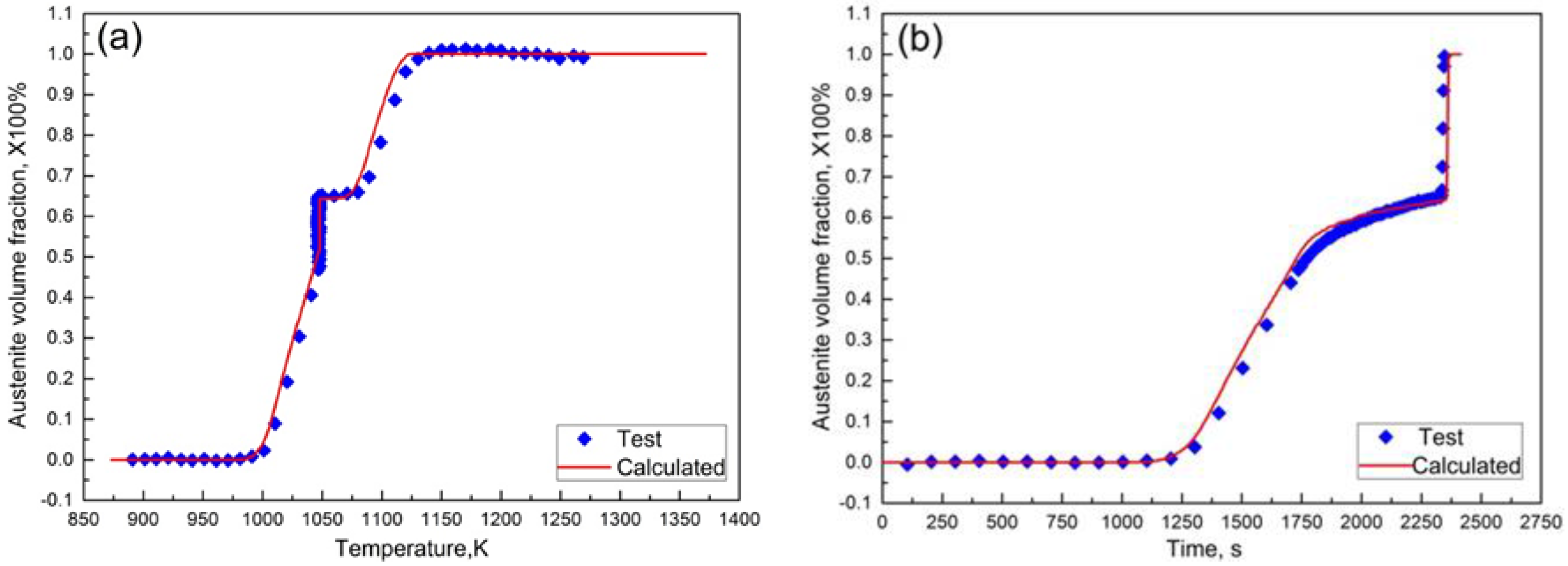
3.3. Regression Validation

The transformation progress can be calculated using the integral form of the isoconversional method, the following equation (Equation (14)), which is:

$${\displaystyle {\int }_0^{\mathsf{\alpha }}\frac{\text{d}\mathsf{\alpha }}{f\left(\mathsf{\alpha }\right)}}=\frac{A(\mathsf{\alpha })}{\mathsf{\beta }}{\displaystyle {\int }_{T_{\mathsf{\alpha }0}}^T\exp \left[-\frac{E_{\mathsf{\alpha }}(\mathsf{\alpha })}{RT}\right]}\text{d}T$$

(14)

For the infinitesimal range of transformation progress Δα, Equation (14) can be rewritten as:

$${\displaystyle {\int }_{\mathsf{\alpha }\to \Delta \mathsf{\alpha }}^{\mathsf{\alpha }}\frac{\text{d}\mathsf{\alpha }}{f\left(\mathsf{\alpha }\right)}}=\frac{A(\mathsf{\alpha })}{\mathsf{\beta }}{\displaystyle {\int }_{T_{\mathsf{\alpha }\to \Delta \mathsf{\alpha }}}^T\exp \left[-\frac{E_{\mathsf{\alpha }}(\mathsf{\alpha })}{RT}\right]}\text{d}T$$

(15)

If Δα is very small, the effective activation energy E_α(α) can be assumed to be constant. Based on the theorem of the average value, for Δα → 0, Equation (15) can be transformed into:

$$\mathsf{\alpha }={\displaystyle \sum _{i=0}^{m}A\prime ({\mathsf{\alpha }}_i)\exp \left[-\frac{E_{\mathsf{\alpha }}({\mathsf{\alpha }}_i)}{R{T}_i}\right]}\Delta t$$

(16)

Using this equation, the transformation progress of austenitization in a specific thermal process can be calculated.

To validate regression the model-free austenitization kinetics (E_α(α)$$and A′(α)) derived from the experimental data, the dependence of transformation fraction α on temperature T was calculated for the thermal programs, identical to the continuous thermal dilatometric experiments. As shown in Figure 8, a good agreement is found to exist between them and, hence, indicates that the isoconversional method allows an accurate determination of the model-free austenitization kinetics.

Figure 8. Comparison between experimental and calculated results of transformation fractions α during continuous heating with various constant heating rates.

Figure 8. Comparison between experimental and calculated results of transformation fractions α during continuous heating with various constant heating rates.

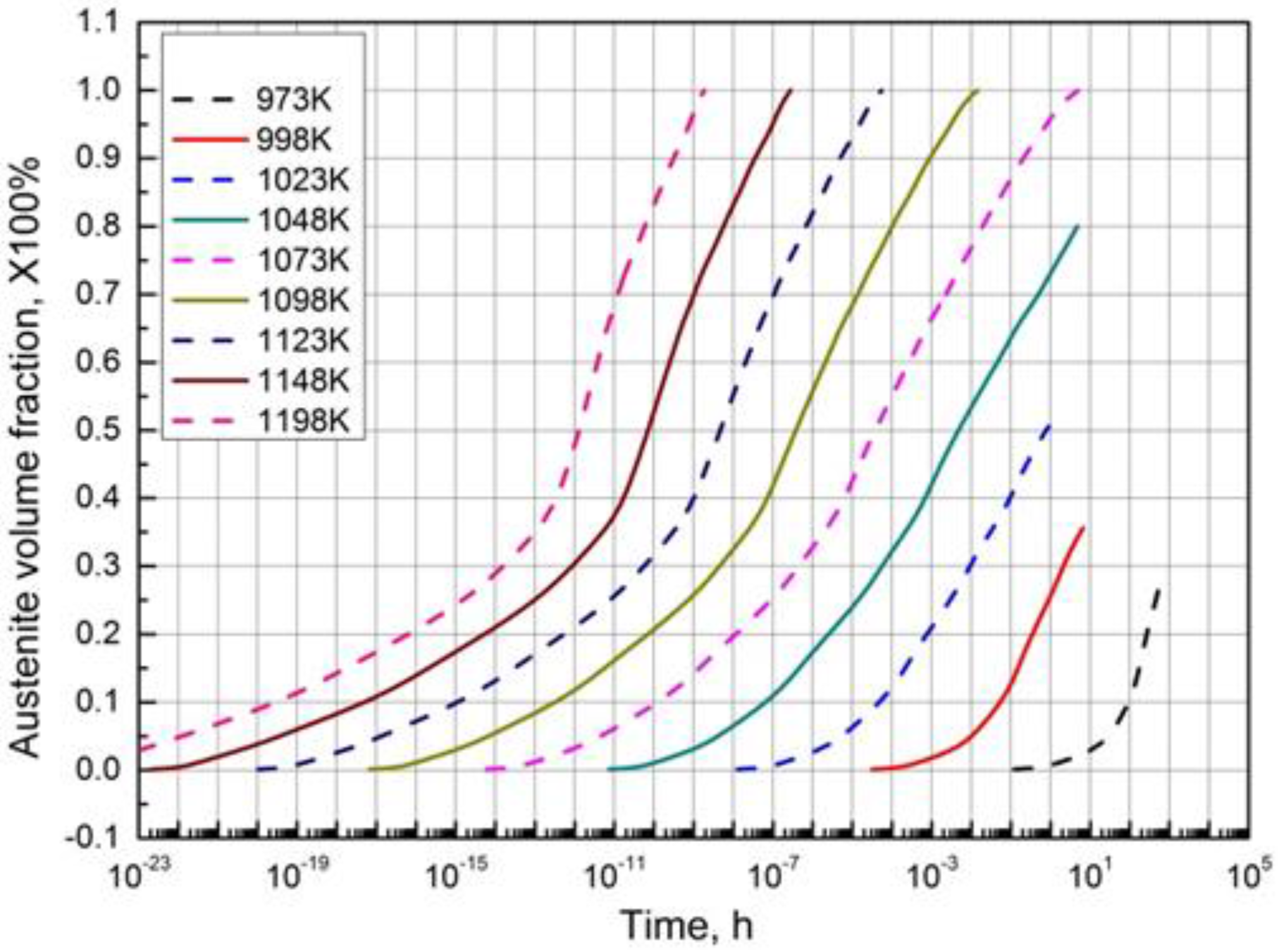
3.4. Calculation of TTA Diagram

Generally, it is difficult to obtain the TTA diagram of steels by experiments. However, it can be conveniently calculated, using the isoconversional method. Taking integration of Equation (10), it yields [30]:

$$t\mathsf{\alpha }={\displaystyle {\int }_0^t\text{d}t}={\displaystyle {\int }_{{\mathsf{\alpha }}_0}^{\mathsf{\alpha }}\frac{\text{d}\mathsf{\alpha }}{A\prime (\mathsf{\alpha })\exp \left[-\frac{E\mathsf{\alpha }(\mathsf{\alpha })}{RT(t)}\right]}}$$

(17)

where t_α is the time to reach a given transformation fraction α. Based on Equation (17), the kinetic predictions for any temperature is possible.

For SA508 Gr.3 steel, when temperature is between the A₁ and A₃, two phases, ferrite and austenite, coexist, and, thus, the maximum transformation fraction of austenitization at a specified temperature has a limit. Considering the influence of alloying elements contained in the present SA508 Gr.3 steel on the Fe–C Phase Diagram, the thermodynamic software JMatPro^® was used to recalculate the Ae₃ line, as seen in Figure 9. Then, based on the calculated Ae₃, using the lever rule, the maximum equilibrium transformation fraction γ_max of the steel was also calculated at a specific temperature, shown as the blue dotted line in Figure 9.

Figure 9. The Ae₃ and maximum austenite transformation fraction γ_max of SA508 Gr.3 steel as the function of temperature T.

Figure 9. The Ae₃ and maximum austenite transformation fraction γ_max of SA508 Gr.3 steel as the function of temperature T.

Finally, taking the influence of the maximum transformation fraction into account, the TTA diagram of SA508 Gr.3 steel (Figure 10) was constructed using the isoconversional method (Equation (17)) and the model-free austenitization kinetics.

Figure 10. TTA diagram of SA508 Gr.3 steel.

Figure 10. TTA diagram of SA508 Gr.3 steel.

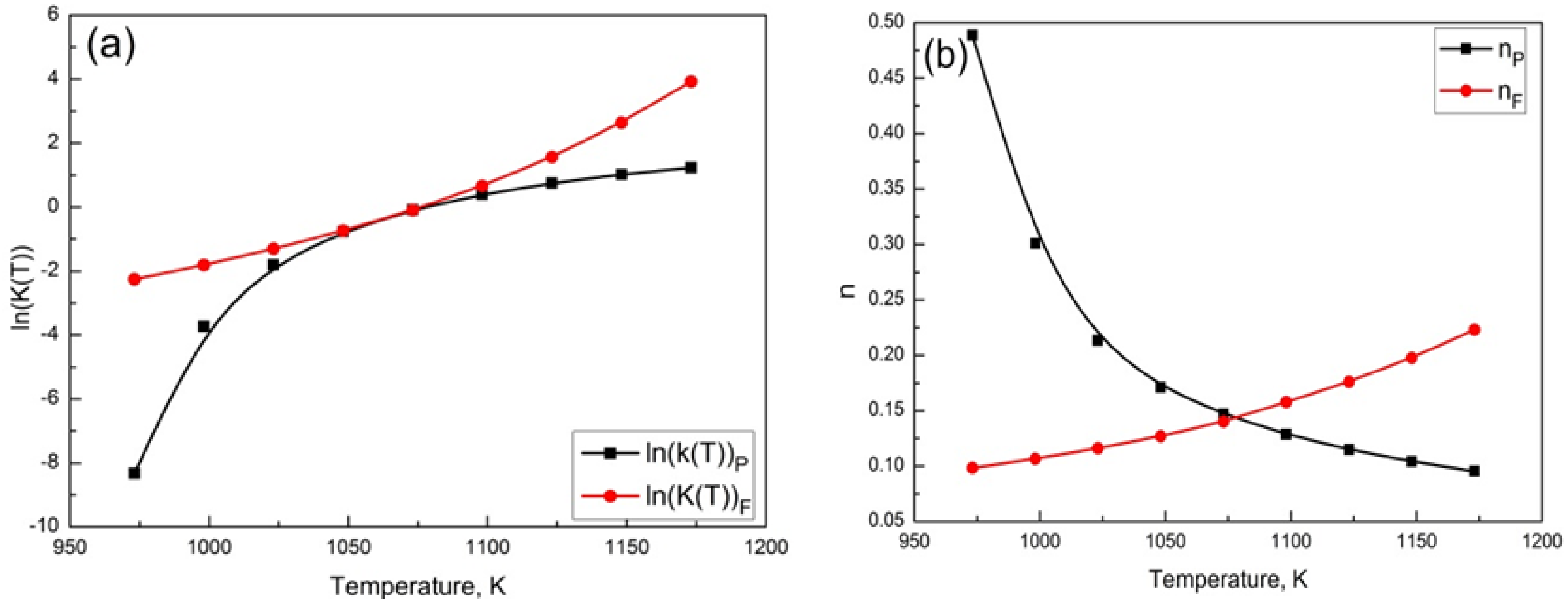
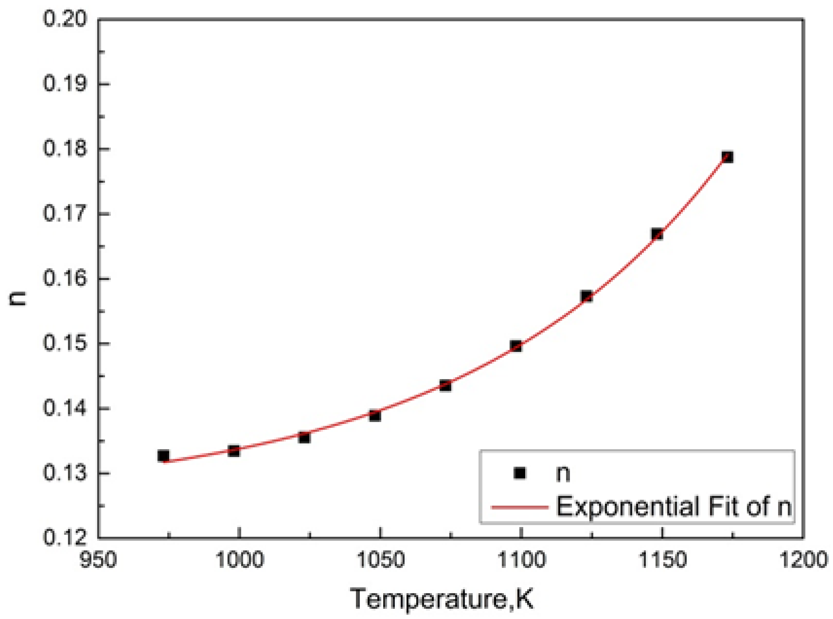
3.5. Determination of the Parameters k(T) and n in JMAK Equation Based on TTA Diagram

The JMAK equation (Equation (1)) gives rise to the transformation fraction α as a function of time t during austenitization. Taking its logarithmic, the equation can be expressed as:

$$\ln \left(\frac{1}{1-\mathsf{\alpha }}\right)=n[\ln \left(k(T)\right)+\ln t]$$

(18)

If using the JMAK equation, the parameters k(T) and n should be given previously. Based on the TTA diagram predicted by the isoconversional method (Equation (17)), the parameters of k(T) and n can be fitted according to Equation (18) and the results are shown in Figure 11, in which the subscripts P and F denote the stages of pearlite dissolution and ferrite to austenite transformation, respectively. It is seen that both the ln(k(T)) for two stages increase with increasing temperature, but compared with ln(k(T))_F, ln(k(T))_P increases faster at lower temperatures, but slower at higher temperatures. For parameter n, n_p decreases with increasing temperature, while n_F exhibits in an opposite way.

Figure 11. The parameters (a) ln(k(T)) and (b) n in JMAK equation as a function of T.

Figure 11. The parameters (a) ln(k(T)) and (b) n in JMAK equation as a function of T.

3.6. Prediction of Austenitization Process during Heating with Non-Constant Heating Rates

In the heating processes considered above, only the ideal thermal conditions (isothermal or constant rate heating) were investigated. However, in real heating processes, such conditions are difficult to be practically performed. It must be very much anticipated to see whether the isoconversional method (Equations (14) and (17)) can also be used to predict the austenitization during the real heating processes accurately or not. Therefore, a specific continuous heating process with non-constant heating rates designed for SA508 Gr.3 steel has been investigated in this work, while the dilatometric curve obtained from the corresponding validation experiment is plotted in Figure 12. Using the isoconversional method, the dependencies of transformation fraction α on temperature T and time t during the heating process, corresponding to that in Figure 3, were predicted. The results are shown in Figure 13, together with those of the experimental measurements, respectively.

Figure 12. The dilatometric curve for SA508 Gr.3 steel during continuous heating with non-constant heating rates, as shown in Figure 3.

Figure 12. The dilatometric curve for SA508 Gr.3 steel during continuous heating with non-constant heating rates, as shown in Figure 3.

Figure 13. Comparison between experimental and predicted curves of transformation fraction α vs. (a) temperature T and (b) time t, respectively, of SA508 Gr.3 steel during continuous heating with non-constant heating rates, as shown in Figure 3.

Figure 13. Comparison between experimental and predicted curves of transformation fraction α vs. (a) temperature T and (b) time t, respectively, of SA508 Gr.3 steel during continuous heating with non-constant heating rates, as shown in Figure 3.

The comparison clearly shows that the predicted and experimental results are in satisfactory agreement and, thus, the isoconversional method allows a reliable and feasible prediction for the austenitization kinetics, even under real heating processes.

4. Conclusions

In this paper, the isoconversional method, incorporating continuous thermal dilatometric tests, has been employed in the study of the austenitization kinetics for SA508 Gr.3 steel during heating. Based on the experimental investigation and numerical calculations, the following conclusions can be drawn:

(1)

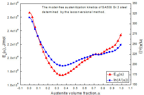
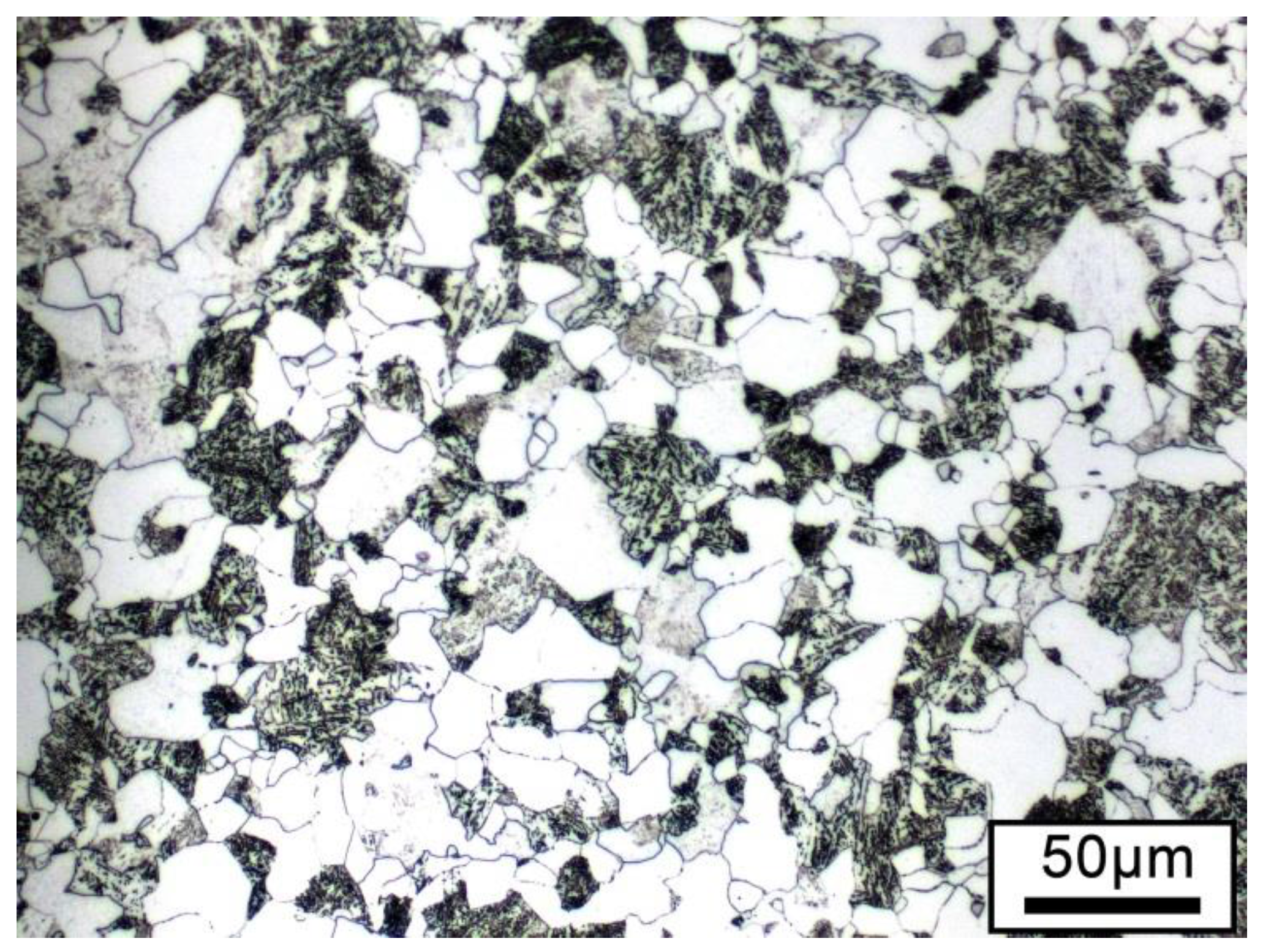
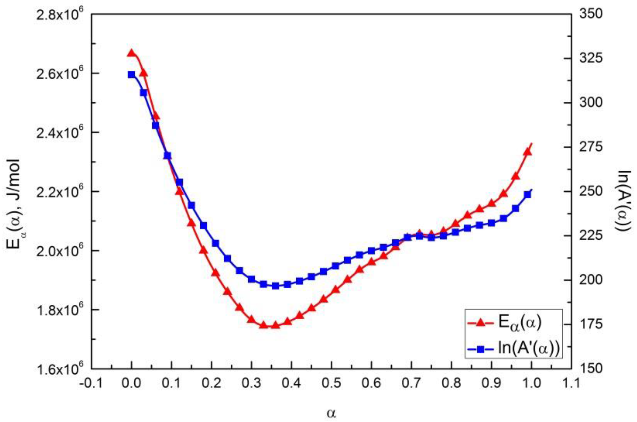
The model-free austenitization kinetics is built by the isoconversional method, and the effective activation energy E_α(α) is also determined. The curve of E_α(α) vs. α is characterized with a roughly “V” shape. The value of E_α(α) is in the range of 1760 to 2670 kJ/mol, and reach a minimum at α ≈ 0.35, consistent with what expected from the initial dual phase (ferrite and pearlite) microstructure of the investigated steel.

(2)

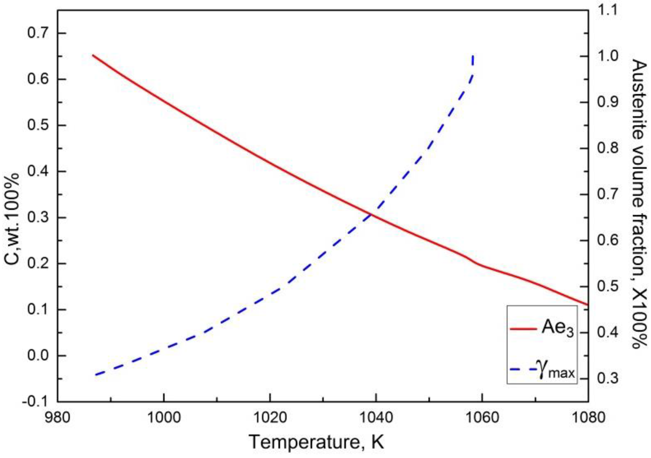
Further, the TTA diagram of SA508 Gr.3 steel has been obtained using the model-free austenitization kinetics and the isoconversional method, providing an effective way for the accurate determination of a TTA diagram, which is usually difficult to obtain from experiments.

(3)

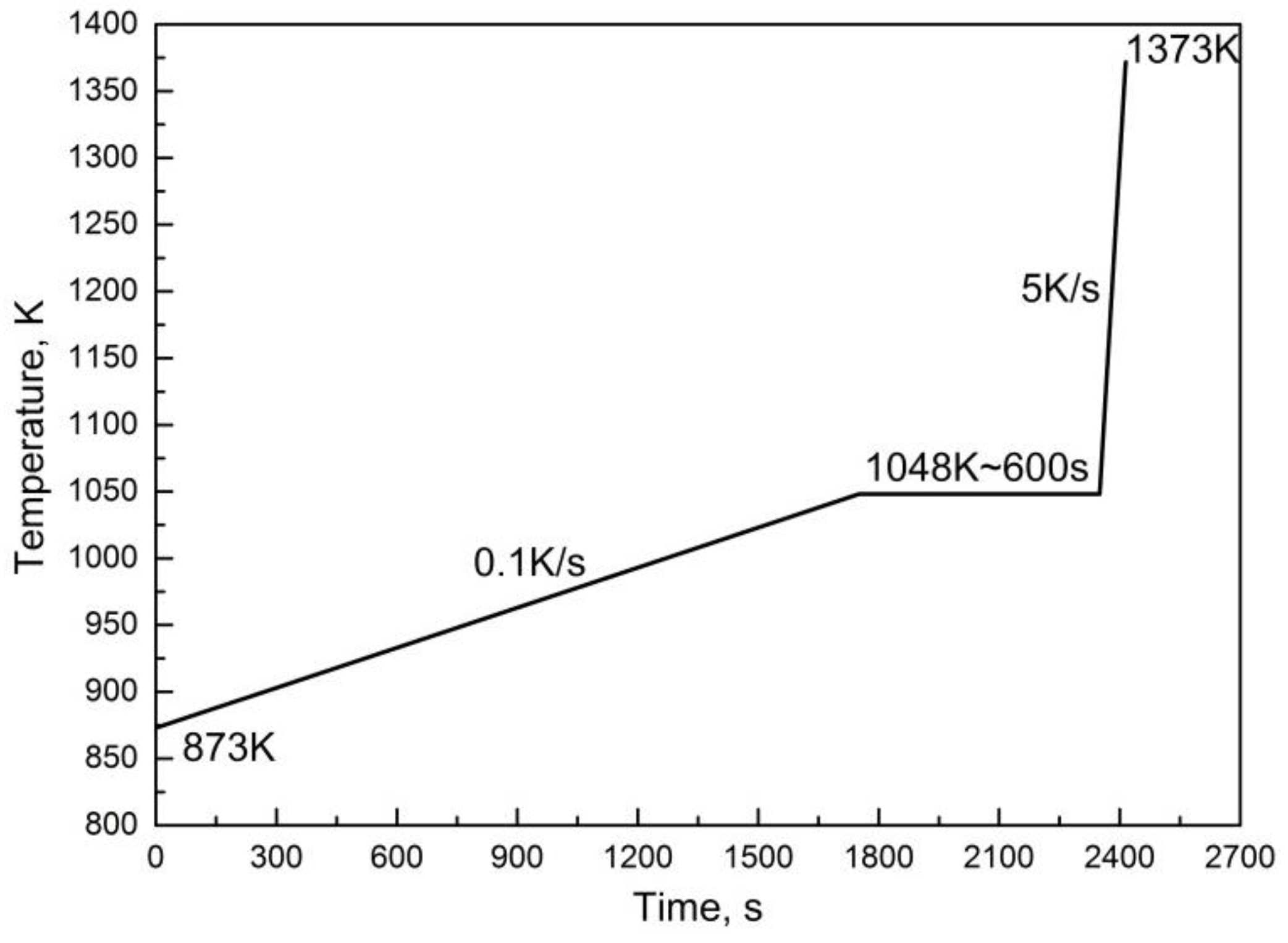
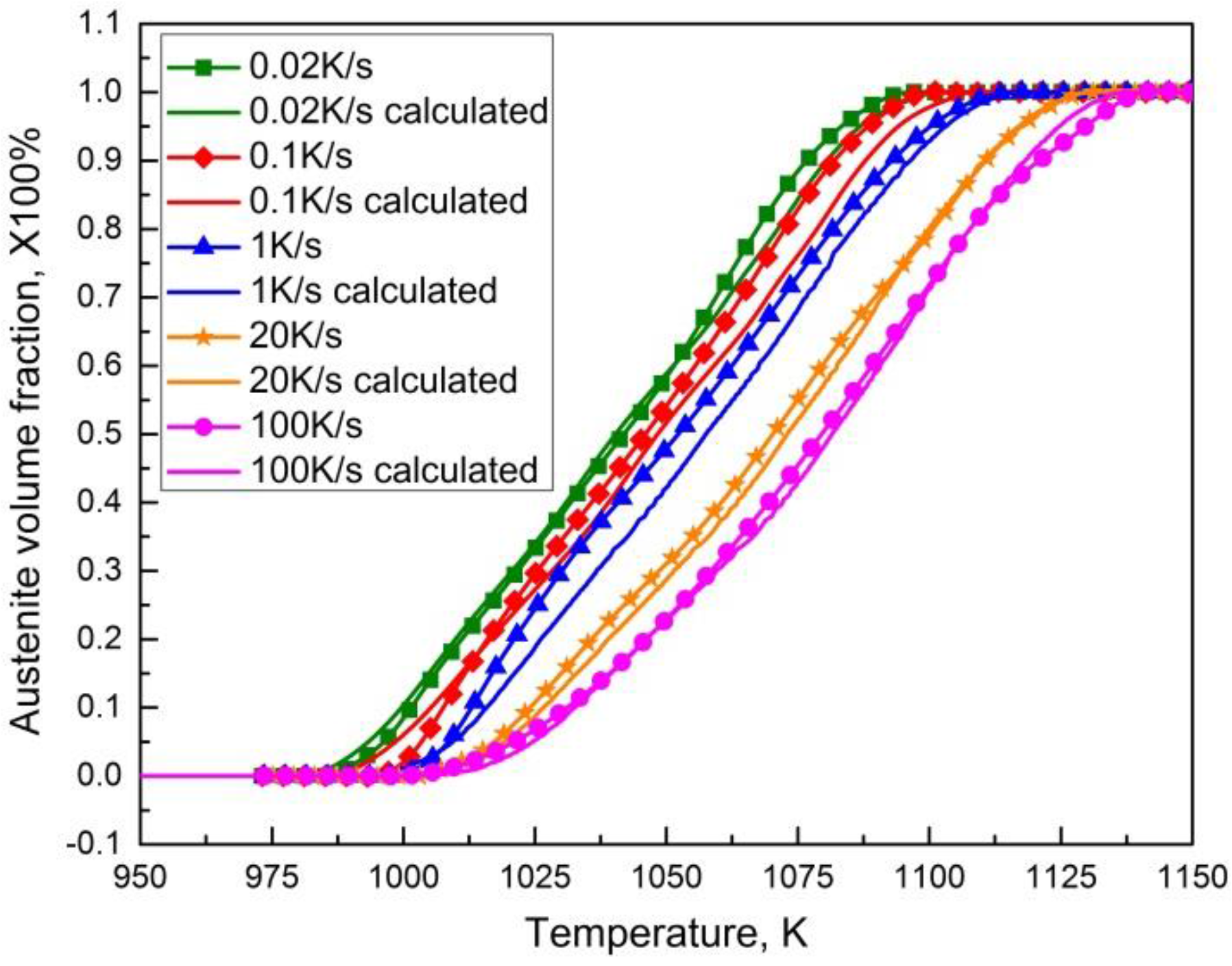
Under non-constant heating rate conditions, a satisfactory agreement between the curve of the phase transformation fraction using numerical prediction with the established model-free austenitization kinetics and that of the calculation from validation dilatometric curve, demonstrates that the isoconversional method can be used to characterize the austenitization kinetics during the heating process.

References

1. Kohout, J. An alternative to the JMAK equation for a better description of phase transformation kinetics. J. Mater. Sci. 2008, 43, 1334–1339. [Google Scholar] [CrossRef]
2. Roosz, A.; Garcia, Z.; Fuchs, E.G. Isothermal formation of austenite in eutectoid plain carbon steel. Acta Mater. 1983, 31, 509–517. [Google Scholar] [CrossRef]
3. De Andrés, C.G.; Caballero, F.G.; Capdevila, C.; Bhadeshia, H.K.D.H. Modelling of kinetics and dilatometric behavior of non-isothermal pearlite-to-austenite transformation in an eutectoid steel. Scr. Mater. 1998, 39, 791–796. [Google Scholar] [CrossRef]
4. Caballero, F.G.; Capdevila, C.; de Andrés, C.G. Kinetics and dilatometric behaviour of non-isothermal ferrite-austenite transformation. Mater. Sci. Technol. 2001, 17, 1114–1118. [Google Scholar] [CrossRef] [Green Version]
5. Caballero, F.G.; Capdevila, C.; de Andrés, C.G. Modelling of kinetics of austenite formation in steels with different initial microstructures. ISIJ Int. 2001, 41, 1093–1102. [Google Scholar] [CrossRef] [Green Version]
6. Gaude-Fugarolas, D.; Bhadeshia, H. A model for austenitisation of hypoeutectoid steels. J. Mater. Sci. 2003, 38, 1195–1201. [Google Scholar] [CrossRef]
7. Surm, H.; Kessler, O.; Hoffmann, F.; Zoch, H.W. Modelling of austenitising with non-constant heating rate in hypereutectoid steels. Int. J. Microstruct. Mater. Prop. 2008, 3, 35–48. [Google Scholar] [CrossRef]
8. Tszeng, T.C.; Shi, G. A global optimization technique to identify overall transformation kinetics using dilatometry data—Applications to austenitization of steels. Mater. Sci. Eng. A 2004, 380, 123–136. [Google Scholar] [CrossRef]
9. Tszeng, T.C.; Shi, G.; Purohit, S. Cementite and carbide dissolution in steels during austenitization at high heating rates. In Proceedings of the Modeling Control and Optimization in Ferrous and Nonferrous Industry Symposium, Chicago, IL, USA, 9–12 November 2003; pp. 379–379.
10. Savran, V.I.; Offerman, S.E.; Sietsma, J. Austenite Nucleation and Growth Observed on the Level of Individual Grains by Three-Dimensional X-Ray Diffraction Microscopy. Metall. Mater. Trans. A 2010, 41, 583–591. [Google Scholar] [CrossRef]
11. Esin, V.A.; Denand, B.; Bihan, L.Q.; Dehmas, M.; Teixeira, J.; Geandier, G.; Denis, S.; Sourmail, T.; Aeby-Gautier, E. In situ synchrotron X-ray diffraction and dilatometric sthdy of austenite formation in a multi-component steel: Influence of initial microstructure and heating rate. Acta Mater. 2014, 80, 118–131. [Google Scholar] [CrossRef]
12. Vyazovkin, S.; Burnham, A.K.; Criado, J.M.; Perez-Maqueda, L.A.; Popescu, C.; Sbirrazzuoli, N. ICTAC Kinetics Committee recommendations for performing kinetic computations on thermal analysis data. Thermochim. Acta 2011, 520, 1–19. [Google Scholar] [CrossRef]
13. Flynn, J.H.; Wall, L.A. General Treatment of the Thermogravimetry of Polymers. J. Res. Natl. Bur. Stand. 1966, 70, 487–523. [Google Scholar] [CrossRef]
14. Ozawa, T. A new method of quantitative differential thermal analysis. Bull. Chem. Soc. Jpn. 1966, 39, 2071–2085. [Google Scholar] [CrossRef]
15. Kissinger, H.E. Reaction Kinetics in Differential Thermal Analysis. Anal. Chem. 1957, 29, 1702–1706. [Google Scholar] [CrossRef]
16. Sunose, T.; Akahira, T. Method of determining activation deterioration constant of electrical insulating materials. Res. Rep. Chiba Inst. Technol. 1971, 16, 22–31. [Google Scholar]
17. Vyazovkin, S.; Dollimore, D. Linear and Nonlinear Procedures in Isoconversional Computations of the Activation Energy of Nonisothermal Reactions in Solids. J. Chem. Inf. Comput. Sci. 1996, 36, 42–45. [Google Scholar] [CrossRef]
18. Friedman, H.L. New methods for evaluating kinetic parameters from thermal analysis data. J. Polym. Sci. B Polym. Lett. 1969, 7, 41–46. [Google Scholar] [CrossRef]
19. Friedman, H.L. Kinetics of thermal degradation of char-forming plastics from thermogravimetry. Application to a phenolic plastic. J. Polym. Sci. C Polym. Symp. 1964, 6, 183–195. [Google Scholar] [CrossRef]
20. Luiggi, N.; Betancourt, M. On the non-isothermal precipitation of the β′ and β phases in Al-12.6 mass% Mg alloys using dilatometric techniques. J. Therm. Anal. Calorim. 2003, 74, 883–894. [Google Scholar] [CrossRef]
21. Adorno, A.T.; Carvalho, T.M.; Magdalena, A.G.; dos Santos, C.M.A.; Silva, R.A.G. Activation energy for the reverse eutectoid reaction in hypo-eutectoid Cu–Al alloys. Thermochim. Acta 2012, 531, 35–41. [Google Scholar] [CrossRef]
22. Silva, R.A.G.; Gama, S.; Paganotti, A.; Adorno, A.T.; Carvalho, T.M.; Santos, C.M.A. Effect of Ag addition on phase transitions of the Cu-22.26 at. %Al-9.93 at. %Mn alloy. Thermochim. Acta 2013, 554, 71–75. [Google Scholar] [CrossRef]
23. Vyazovkin, S. Computational aspects of kinetic analysis. Part C. The ICTAC Kinetics Project—The light at the end of the tunnel? Thermochim. Acta 2000, 355, 155–163. [Google Scholar] [CrossRef]
24. Brown, M.E.; Dollimore, D.; Galwey, A.K. Reactions in the Solid State, Comprehensive Chemical Kinetics; Elsevier: Amsterdam, The Netherlands, 1980. [Google Scholar]
25. Brown, M.E. Introduction to Thermal Analysis: Techniques and Applications; Springer Science & Business Media: Lodon, UK, 2001; p. 264. [Google Scholar]
26. Brown, M.E.; Maciejewski, M.; Vyazovkin, S.; Nomen, R.; Sempere, J.; Burnham, A.; Opfermann, J.; Strey, R.; Anderson, H.L.; Kemmler, A.; et al. Computational aspects of kinetic analysis Part A: The ICTAC kinetics project-data, methods and results. Thermochim. Acta 2000, 355, 125–143. [Google Scholar] [CrossRef]
27. Marcilla, A.; Garcia-Quesada, J.C.; Ruiz-Femenia, R. Additional considerations to the paper entitled: “Computational aspects of kinetic analysis. Part B: The ICTAC Kinetics Project—The decomposition kinetics of calcium carbonate revisited, or some tips on survival in the kinetic minefield”. Thermochim. Acta 2006, 445, 92–96. [Google Scholar] [CrossRef]
28. Chen, R.; Gu, J.; Han, L.; Pan, J. Austenization kinetics of 30Cr2Ni4MoV steel. Trans. Mater. Heat Treat. 2013, 34, 170–174. [Google Scholar]
29. Chiba, A. Isothermal transformation kinetics from ferrite to austenite in an Fe-8% Cr alloy. Trans. Jpn. Inst. Met. 1984, 25, 523–530. [Google Scholar] [CrossRef]
30. Burnham, A.K.; Dinh, L.N. A comparison of isoconversional and model-fitting approaches to kinetic parameter estimation and application predictions. J. Therm. Anal. Calorim. 2007, 89, 479–490. [Google Scholar] [CrossRef]