Study of the Tensile Damage of High-Strength Aluminum Alloy by Acoustic Emission

Abstract

The key material of high-speed train gearbox shells is high-strength aluminum alloy. Material damage is inevitable in the process of servicing. It is of great importance to study material damage for in-service gearboxes of high-speed train. Structural health monitoring methods have been widely used to study material damage in recent years. This study focuses on the application of an acoustic emission (AE) method to quantify tensile damage evolution of high-strength aluminum alloy. First, a characteristic parameter was developed to connect AE signals with tensile damage. Second, a tensile damage quantification model was presented based on the relationship between AE counts and tensile behavior to study elastic deformation of tensile damage. Then tensile tests with AE monitoring were employed to collect AE signals and tensile damage data of nine samples. The experimental data were used to quantify tensile damage of high-strength aluminum alloy A356 to demonstrate the effectiveness of the proposed method.

1. Introduction

The gearbox is one of the important parts of a high-speed train, which is subjected to damage in its service life. For example, the gearbox bracket area suffers static and dynamic loads during service. The static load is mainly caused by the weight and load of the train, while the dynamic load is related to a lot of factors including the natural wind, shock and vibration generated by operation of the train, the centrifugal force generated by curve movement of the train and so on. Static and dynamic loads bring both tensile damage and fatigue damage to gearbox bracket. Thus, it is of great importance to ensure the service safety of the gearbox. In this paper, high-strength aluminum alloy A356 is the key material of high-speed train gearbox shells. The performance analysis of the service process for this material has not yet been done [1,2]. It is necessary to develop a structural health monitoring method to study the tensile performance of this material.

In recent years, many studies have focused on developing methods to study in-service material performance by structural health monitoring techniques. Acoustic emission (AE), one of the efficient structural health monitoring techniques, which is defined as a phenomenon of rapid release of energy and generation of transient elastic wave from a localized source of the material [3]. Most of the material damage is related to microscopic processes involving some stress relaxation. Monitoring AE signals from a damaging material can give significant information about the microscopic mechanisms involved, because the magnitude of this stress relaxation is dependent upon the particular process [4].

The AE technique is widely used to detect the occurrence and growth of damage and quantify damage of in-service materials and is not limited by the materials. It has been identified that AE monitoring is capable of detecting material damage over the past three decades [5,6,7]. Previous studies have also proved that AE technique is sensitive and reliable in the detection of material damage for in-service structures [8,9]. The key of studying material tensile damage by using the AE technique is to relate AE parameters to tensile processes. Several attempts have been made to find the relationship between AE parameters and material damage during tensile processes. Haneef et al. [4] studied the tensile behavior of AISI type 316 stainless steel using AE and infrared thermography techniques. They discovered that AE root mean square voltage increased with an increase in strain rate due to the increase in source activation. The dominant frequency of the AE signals generated during different regions of tensile deformation has also been used to compare the results for different strain rates. They found that the dominant frequency of AE signals increased from elastic region to around 580–590 kHz during work hardening and 710–730 kHz around ultimate tensile strength for different strain rates, but they did not give an exact model to quantify tensile damage of the material. Lugo et al. [10] used AE to quantify the microstructural damage evolution under tensile loading for a 7075 aluminum alloy. They proved that the AE activity is related directly with damage progression in this alloy by building a model correlating AE counts to number density, but they focused on capturing ductile material failure. The difference between the elastic stage and plastic stage of tensile processes was ignored. Patrik et al. [11] monitored and analyzed the AE signal during tensile tests of pure Mg and Mg alloys of the AZ series in order to study the influence of alloy composition on plastic deformation. The Kaiser effect was used to determine the stability of the microstructure. They found the post-relaxation effect was sensitive to alloy composition and the strain at which the stress relaxation was performed, but they aimed to study the deformation mechanisms of plastic stage. The deformation mechanisms of the elastic stage were ignored. Godin et al. [12] used the AE technique to discriminate between the different types of damage occurring in a constrained composite. Two main types of signals were identified, originating from the two expected damage mechanisms i.e., matrix cracking and decohesion. They used the k-means algorithm to split the AE data into two classes by counts, duration, and average frequency. Then k-nearest neighbors (KNN) method was used to classify the AE data. However, in their paper, AE signals were from composite materials, the AE signal of aluminum alloys is different. Cousland et al. [13] recorded AE signals during the unidirectional tensile deformation of aluminum alloys 2024 and 2124 to identify the sources of the emission. They concluded that the fracture of brittle inclusions in the primary source of the AE detected during the tensile testing of the alloys in the temper condition T351, but their main work was to find the source of AE signals during tensile fracture. They did not pay attention to quantify elastic deformation. Wen and Morris [14] investigated the effect of different thermal treatment temperatures (from 472 to 783 K) on the characteristics of serrated yielding of three commercial aluminum alloys, AA5052, AA5754, and AA5182 by using the AE technique. They discovered that the acoustic emission appears to be related to the number of Mg atoms actually participating in the dynamic strain aging process, but they concentrate on the yield stage of tensile process.

The AE technique is mainly applied to study plastic deformation during tensile processes. Bohlen et al. [15] observed and analyzed AE signals during plastic deformation of an AZ31 sheet in an H24 original condition, as well as after a heat treatment at elevated temperature. The AE count rates show a well-known correlation with the stress-strain curves. Máthis et al. [16] investigated mechanisms of plastic deformation of a commercial AM60 magnesium alloy by using AE measurements, TEM, and light microscopy. They found that the deformation behavior of the AM60 alloy exhibits three significant stages. Cakir et al. [17] measured the AE response of an implant-quality 205L stainless steel during slow strain rate tensile testing at a constant strain rate of 7.35 × 10⁻⁶. They believed the attenuation of the AE activity beyond necking is attributed to the localization of plastic deformation. Vinogradov et al. [18] performed AE measurements during room temperature tensile deformation of high-alloyed cast model steels with different austenite stability to get a better understanding of the kinetics of TRIP/TWIP-assisted plastic deformation. They identified four different microstructure-related major mechanisms of plastic deformation as AE sources. Kocich et al. [19] discovered the special character of AE signal during plastic deformation, which can be called white noise with low energy. They used UFG materials to identify the limit of detectability. Therefore, the AE technique is available and effective for studying tensile deformation and quantifying tensile damage of materials. Presently, articles focused on quantifying elastic deformation during tensile process by the AE technique are relatively few. There is a need to develop an AE method to quantify elastic deformation of tensile damage.

In this paper, a method of tensile damage quantification by the AE technique was presented. The proposed method was based on the relationship between AE counts and tensile damage. This research focused on quantifying the elastic deformation of tensile damage. The method presented in this paper was a prognostic method only if data obtained from tensile tests was applied. The application of the developed method in high-strength aluminum alloy A356 of high-speed train gearbox shells was given to demonstrate the effectiveness of the proposed method.

The paper is organized as follows. Experimental procedures are described in Section 2. Section 3 then introduces the theoretical method for tensile damage quantification. The application of the proposed method is also introduced in this section. Conclusions will be discussed and summarized in the last section.

2. Experimental Procedures

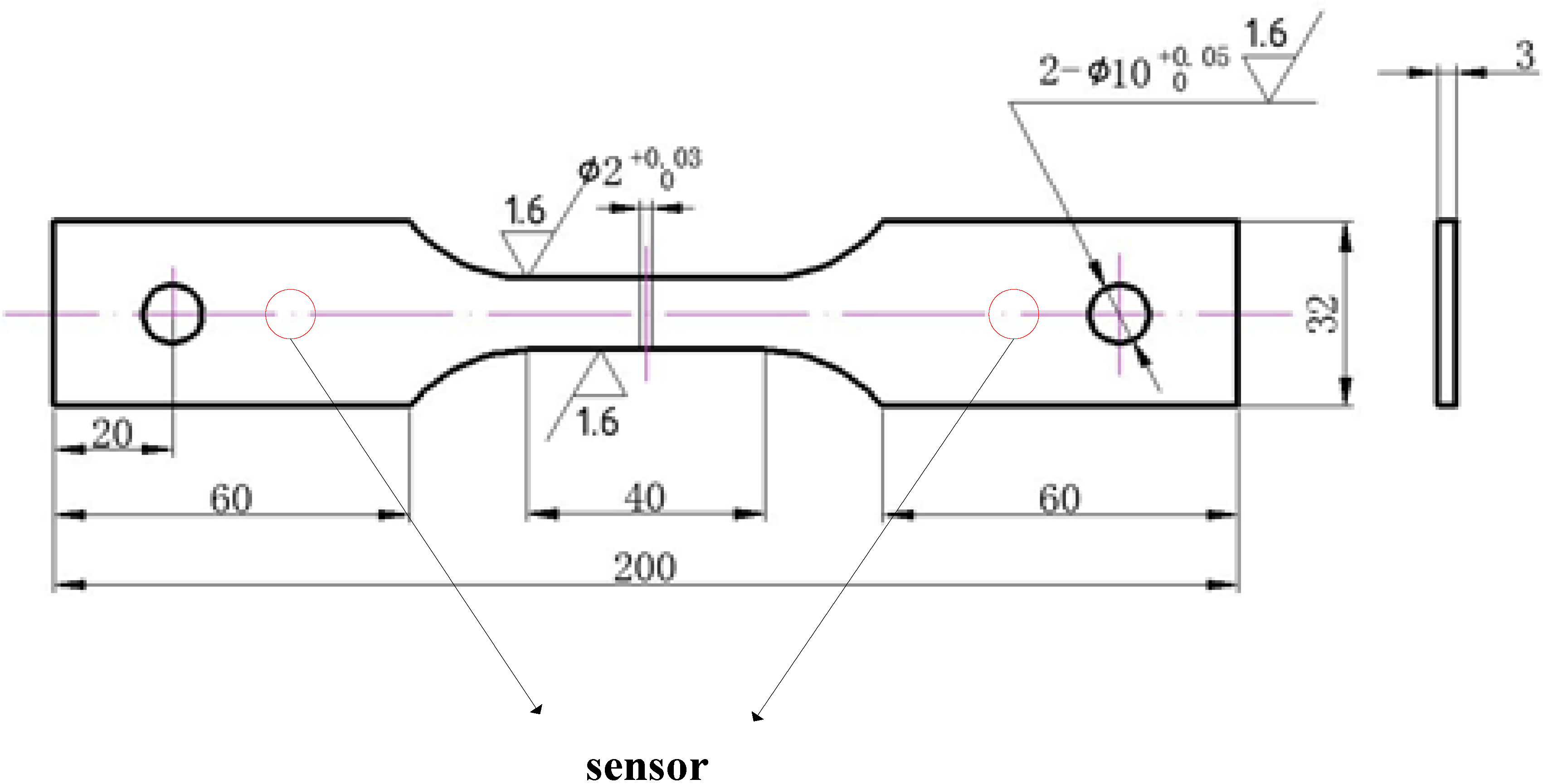
An AE instrument was used to detect and record AE signals during tensile tests. Tensile tests with AE monitoring contained two parts of data, which are tensile damage data and AE monitoring data. The purpose of this study is to analyze the relationship between tensile damage and AE signals to quantify tensile damage of the high-strength aluminum alloy A356 by using AE signals.

2.1. Tensile Test

The material used in this study is high-strength aluminum alloy A356, which has reached excellent properties of rigidity, strength, ductility, fatigue, casting, and shrinkage tendency [20]. Its nominal chemical composition is presented in Table 1.

Table 1. Chemical compositions (wt. %) of the improved aluminum alloy type A356.

Composition	Si	Mg	Ti	Sr
wt. %	6.5~7.5	0.20~0.35	0.08~0.2	0.005~0.015

Table 1. Chemical compositions (wt. %) of the improved aluminum alloy type A356.

Composition	Si	Mg	Ti	Sr
wt. %	6.5~7.5	0.20~0.35	0.08~0.2	0.005~0.015

An 810 Material Test System (MTS) was used to carry out tensile tests. The strain rate was 10⁻⁴/s, and test environment was 27 °C and 40% RH. There are a total of nine tensile samples, which were numbered S1 to S9. Figure 1 shows the geometry of the sample [21]. During the test, increased longitudinal tensile force was applied to the sample. Samples were broken in the end.

Figure 1. Geometry of tensile sample and arrangement of AE sensors, dimensions in mm [21].

Figure 1. Geometry of tensile sample and arrangement of AE sensors, dimensions in mm [21].

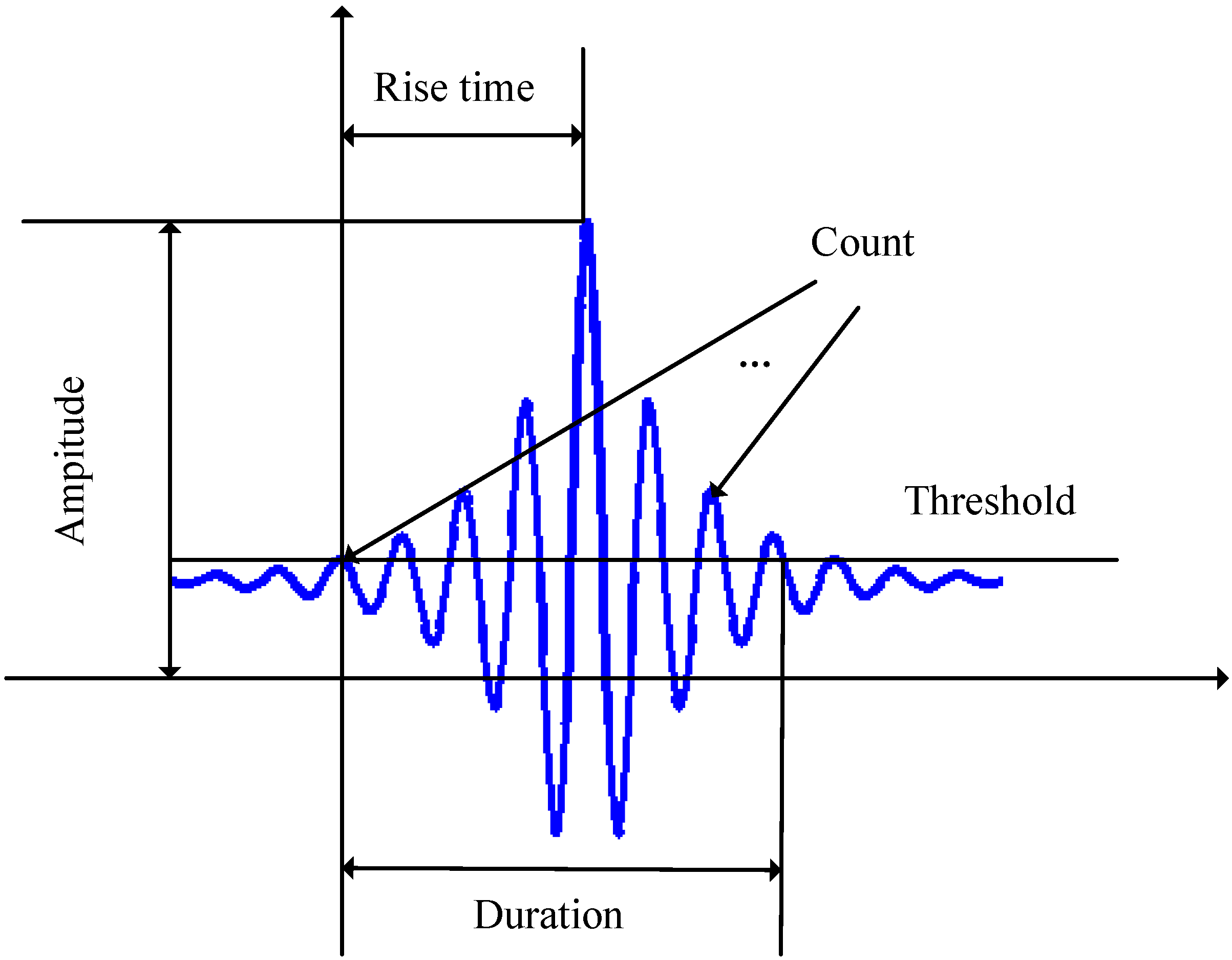
2.2. Acoustic Emission Technology

AE is defined as “a phenomenon of rapid release of energy and generation of transient elastic wave from a localized source of the material” [3]. AE signals are generated from the sudden release of strain energy at the damage sources, which are plastic deformation, crack propagation, wear, friction, and so on [12,22]. AE registration is an effective methodology, which allows “hearing” and registering damage during loading of samples [12].

An AE instrument PCI-2 supplied by American PCA company was performed to record and process AE signals during tensile tests. AE signals were recorded from tensile tests. During elastic deformation of tensile process the AE signals are mainly of continuous type signals. Typical parameters of AE signal are count, energy, amplitude, duration, rise time, and so on. The most commonly used AE parameter is count, which is defined as the number of times that the AE signal amplitude exceeds a predefined subjective threshold value [23]. Figure 2 shows some typical parameters in a burst-type waveform of AE signal.

Figure 2. Typical parameters of AE signal.

Figure 2. Typical parameters of AE signal.

The sensor used in tensile test was standard resonant sensor of type R15A, a 40dB pre-amplification was employed to amplify signals. For all the nine samples Vaseline was used to mount the sensor to the sample surface to ensure the extreme sensitivity of the sensor. Figure 1 shows the arrangement of sensors. Threshold values were set to remove noise, the fixed threshold (trigger level) value was 45 dB in all tests; the energy threshold value was 1. The sampling frequency is 1 MHz; peak identification time (PDT) was 300 μs; impact identification time (HDT) was 600 μs; hit lockout time (HLT) was 1000 μs; and the crash file length was 2kB.

3. Results and Discussion

In this section, a characteristic parameter was developed to connect AE signals with tensile processes. Then, a tensile damage quantification model was presented based on the relationship between AE counts and tensile behavior to quantify tensile damage evolution of high-strength aluminum alloy A356. This paper focused on quantifying the elastic deformation of tensile damage.

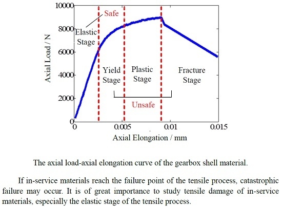
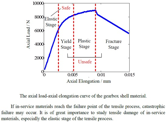
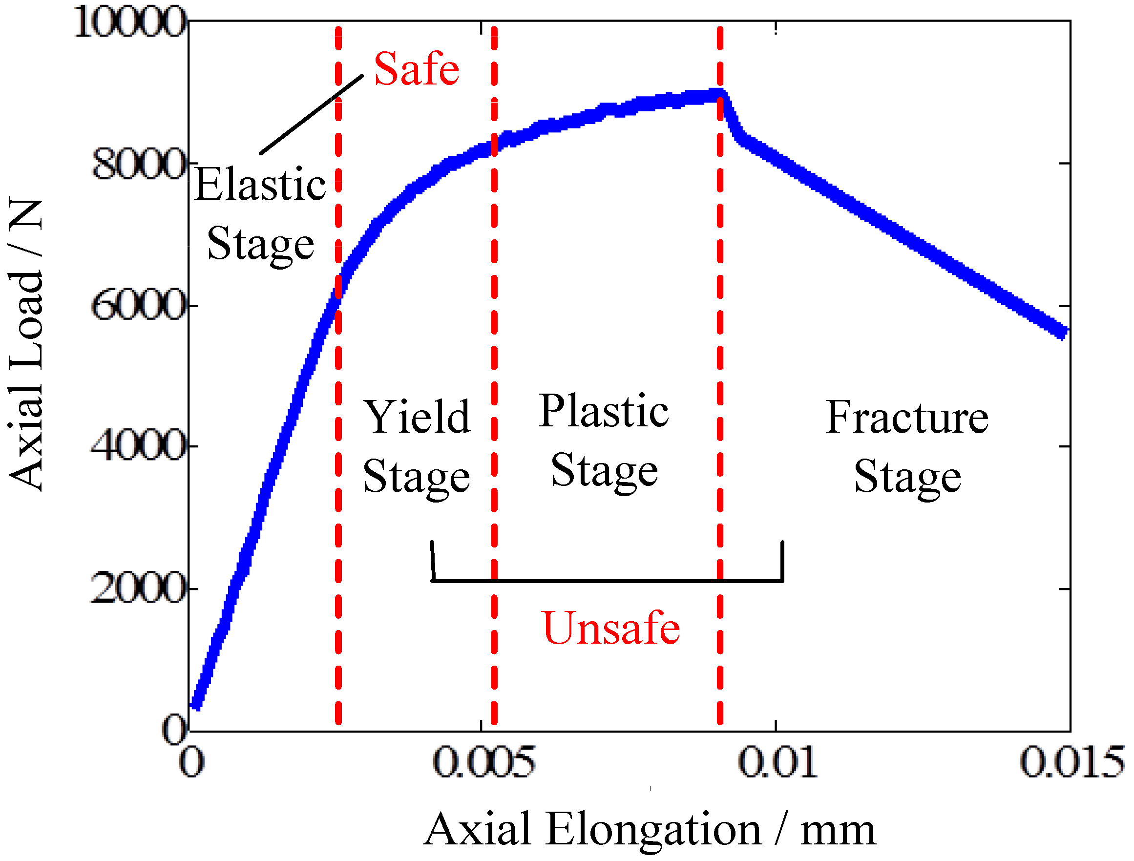
3.1. Material Tensile Damage

The tensile process of metal can be divided into four stages; elastic stage, yield stage, plastic stage, and fracture stage [20]. Figure 3 displays the four stages of tensile process identified on the axial load-axial elongation curve. The four stages can be divided according to different characteristics. At the elastic stage, the material deformation is elastic, the force and elongation is proportional. The elongation will disappear with the force gone, and no residual elongation will occur. When the in-service material is in the elastic stage, it can be considered safe [21], but when the material comes into the yield stage, unrecoverable deformation will be produced. The reliability of the material will be reduced, and the final fracture will come quickly. Thus, the in-service material can be considered unsafe. In this paper, the transition point from elastic stage to yield stage is the failure point of the tensile process [21].

Figure 3. The axial load-axial elongation curve of the gearbox shell material.

Figure 3. The axial load-axial elongation curve of the gearbox shell material.

If in-service materials reach the failure point of the tensile process, catastrophic failure may occur. It is of great importance to study tensile damage of in-service materials, especially the elastic stage of the tensile process. This paper aims to quantify the elastic deformation of material by the AE technique.

3.2. Characteristic of AE Signal for the Tensile Damage

Figure 4 displays the relationship between AE counts and axial elongation in the same tensile process. It is indicated that AE counts increased significantly at the transition point from elastic stage to yield stage [21]. AE counts can be used to characterize the tensile damage, but the AE counts of each sample at the transition point are different, and the values have a great range. Thus, it is necessary to develop a characteristic parameter involving AE counts to find the transition point between the elastic stage and yield stage of the tensile process. The characteristic parameter is the key to relate tensile damage with AE signals.

Figure 4. AE counts and axial elongation curve.

Figure 4. AE counts and axial elongation curve.

In this paper, the characteristic parameter is named AC(t). It can be calculated by Equations (1) and (2):

$$M_j(t)={\text{median}}_m(\frac{t_{j+1}-t_j}{c_j}+\frac{t_{j+2}-t_{j+1}}{c_{j+1}}\cdot \cdot \cdot \frac{t_{j+m}-t_{j+m-1}}{c_{j+m-1}})\begin{array}{cc}& \end{array}j=1,2,\cdot \cdot \cdot ,n$$

(1)

$$A{C}_j(t)=M_{j+1}(t)-M_j(t)$$

(2)

where c_j is the AE count at t_j time; m is the quantity of values used to calculate the median of them; j is the AE count number. Once the value of AC(t) comes into the preset threshold interval, it means that the tensile process reaches the transition point from elastic stage to yield stage. In other words, the duration of the elastic stage t_f can be obtained.

AE signals were collected and recorded from tensile tests with the AE instrument. The characteristic parameter AC(t) was calculated based on Equations (1) and (2). Herein, m = 10 and the threshold interval was [7.65 × 10⁻³, 7.85 × 10⁻³], Once the value of AC(t) reached the preset threshold interval, the duration of the elastic stage t_f can be obtained. Table 2 shows the characteristic parameter AC_f(t) at the transition point and duration of the elastic stage t_f of all nine samples.

Table 2. The results of characteristic parameter AC(t) and duration of the elastic stage t_f.

Sample	tf/s	ACf(t)
S1	88.6	0.000780
S2	73.0	0.000769
S3	88.9	0.000779
S4	95.8	0.000782
S5	122.0	0.000773
S6	129.0	0.000781
S7	111.8	0.000777
S8	159.0	0.000775
S9	92.6	0.000776

Table 2. The results of characteristic parameter AC(t) and duration of the elastic stage t_f.

Sample	tf/s	ACf(t)
S1	88.6	0.000780
S2	73.0	0.000769
S3	88.9	0.000779
S4	95.8	0.000782
S5	122.0	0.000773
S6	129.0	0.000781
S7	111.8	0.000777
S8	159.0	0.000775
S9	92.6	0.000776

3.3. Tensile Damage Quantification Model

A tensile damage quantification model was presented to quantify the remaining time of the elastic stage. The actual remaining time of the elastic stage in tensile process TR_j(t) can be described by Equation (3):

$$T{R}_j(t)=t_f-T_j(t)\begin{array}{cc}& \end{array}j=1,2,\cdot \cdot \cdot ,n_1$$

(3)

where T_j(t) is the tensile test running time; j is the AE count number.

The remaining time of elastic stage in tensile process calculated from AE signals TPF_j(t) can be described by the following function:

$$TP{F}_j(t)=TP{M}_j+TD{M}_j=am\cdot \exp (bm\cdot c{n}_j)+fm\cdot c{n}_j^2+gm\cdot c{n}_j+hm$$

(4)

where am, bm, fm, gm and hm are parameters needed to be estimated; cn_j is the normalized cumulative AE counts.

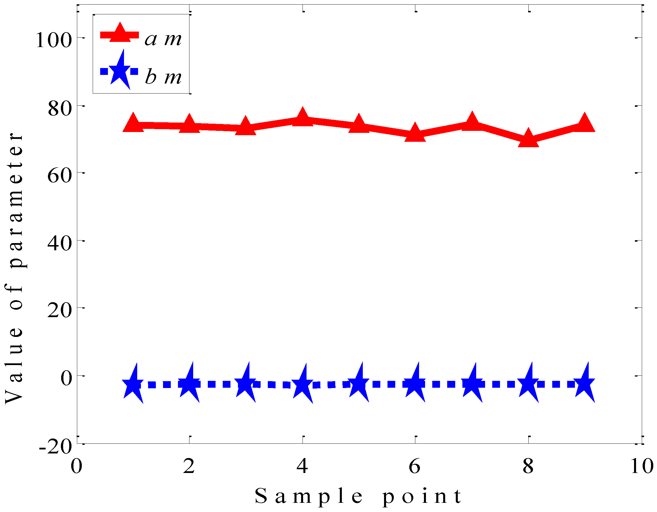
3.4. Model Parameters Estimation

AE signals were collected and recorded from tensile tests with AE instrument. There were nine samples numbered from S1 to S9. Eight samples were selected randomly as training data, while the remaining sample remained as testing data. Training data were used to estimate parameters of the elastic stage remaining time quantification model. Testing data were used to verify the effectiveness of the model. If the testing sample was S9, then the following steps should be applied to get model parameters by using training samples S1–S8.

Step 1. There are a total of eight samples in training data. According to the relationship between cumulative counts and the remaining time, the remaining time TP_i,j(t) Can be described as Equation (5):

$$T{P}_{i,j}=a_i\cdot \exp (b_i\cdot c{n}_{i.j})\begin{array}{cc}& \end{array}i=1,2,\cdot \cdot \cdot ,8\begin{array}{cc}& \end{array}j=1,2,\cdot \cdot \cdot ,n_2$$

(5)

where cn_i,j is the normalized cumulative counts; i is the sample number; j is the AE count number; a_i and b_i are parameters obtained by performing a linear least squares regression, herein, TP_i,j = TR_i,j. Therefore, eight groups of (a_i, b_i) can be obtained.

Step 2. Set cn = [1,2,…,M], herein, M = 1000. Calculate TP_i,jʹ based on Equation (5), cn, a_i and b_i. Each element in cn corresponds to 8 groups of TP_i,jʹ. Calculate the mean value of eight groups of TP_i,jʹ. The quantity of mean values is M. Then get the values of parameters am₉ and bm₉ based on calculated mean values and cn by performing a linear least squares regression. Parameters am₉ and bm₉ are taken as the parameter of sample S9. Thus, parameters am₉ and bm₉ in TPM₉,_j(t) can be obtained:

$$TP{M}_{9,j}=a{m}_9\cdot \exp (b{m}_9\cdot c{n}_{9,j})\begin{array}{cc}& \end{array}j=1,2,\cdot \cdot \cdot ,n_3$$

(6)

Step 3. Samples S1–S8 are training samples. Select samples S1–S7 to calculate a_k and b_k according to Equation (5) by performing a linear least squares regression, herein, k = 1,2,…,7, TP_k,j = TR_k,j. Calculate TP_k,jʹ based on Equation (5), cn, a_k and b_k. Each element in cn corresponds to 7 groups of TP_k,jʹ. Calculate the mean value of 7 groups of TP_k,jʹ. The quantity of mean values is M. Then get the values of parameters ad₈ and bd₈ based on calculated mean values and cn by performing a linear least squares regression. So parameters ad₈ and bd₈ in can TPD_8,j(t) be obtained:

$$TP{D}_{8,j}=a{d}_8\cdot \exp (b{d}_8\cdot c{n}_{8,j})\begin{array}{cc}& \end{array}j=1,2,\cdot \cdot \cdot ,n_4$$

(7)

Step 4. The variance between TPD_8,j(t) and TR_8,j(t) can be given by Equation (8). According to the relationship between cumulative counts and TD_8,j(t), TD_8,j(t) can be described as Equation (9):

$$T{D}_{8,j}=T{R}_{8,j}(t)-TP{D}_{8,j}(t)\begin{array}{cc}& \end{array}j=1,2,\cdot \cdot \cdot ,n_4$$

(8)

$$T{D}_{8,j}=f_8\cdot c{n}_{8,j}^2+g_8\cdot c{n}_{8,j}+h_8\begin{array}{cc}& \end{array}j=1,2,\cdot \cdot \cdot ,n_4$$

(9)

where cn_8,j is the normalized cumulative counts; f₈, g₈ and h₈ are parameters obtained by performing a linear least squares regression. Repeat Step 3 and Step 4 seven times to get (f_i, g_i, h_i); herein, i = 1,2,…,7. Hence, eight groups of (f_i, g_i, h_i) can be obtained.

Step 5. There are eight groups of (f_i, g_i, h_i). Calculate TD_i,jʹ based on Equation (9), cn, f_i, g_i and h_i. Each element in cn corresponds to eight groups of TD_i,jʹ. Calculate the mean value of eight groups of TD_i,jʹ. The quantity of mean values is M. Then get the values of parameters fm₉, gm₉, and hm₉ based on calculated mean values and cn by performing a linear least squares regression. Thus, parameters fm₉, gm₉, and hm₉ in TDM_9,j(t) can be obtained:

$$TD{M}_{9,j}=f{m}_9\cdot c{n}_{9,j}^2+g{m}_9\cdot c{n}_{9,j}+h{m}_9\begin{array}{cc}& \end{array}j=1,2,\cdot \cdot \cdot ,n_3$$

(10)

Similarly, model parameters of samples S1–S8 can be calculated according to step1–step5. Figure 5 shows the values of parameter am_l and bm_l, l = 1,2,…,9. Figure 6 shows the values of parameter fm_l, gm_l, and hm_l, l = 1,2,…,9.

Figure 5. Values of parameter am and bm.

Figure 5. Values of parameter am and bm.

Figure 6. Values of parameter fm, gm, and hm.

Figure 6. Values of parameter fm, gm, and hm.

3.5. Results and Verification of the Model

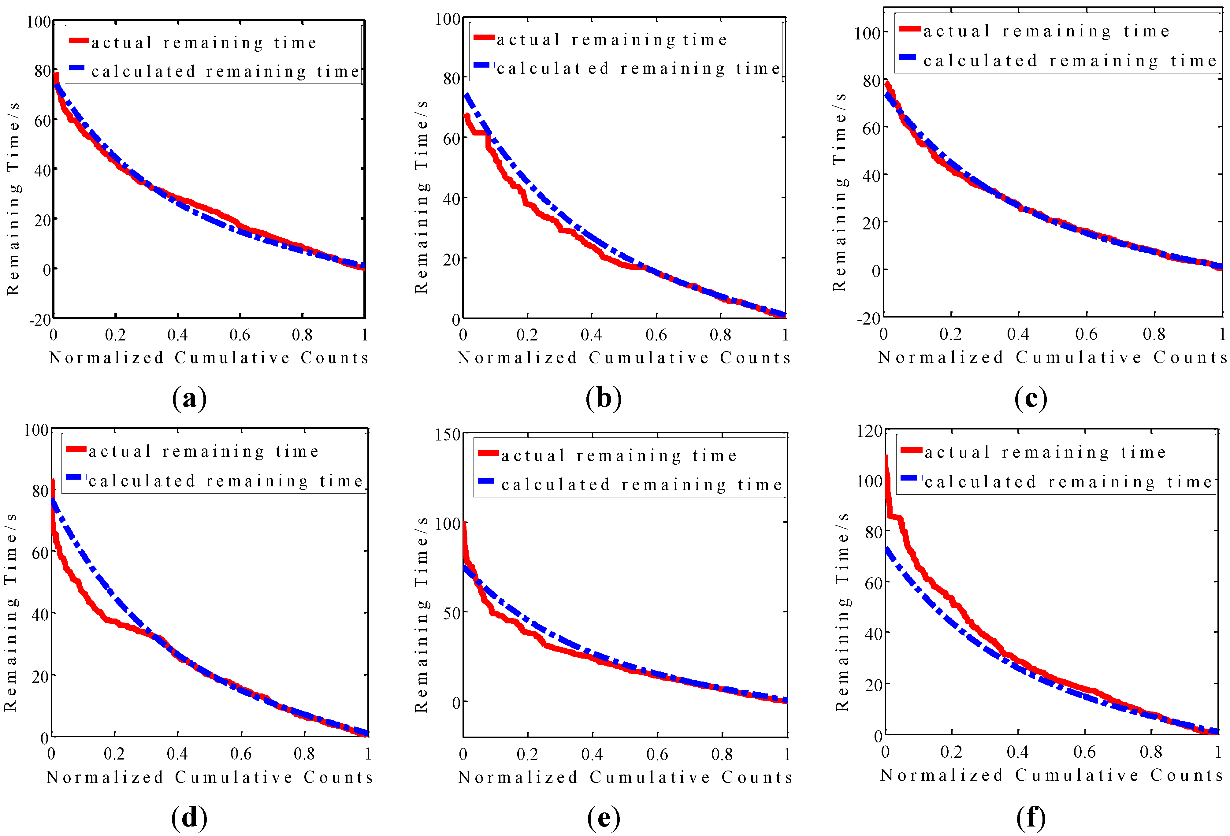
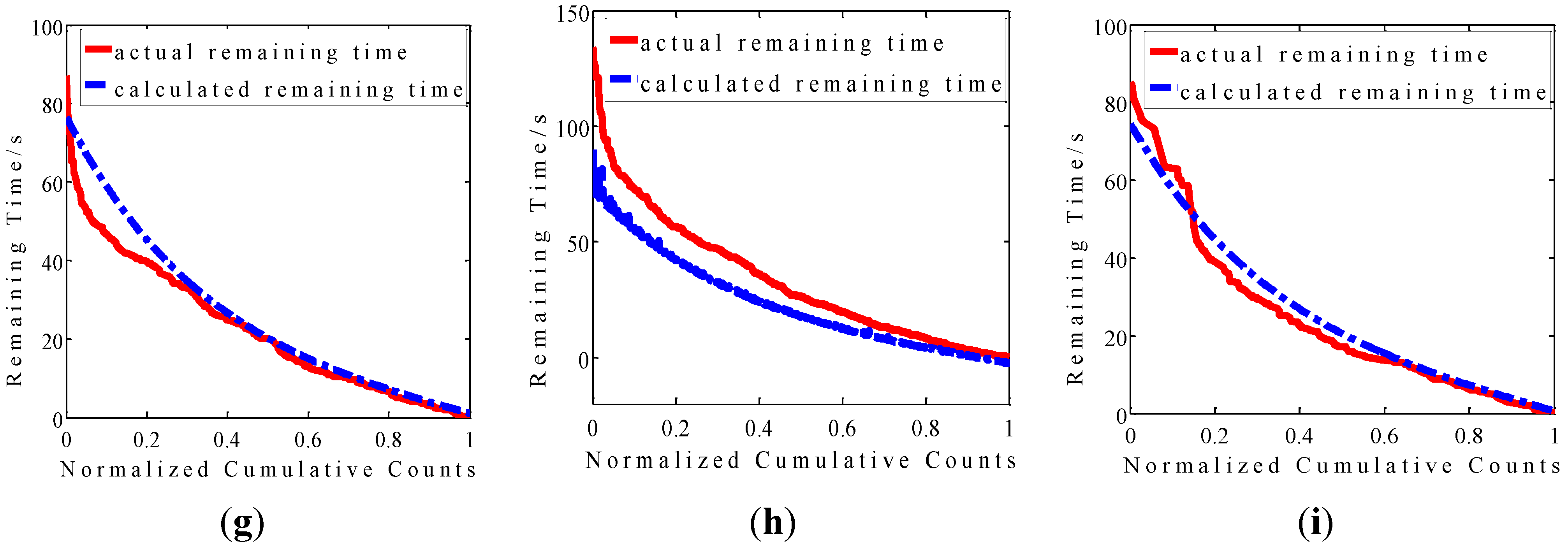
Once the values of parameter am_l, bm_l, fm_l, gm_l, and hm_l were obtained, the remaining time of samples can be calculated based on Equation (4). Figure 7 displays the comparison between the remaining time of the elastic stage calculated from AE data and actual remaining time of the elastic stage in all samples.

Figure 7. Comparison between the remaining time of elastic stage calculated from AE data and actual remaining time of the elastic stage in S1–S9. (a) S1; (b) S2; (c) S3; (d) S4; (e) S5; (f) S6; (g) S7; (h) S8; and (i) S9.

Figure 7. Comparison between the remaining time of elastic stage calculated from AE data and actual remaining time of the elastic stage in S1–S9. (a) S1; (b) S2; (c) S3; (d) S4; (e) S5; (f) S6; (g) S7; (h) S8; and (i) S9.

It is indicated in Figure 7 that the proposed model can be used to quantify remaining time of the elastic stage of high-strength aluminum alloy A356. The error between the calculated remaining time of the elastic stage and the actual remaining time is getting smaller when the material is close to the failure point.

Table 3 shows the variance between remaining time of elastic stage calculated from AE data and actual remaining time. It is indicated in Table 3 that the maximum absolute error is 59.9 s, the maximum average absolute error is 11.0 s for all samples. The average error in Table 3 refers to the mean of variance between the remaining time calculated from AE data and the actual remaining time of all the data points in each sample. Average errors of all nine tensile samples are acceptable. In other words, the proposed tensile damage quantification model is effective to quantify material tensile damage evolution of high-strength aluminum alloy A356.

Table 3. Variance between the predicted and actual remaining life.

Sample	Maximum Error/s	Minimum Error/s	Average Error/s
S1	5.7	0.001	2.0
S2	7.9	0.003	2.6
S3	4.6	0.003	1.0
S4	14.5	0.001	3.3
S5	25.0	0.144	3.4
S6	36.5	0.001	4.1
S7	14.8	0.002	3.8
S8	59.9	2.046	11.0
S9	10.8	0.224	3.2

Table 3. Variance between the predicted and actual remaining life.

Sample	Maximum Error/s	Minimum Error/s	Average Error/s
S1	5.7	0.001	2.0
S2	7.9	0.003	2.6
S3	4.6	0.003	1.0
S4	14.5	0.001	3.3
S5	25.0	0.144	3.4
S6	36.5	0.001	4.1
S7	14.8	0.002	3.8
S8	59.9	2.046	11.0
S9	10.8	0.224	3.2

4. Conclusions

In this paper, a tensile damage quantification model based on the relationship between AE counts and tensile behavior was presented to quantify material tensile damage evolution of high-strength aluminum alloy A356. Specialized tensile tests with AE monitoring were developed and carried out to verify the validity of the proposed model. Based on this study, the following conclusions can be drawn as follows:

(1)

The correlation between tensile damage and AE signals was established by characteristic parameter AC(t), which can be used to monitor material elastic deformation of tensile damage.

(2)

The proposed model is effective to quantify elastic deformation of tensile damage of high-strength aluminum alloy A356 of high-speed train gearbox shells.

(3)

Cumulative counts, as one of the most commonly-used AE parameters, can be performed in combination with the proposed model to provide warning signs for gearbox of high-speed trains when tensile damage comes to the failure point, where the final fracture will be attained quickly, and catastrophic failure may occur.

(4)

The method presented in this paper was a prognostic method only if data obtained from tensile tests is applied. In other words, the proposed elastic stage remaining time quantification model in this paper is offline. Hence, building an online elastic stage remaining time prediction model is work that needs to be done in the future.

References

1. Wang, B.M. Overall System and Bogie of High-Speed Motor Train Units; Southwest Jiaotong University Press: Chengdu, China, 2008. [Google Scholar]
2. Li, X.J. CRH bullet trains overview. Railw. Tech. Superv. 2007, 9, 26–28. [Google Scholar]
3. Yang, M.W. Acoustic Emission Testing; Machinery Industry Press: Beijing, China, 2005. [Google Scholar]
4. Haneef, T.; Lahiri, B.B.; Bagavathiappan, S.; Mukhopadhyay, C.K.; Philip, J.; Rao, B.P.C.; Jayakumar, T. Study of the tensile behavior of AISI type 316 stainless steel using acoustic emission andinfrared thermography techniques. J. Mater. Res. Technol. 2015, 137, 1–13. [Google Scholar]
5. Jalaj, K.; Sony, P.; Mukhopadhyay, C.K.; Jayakumar, T.; Vikas, K. Acoustic emission during tensile deformation of smooth and notched specimens of near alpha titanium alloy. Res. Nondestruct. Eval. 2012, 23, 17–31. [Google Scholar]
6. Luo, X.; Haya, H.; Inaba, T.; Shiotani, T.; Nakanishi, Y. Damage evaluation of railway structures by using train-induced AE. Constr. Build Mater. 2004, 18, 215–223. [Google Scholar] [CrossRef]
7. Re, V.D. Acoustic emission applications for defect detection in steels and GFRP. Int. J. Mater. Prod. Technol. 1988, 3, 38–53. [Google Scholar]
8. Chen, H.L.; Choi, J.H. Acoustic emission study of fatigue cracks in materials used for AVLB. J. Nondestruct. Eval. 2004, 23, 133–151. [Google Scholar] [CrossRef]
9. Johnson, M. Waveform based clustering and classification of AE transients in composite laminates using principal component analysis. NDT E Int. 2002, 35, 367–376. [Google Scholar] [CrossRef]
10. Lugo, M.; Jordon, J.B.; Horstemeyer, M.F.; Tschopp, M.A.; Harris, J.; Gokhale, A.M. Quantification of damage evolution in a 7075 aluminum alloy using an acoustic emission technique. Mater. Sci. Eng. A 2011, 528, 6708–6714. [Google Scholar] [CrossRef]
11. Patrik, D.; Jan, B.; Frantisek, C.; Pavel, L.; Dietmar, L.; Karl, U.K. Acoustic emission during stress relaxation of pure magnesium and AZ magnesium alloys. Mater. Sci. Eng. A 2007, 462, 307–310. [Google Scholar]
12. Godin, N.; Huguet, S.; Gaertner, R.; Salmo, L. Clustering of acoustic emission signals collected during tensile tests on unidirectional glass/polyester composite using supervised and unsupervised classifiers. NDT E Int. 2004, 37, 253–264. [Google Scholar] [CrossRef]
13. Cousland, S.M.; Scala, C.M. Acoustic emission during the plastic deformation of aluminum alloys 2024 and 2124. Mater. Sci. Eng. 1983, 57, 23–29. [Google Scholar] [CrossRef]
14. Wen, W.; Morris, J.G. An investigation of serrated yielding in 5000 series aluminum alloys. Mater. Sci. Eng. A 2003, 354, 279–285. [Google Scholar] [CrossRef]
15. Bohlen, J.; Chmelı́k, F.; Dobrŏn, P.; Kaiser, F.; Letzig, D.; Lukáč, P.; Kainer, K.U. Orientation effects on acoustic emission during tensile deformation of hot rolled magnesium alloy AZ31. J. Alloys Compd. 2004, 378, 207–213. [Google Scholar] [CrossRef]
16. Máthis, K.; Chmelík, F.; Janeček, M.; Hadzima, B.; Trojanová, Z.; Luká, P. Investigating deformation processes in AM60 magnesium alloy using the acoustic emission technique. Acta Mater. 2006, 54, 5361–5366. [Google Scholar] [CrossRef]
17. Cakir, A.; Tuncell, S.; Aydin, A. AE response of 205L SS during SSR test under potentiostatic control. Corros. Sci. 1999, 41, 1175–1183. [Google Scholar] [CrossRef]
18. Vinogradov, A.; Lazarev, A.; Linderov, M.; Weidner, A.; Biermann, H. Kinetics of deformation processes in high-alloyed cast transformation-induced plasticity/twinning-induced plasticity steels determined by acoustic emission and scanning electron microscopy: Influence of austenite stability on deformation mechanisms. Acta Mater. 2013, 61, 2434–2449. [Google Scholar] [CrossRef]
19. Kocich, R.; Cagala, M.; Crha, J.; Kozelsky, P. Character of acoustic emission signal generated during plastic deformation. In Proceedings of the 30th European Conference on Acoustic Emission Testing & 7th International Conference on Acoustic Emission, Granada, Spain, 12–15 September 2012; pp. 1–8.
20. Zhang, W.D.; Zhang, X.W.; Yang, B.; Ai, Y.B. Damage characterization and recognition of aluminum alloys based on acoustic emission signal. J. Univ. Sci. Technol. Beijing 2013, 35, 626–633. [Google Scholar]
21. Ai, Y.B.; Sun, C.; Que, H.B.; Zhang, W.D. Investigation of material performance degradation for high-strength aluminum alloy using acoustic emission. Metals 2015, 5, 228–238. [Google Scholar] [CrossRef]
22. Okafor, A.C.; Natarajan, S. Acoustic emission monitoring of tensile testing of corroded and un-corroded clad aluminum 2024-T3 and characterization of effects of corrosion on AE source events and material tensile properties. AIP Conf. Proc. 2014, 1581, 492–500. [Google Scholar]
23. Keshtgar, A.; Modarres, M. Acoustic emission-based fatigue crack growth prediction. In Proceedings of the Reliability and Maintainability Symposium: Product Quality & Integrity, Orlando, FL, USA, 28–31 January 2013; pp. 1–5.