Article

A Creep Damage Model for High-Temperature Deformation and Failure of 9Cr-1Mo Steel Weldments

by
Mehdi Basirat
1,
Triratna Shrestha
2,
Lyudmyla L. Barannyk
3,
Gabriel P. Potirniche
1,* and
Indrajit Charit
2
1
Department of Mechanical Engineering, University of Idaho, 875 Perimeter Drive, MS 0902, Moscow, ID 83844-0902, USA
2
Department of Chemical & Materials Engineering, University of Idaho, 875 Perimeter Drive, MS 3024, Moscow, ID 83844-3024, USA
3
Department of Mathematics, University of Idaho, 875 Perimeter Drive, MS 1103, Moscow, ID 83844-1103, USA
*
Author to whom correspondence should be addressed.
Metals 2015, 5(3), 1487-1506; https://doi.org/10.3390/met5031487
Submission received: 23 July 2015 / Revised: 15 August 2015 / Accepted: 17 August 2015 / Published: 21 August 2015

Abstract

:
A dislocation-based creep model combined with a continuum damage formulation was developed and implemented in the finite element method to simulate high temperature deformation behavior in modified 9Cr-1Mo steel welds. The evolution of dislocation structures was considered as the main driving mechanism for creep. The effect of void growth, precipitate coarsening, and solid solution depletion were considered to be the operating damage processes. A semi-implicit numerical integration scheme was developed and implemented in the commercial finite element code ABAQUS-Standard as a user material subroutine. Furthermore, several creep tests of modified 9Cr-1Mo steel welded specimens were conducted at temperatures between 550–700 °C and stresses between 80–200 MPa. The accuracy of the model was verified by comparing the finite element results with experiments. The comparison between the experimental and computational results showed excellent agreement. The model can be used to simulate and predict the creep-damage behavior of Cr-Mo steel components used as structural applications in power plants.

Graphical Abstract

1. Introduction

Creep failure has always been a concern in designing high temperature components and structures in coal-fired, gas-fired or nuclear power plants. The Very High Temperature Reactor (VHTR) represents the next generation of high temperature gas-cooled nuclear reactors. VHTRs would operate at the temperature range of 450–550 °C and pressures of 5–9 MPa. The target design life of the VHTR is 60+ years, and its size is almost twice as large as that of the current gas-cooled reactors. In order to satisfy the design conditions, it is necessary to employ heat and radiation resistant materials for manufacturing of the reactor pressure vessel. Manufacturing such a large pressure vessel would involve on-site ring forging and welding. During welding, the material is exposed to high temperatures which may result in local degradation of the microstructure. One potential material for such use is modified 9Cr-1Mo steel. Although 9Cr-1Mo steel exhibits excellent heat resistance, it may undergo microstructural degradation during the welding process. Moreover, during service the material would experience elevated temperatures and stresses [1]. Therefore, for applications such as pressure vessels for VHTRs, it is crucial to investigate the creep resistance of welded joints in modified 9Cr-1Mo steel, and to develop robust computational models capable of predicting the creep and fracture behavior over the range of temperatures and stresses of interest. The creep behavior of welded joints of such steel has been previously studied by several authors [2,3,4,5,6,7,8,9,10], however there is still a need for a physics-based computational model capable of predicting the creep life of welded joints over long and short service periods.
Dislocations restructuring is the main mechanism that drives creep deformation in modified 9Cr-1Mo steel. Dislocation restructuring results from dislocation and dipole generation and annihilation, as well as dislocation glide and climb. The macroscopic effect of these microstructural changes is the resulting creep strain. In addition to deformation related to changes in dislocation density, other degradation phenomena leading to creep in modified 9Cr-1Mo steel include microstructural changes involving solid solutions, precipitates, grain boundaries and subgrains. For example, the depletion of Mo atoms from the subgrain matrix under long term thermo-mechanical loading decreases the creep resistance of the steel. Moreover, coarsening of M23C6 and MX precipitates increases the spacing between the precipitates, leading to enhanced dislocation mobility. Consequently, dislocations require less energy to climb over precipitates. Void/crack nucleation and growth are some of the most important damage mechanisms in 9Cr-1Mo steel. Cavities usually nucleate at triple junctions or at the particles located on grain boundaries. Grain deformation and cavity coalescence are the main crack formation mechanism in 9Cr-1Mo [3,11,12,13].
The primary goal of this paper is to propose a unified elastic-viscoplastic constitutive model for the creep and damage evolution in modified 9Cr-1Mo steel in a format that can be implemented in the finite element method. A microstructure-based creep model combined with a continuum damage mechanics model was first developed and presented in Ref. [14]. However, in that study the model was implemented as a one-dimensional material-point simulator code, and was successfully applied only to homogenous specimens made of the base metal (BM) of modified 9Cr-1Mo steel. In the present work, the previous model was modified by considering only the generation and annihilation of dislocations as the driving mechanisms for creep. The authors observed that taking in consideration the dipole dynamics had little influence on the creep strain development. Another motivation of this paper was the need for a numerical model implementable in the finite element method to analyze three-dimensional geometries of non-homogenous materials (i.e., welded specimens) subjected to complicated loading configurations. To achieve these goals, the afore-mentioned model was modified and implemented by means of a semi-implicit integration scheme, suitable for creep simulations. The time integration algorithm was implemented in ABAQUS as a User Material Subroutine (UMAT). In order to check the accuracy and stability of the model, several case studies of elastic-viscoplastic deformations of a single element under uniaxial tensile loading have been studied. The implemented model was used to predict the creep deformation and resistance of welded joints of modified 9Cr-1Mo steel.

2. Constitutive Model

2.1. Elasticity and Creep Constitutive Equations

According to the theory of inelastic deformations, the accumulated strain is modeled as the summation of the elastic and creep strains,
ε i j = ε i j e l + ε i j c r
and in the rate form
ε ˙ i j = ε ˙ i j e l + ε ˙ i j c r
Here, the creep strain rate is assumed to be a function of equivalent stress, temperature and some internal state variables,
ε ˙ = ε ˙ ( σ ¯ , T , ξ )
where σ ¯ is the equivalent von Mises stress, defined according to the J2 plasticity theory as
σ ¯ = 3 2 S i j : S i j
where S i j = σ i j 1 3 δ i j σ k k , T represents the temperature, and ξ indicates the internal state variables.
In the present model, internal state variables refer to the dislocation density, solid solutions, precipitate size, and other strengthening mechanisms terms. These strengthening mechanisms induce isotropic hardening in the material [15]. The isotropic hardening resistance evolves during a thermally activated deformation process such as creep. In a rate-dependent inelastic deformation, the rate of evolution of the internal variables can also be expressed by the rate of change of the internal state variables ξ ˙ a . Here, ξ ˙ a is defined by some functions q a dependent on σ , T , ξ and t . Thus, the evolution of the internal state variables can be defined as
ξ ˙ a = q a ( σ ¯ , T , ξ , t )
As it was mentioned before, the decomposition rule is valid for creep deformation exposure. First the elastic response of the material will be modeled by utilizing the common linear isotropic elastic constitutive model. The widely used equation defining the linear isotropic elasticity of a material is
σ i j = 2 G ε i j e l + λ δ i j ε k k e l
where G is the shear modulus and λ is Lame’s constant.
A continuum creep-damage model was developed previously in Ref. [14]. A simplified version of the mentioned model has been employed here to analyze the creep behavior of the modified 9Cr-1Mo steel. In the original model the density of the dipole dislocations was considered when computing the creep strain accumulation. By performing numerous simulations on the original model, it was observed that neglecting the dipole dislocations density the number of equations in the model is significantly reduced, while the simulation results do not change by any sizeable amount. The literature sources and a detailed description of the governing equations in the constitutive model for creep deformation were presented in Ref. [14]. Here, only a summary of the main governing equations is presented.
The creep strain rate in a material can be evaluated by using with the Orowan’s equation modified for the presence of damage,
ε ¯ ˙ c r = ρ m b B visc M D ( σ ¯ α M C G b ρ m )
In this equation ρ m is the mobile dislocation density, Bvisc is the dislocation mobility term which are the dependent variables and b is the Burger’s vector, α is a dislocation interaction constant, M is the Taylor factor, C is the inelastic deformation factor (C was taken 0.2 in this study), which are all independent variables. To simplify notations, the following constant is introduced K1 = αMCGb. In Equation (7), D represents the total damage caused by the cumulative effects of precipitate coarsening, depletion of solid solutions, and void and crack formation. The dislocation mobility term is defined as
B visc = 9 Ω D sol K B T M C G 2 0 b 7 ε a 2 ln ( r 2 r 1 )
where Ω is the atomic volume (considered here as equal to b 3 ), KB is the Boltzmann constant, T is the temperature, Dsol is the solute atom diffusion coefficient in solvent atoms, C0 is the solute concentration, r1 and r2 are the outer and inner cut-off radii of the dislocation stress field, and εa is the relative size misfit between solute and solvent atoms [16]. The rate of evolution of mobile dislocations density is defined as the difference between the rate of generation of mobile dislocations ( ρ ˙ m , gen ), and the rate of annihilation of mobile dislocations density ( ρ ˙ m , ani ),
ρ ˙ m = ρ ˙ m,gen ρ ˙ m,ani
Based on the results reported in [14], it can be shown that the rate of generation of the mobile dislocation can be computed as
ρ ˙ m , gen = ρ m B visc ρ m k λ D ( σ ¯ K 1 ρ m )
where kλ is a material parameter that depends on temperature and equivalent stress. Similarly, it can be shown that the rate of annihiliation of the mobile dislocations is
ρ ˙ m,ani = 4 M ε ˙ d dip ρ m b n g
where d dip is the dipole formation distance [16]. The annihilation rate of mobile dislocations is given by the summation of the densities of dislocations which annihiliate spontaneously and that of the dislocations that form dipoles. It is a function of the strain rate, the mobile dislocations density, the Burger’s vector, the Taylor factor and the number of active slip planes n g . Replacing ε ˙ in Equation (11) by its value from Equation (7), the rate of annihilation of mobile dislocations can be expressed as
ρ ˙ m,ani = 4 d dip ρ 2 m B visc n g D ( σ ¯ K 1 ρ m )
As two mobile dislocations of opposite sign approach each other within a certain distance, d dip , they form dipoles and produce sessile dislocations. d dip is calculated as
d dip = M 8 π ( 1 ν ) G b σ ¯
In this equation, ν is the Poisson’s ratio. Replacing d dip in Equation (12), the rate of annihilation of mobile dislocations becomes
ρ ˙ m,ani = 4 M b G ρ 2 m B visc 2 π ( 1 ν ) n g D σ ¯ ( σ ¯ K 1 ρ m )

2.2. Damage Constitutive Equations

The material microstructure will degrade during high temperature exposure, which means that the strengthening mechanisms will become less effective during creep loading. The main strengthening mechanisms in modified 9Cr-1Mo steel are work hardening, solid solution strengthening, precipitation hardening, and subgrain boundary strengthening. It has been shown by several researchers that Mo atoms in solid solution precipitate to form coarse Laves-phase particles under long term thermo-mechanical loading [17,18,19]. Moreover, the precipitate (M23C6 and MX) coarsening in modified 9Cr-1Mo increases the inter-particle spacing between precipitates. Solid solutions depletion and precipitate coarsening increase the dislocations mobility. Consequently dislocations require less energy to move. Furthermore, void nucleation and crack formation is one of the most important creep damage mechanisms in 9Cr-1Mo steel. The cavities usually nucleate at triple junctions or at particles located on grain boundaries. Grain deformation and cavity coalesce are the main crack formation mechanisms in 9Cr-1Mo steel.
Mo is added to 9Cr-1Mo steel to induce solid solution strengthening. During creep loading, depletion of Mo atoms occurs in the subgrain matrix, leading to the precipitation of Fe2Mo Laves phases. It has been shown by experiments that Fe2Mo precipitates with low volume fraction and larger size could not effectively block dislocation motion during creep. These large size Laves phases (Fe2Mo) are a source for dislocations absorption, and they are brittle phases. These inopportune properties lead to a reduction of the creep resistance of modified 9Cr-1Mo [11].
The following equations show the damage caused by solid solution depletion and its corresponding rate.
D s = 1 C ¯ t C 0
D ˙ S = K S D S 1 / 3 ( 1 D S )
Here Ds is the damage term represented by the solid solution depletion, and is a function of the initial and current solid solution concentrations, C 0 and C t , respectively, and K S is a material constant.
Another important damage mechanism in 9Cr-1Mo steel is caused by the coarsening of M23C6 and MX precipitates. The coarsening of precipitates increases the interparticle spacing, and consequently the easier motion of dislocations (in the case of MX). It also enhances recovery, i.e., subgrain coarsening (in case of M23C6), which means less creep resistance. The damage and damage rate, accounting for the precipitate coarsening, are written as
D P = 1 P 0 P t
D ˙ p = K p ( 1 D p ) 4
where P 0 and P t are the initial and current size of the precipitates, respectively, and K P is a material constant.
A leading failure mechanism during the creep deformation of modified 9Cr-1Mo is crack nucleation and growth. Microstructural stress concentrations are responsible for grain boundary sliding leading to the formation of creep cavities and creep crack formation. Creep crack formation and growth has been extensively studied in the literature [20]. In this paper, a modified Kachanov damage model has been employed for the crack-driven creep damage. Simply, creep damage is expressed as a function of the creep exposure time (t), the creep rupture time trupture, and a material constant B, which is a function of the applied stress. The rupture time can be obtained from experiments. The dependence of rupture time on the applied stress for the 9Cr-1Mo steel welded specimens tested in this study is shown in Figure 1.
Figure 1. True stress versus creep rupture time for modified 9Cr-1Mo 91 steel specimens [1].
Metals 05 01487 g001
The crack-driven damage term is modeled as
D N = 1 ( 1 t t rupture ) 1 / ( 1 + B )
To summarize, the total damage in the material caused by solid solution depletion, precipitate coarsening and crack formation is denoted as D , and is defined as
D = D ( D S , D P , D N ) = ( 1 D S ) ( 1 D P ) ( 1 D N )

3. Numerical Implementation

The analytical model presented in the previous section was implemented in the finite element code ABAQUS Standard as a User Material (UMAT) subroutine. Creep deformation is a history-dependent process. In order to solve the set of governing differential equations for the constitutive model, it is necessary to discretize these equations and integrate them over time.
First, the governing equations for the equivalent stress are presented. The elastic strain at time step n + 1 is calculated from its value at the previous time step n and its increment,
ε i j , n + 1 el = ε i j , n el + ( Δ ε i j tr Δ ε i j cr )
Replacing Equation (21) in Equation (2) and after some algebra, the stress in the predictor-corrector format can be written as
σ i j = σ i j tr 2 G Δ ε i j cr
According to the classical J2 theory of plasticity, it is possible to express the components of the creep strain rate in the direction of stress as
ε ˙ i j cr = λ S i j = 3 2 ε ¯ ˙ cr S i j σ ¯
where λ = 3 ε ¯ ˙ cr 2 σ ¯ is the creep strain multiplier. Multiplying the above equation by the time increment Δt one obtains
Δ ε i j cr = 3 2 Δ ε ¯ ˙ S i j σ ¯ Δ t = 3 2 Δ ε ¯ cr S i j σ ¯ = n Δ ε ¯ cr
In the above equation, n is the unit vector normal to the yield surface, and the above equation represents the normality rule. It can be shown that n = 3 2 S i j σ ¯ . With some modifications, it is possible to rewrite Equation (22) in an equivalent stress format presented by [21]
σ ¯ σ ¯ tr + 3 G Δ ε ¯ cr = 0
The above formula is the governing equation for the equivalent creep stress, while the trial stress σtr is calculated using Equation (6).
In addition to the creep strain, another state variable considered in this model is the density of mobile dislocations ρm. Replacing Equations (10) and (14) in Equation (9), the evolution rate of mobile dislocation density becomes
ρ ˙ m = g ( σ ¯ , ρ m , D ) = ρ m B visc ( σ ¯ K 1 ρ m ) D ( ρ m K Λ 4 d dip ρ m n g )
In the current model, the integration of the damage term is performed using an explicit scheme. The following equations show the discretized form of Equations (25) and (26)
F ( σ ¯ n + 1 , ρ m n + 1 , D n ) = σ ¯ n + 1 σ ¯ n + 1 Tr + 3 G f ( σ ¯ n + 1 , ρ m n + 1 , D n ) = 0
G ( σ ¯ n + 1 , ρ m n + 1 , D n ) = ρ m n + 1 ρ m n + g ( σ ¯ n + 1 , ρ m n + 1 , D n ) = 0
To solve the above system of equations, the Newton-Raphson (N-R) method combined with a line search algorithm was used. The Jacobian matrix needed in the N-R method was computed numerically, however, an analytical form of the Jacobian matrix could also be easily obtained. At the end of each time step, the damage terms have been explicitly updated. The N-R method gives the increments in equivalent stress and dislocation density
( Δ σ ¯ n + 1 Δ ρ m n + 1 ) = ( F σ ¯ n + 1 F ρ m n + 1 G σ ¯ n + 1 G ρ m n + 1 ) 1 ( F ( σ ¯ n , ρ m , D T n 1 ) G ( σ ¯ n , ρ m n , D T n 1 ) )
while σ ¯ n + 1 , and ρ m n + 1 are updated according to σ ¯ n + 1 = σ ¯ n + Δ σ ¯ n + 1 , and ρ m n + 1 = ρ m n + Δ ρ m n + 1 . The total damage D at time step n + 1 is updated using Equation (20) in which each of the damage terms DS, DP, and DN are used with their values at step n + 1. DS and DP are updated according to D n + 1 = D n + D ˙ n Δ t , and DN is updated according to Equation (19). Introducing the updated variables and Dn+1 in Equation (31), ε ¯ ˙ n + 1 cr is computed,
ε ¯ ˙ n + 1 cr = f ( σ ¯ n + 1 , ρ m n + 1 , D n + 1 ) = ρ m n + 1 b B visc M D n ( σ ¯ n + 1 α M C G b ρ m n + 1 )
and Δ ε ¯ cr = ε ¯ ˙ n + 1 cr Δ t . Substituting the equivalent increment of creep strain Δ ε ¯ cr in Equation (23), the components of creep strain tensor are calculated. Once the strain increment and strain tensors components are computed, the stress increment and stress tensor components will be obtained using the following equation
σ i j n + 1 = C el ( Δ ε i j n + 1 tr Δ ε i j cr ) + σ i j n
The updated stress, internal state variables and the tangent stiffness matrix are returned to ABAQUS by the UMAT. The elastic stiffness matrix C el was used to update the tangent stiffness matrix, which is a common approach for finite element simulations of creep deformation [22].

4. Experiments

Creep experiments were conducted on welded specimens at temperatures between 550 °C and 700 °C and stress levels between 80 and 200 MPa, by using an Applied Test Systems (ATS, Butler, PA, USA) lever arm (20:1) creep tester. Welded specimens were made of ASTM A387 Grade 91 CL2 steel (Grade 91) steel. The specimens were machined out of as-received plates, and were given a round cross-section with a diameter of 12.7 mm and gage length of 45 mm. The chemical composition of Grade 91 steel is indicated in Table 1.
Table 1. Chemical composition (wt. %) of modified 9Cr-1Mo steel.
ElementsNominalMeasured
Cr8.00–9.508.55
Mo0.85–1.050.88
V0.18–0.250.21
Nb0.06–0.100.08
C0.08–0.120.1
Mn0.30–0.600.51
Cu0.4 (max.)0.18
Si0.20–0.500.32
N0.03–0.070.035
Ni0.40 (max.)0.15
P0.02 (max.)0.012
S0.01 (max.)0.005
Ti0.01 (max.)0.002
Al0.02 (max.)0.007
Zr0.01 (max.)0.001
FeBalanceBalance
The as-received plates were delivered from hot rolled Grade 91, in normalized and tempered condition (i.e., austenitized at 1038 °C for 240 min, followed by air cooling, and tempered at 788 °C for 43 min). The original dimensions of the as-received Grade 91 plate were 104 mm × 104 mm × 12.7 mm. The mechanical properties of the material are shown in Table 2.
Table 2. Mechanical properties of modified 9Cr-1Mo steel.
Yield Strength (MPa)Tensile Strength (MPa)Elongation
Gage Length (mm)%
53368350.8026.0
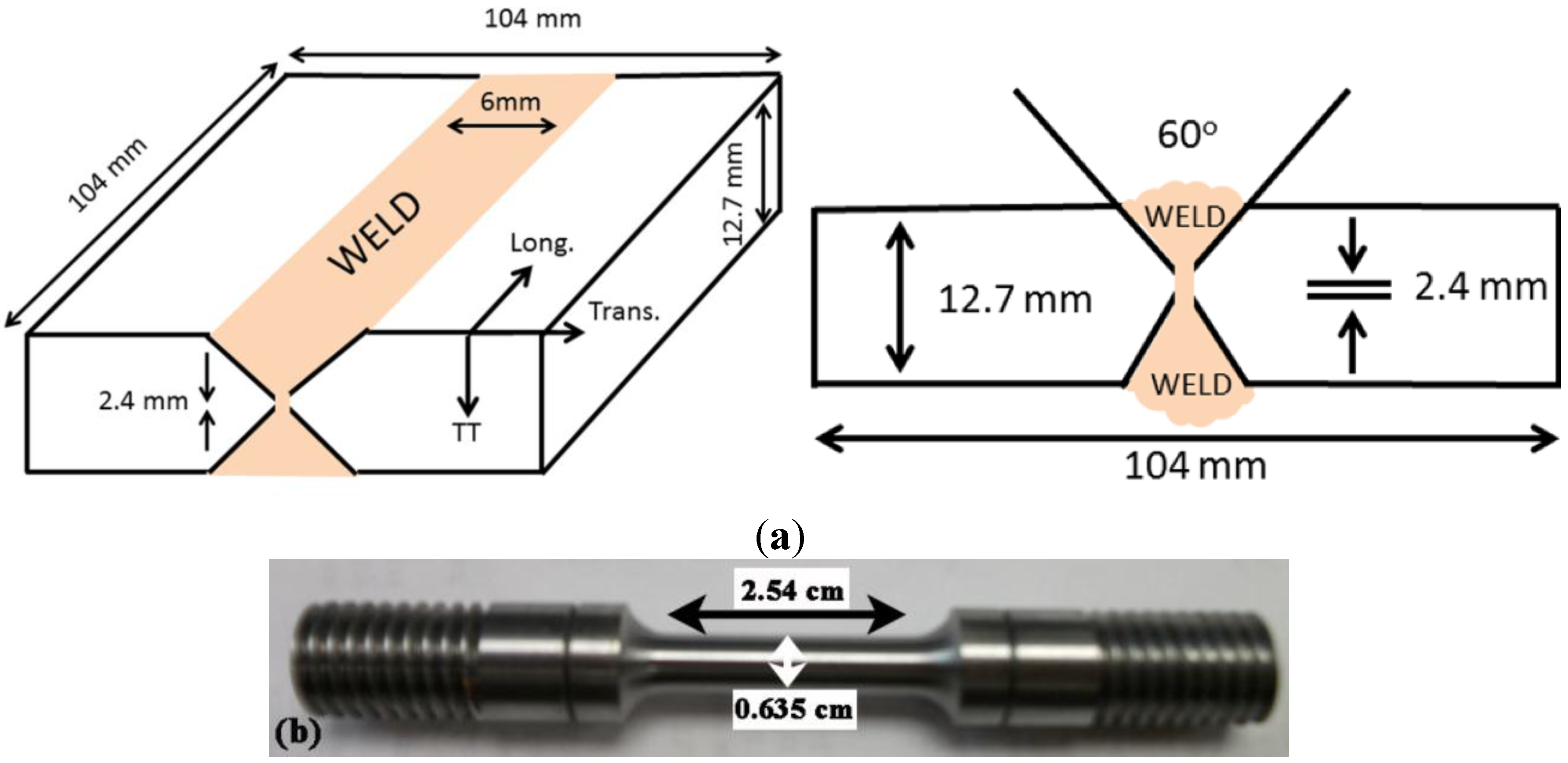
In order to machine the specimens, plates were cut into halves and tapered for double V welding joints, as shown in Figure 2.
Figure 2. (a) Schematic representation of the double V-butt welded plate; and (b) specimen used for creep testing. The specimen is cut from the plate, and the central portion of the specimen matches the weld zone.
Metals 05 01487 g002
In this figure, Long, Trans, and TT are the longitudinal, the transversal and the through-thickness directions, respectively. The Metrode 2.4 mm diameter 9CrMoV-N TIG filler wire, which is well known for low residual stresses, was used for welding. The plates were preheated at 260 °C before welding. To prevent overheating, the steel plates were placed on an aluminum plate during welding. The welding was completed in three successive passes with a current of 130 A and voltage of 15 V. The post-weld heat treatment (PWHT) was conducted at 750 °C for 2 h.
As it was mentioned earlier, the microstructure of the welding heat affected zone will undergo changes due to the temperature gradient during welding. The microstructure of the as-welded and post-weld heat-treated specimens exhibits three different zones, i.e., the unaffected base material, the heat affected zone and the weld material. A typical heat affected zone presents two distinct microstructures: the fine grain heat affected zone (FGHAZ), and the coarse grain heat affected zone (CGHAZ). It has been widely reported that type IV cracks initiate in the HAZ, being caused by the non-uniform structure of the HAZ. The non-uniform structure of HAZ is caused by the partial transformation of austenite into martensite, the presence of retained austenite, the formation of delta-ferrite, and differential migration of interstitial and precipitate forming elements through the heat affected zone which creates a complex microstructure prone to failure.
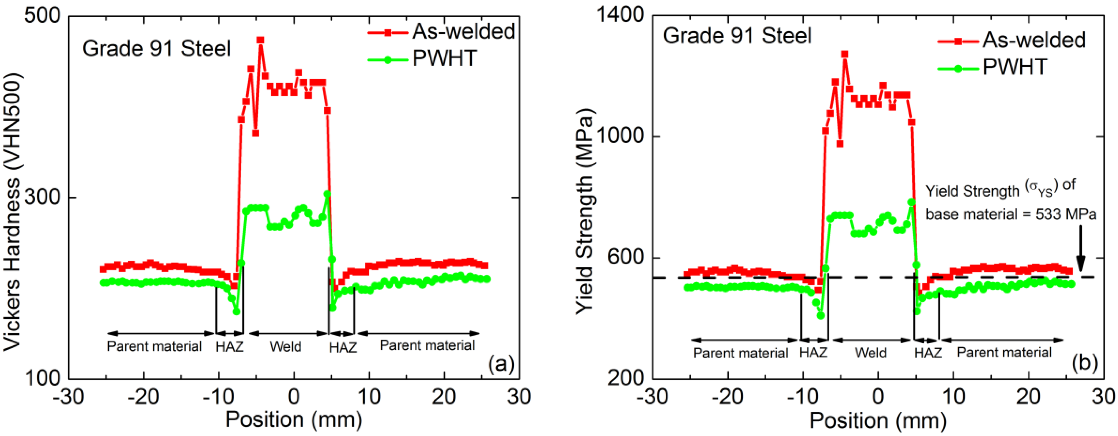
The hardness of Grade 91 steel in the as-received and PWHT condition was measured using a Vickers microhardness tester (LECO, St. Joseph, MI, USA). The hardness of the as-welded material increased across the weld but decreased in the HAZ, as shown in Figure 3a. The as-welded specimen had a maximum hardness of 474 VHN in the weld, while HAZ exhibited the lowest hardness of 200 VHN. The base material had a hardness of approximately 225 VHN. The HAZ was symmetric on either side of the weld. The hardness profile of specimen PWHT at 750 °C for 2 h was similar to the as-welded specimen, but the hardness magnitudes were lower. The maximum hardness of 304 VHN was observed in the weld, while the lowest hardness of 174 VHN was observed in the HAZ. The hardness of steels can be correlated with the yield stress, thus the yield stress profile of the as-welded and PWHT specimens is similar to the hardness profile, as illustrated in Figure 3b.
Figure 3. Vickers microhardness (a); and yield strength profile (b) of welded Grade 91 steel. Position “0” indicates the center of the weld.
Metals 05 01487 g003

5. Results and Discussion

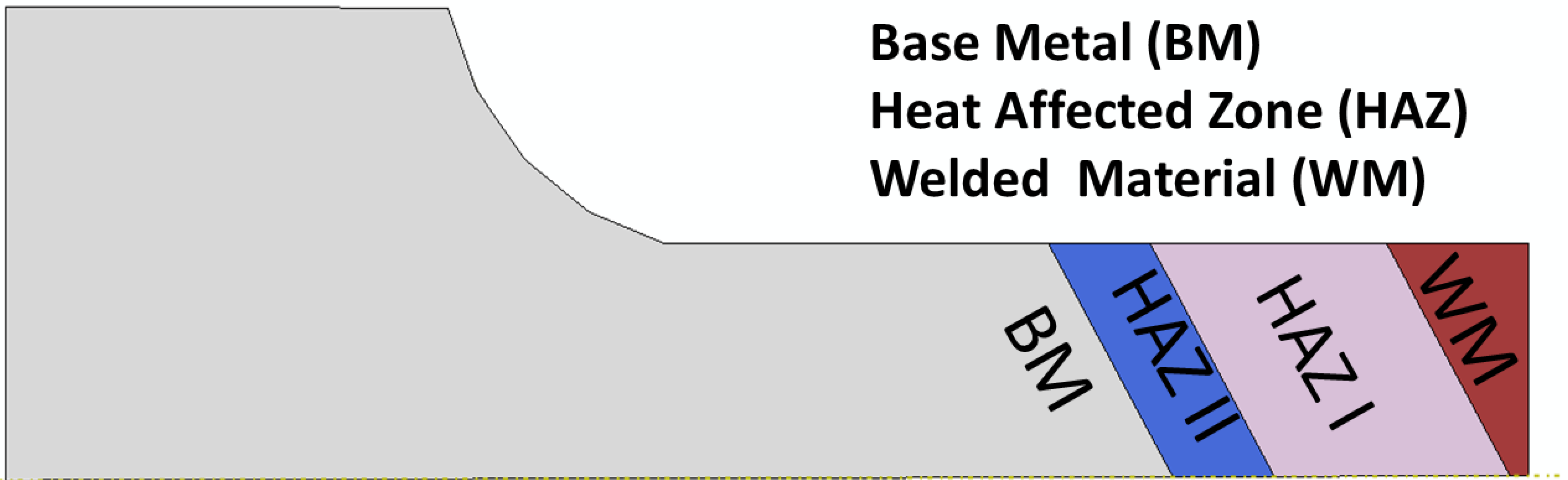
To perform a finite element analysis on the welded specimen, one needs to obtain accurate material constants in the constitutive model for each distinct region of the specimen. In general, it is reasonable to divide the specimen into four regions, the BM, FGHAZ (HAZ II), CGHAZ (HAZ I) and the welded material (WM). Although the HAZ microstructure changes gradually from the WM to the BM, for simplicity, in this study the HAZ was considered as divided into two separate and homogeneous zones (HAZ I and HAZ II). In a study by Gaffard et al. [3], it was shown that the WM and BM demonstrate similar steady state creep behaviors. Hence, the same material properties were considered for the BM and WM regions in the finite element model. Simulations were performed on a model with three materials, the BM and two HAZ regions. The HAZ segment was divided into HAZ I and HAZ II. Figure 4 shows a schematic of each segment of the welded specimen.
Figure 4. Schematic representation of the welded specimen, showing the Base Metal (BM), Heat Affected Zone I and II (HAZ I and II), and the Welded Material (WM).
Metals 05 01487 g004
Given such a configuration of the specimen, the steady state creep rate is computed using the following equation
ε ˙ SS l T = l BM ε ˙ BM + l WM ε ˙ WM + l HAZ ε ˙ HAZ
where, ε ˙ SS , ε ˙ BM , ε ˙ WM and ε ˙ HAZ are the steady state creep strain rates of the welded specimen SS, BM, WM, and HAZ, respectively. l T (=45 mm) is the total gage length of the specimen, l BM , l WM ( l BM + l WM = 39 mm) represent the length of BM, WM zones, and l HAZ (=6 mm) is the length of HAZ zone. If the steady state creep test data for both welded specimen and BM are available, the material properties for HAZ can be obtained. Considering the same material properties for the steady state creep rate of the welded specimen in the WM and BM, Equation (32) is used to compute the creep rate developed in the HAZ as
ε ˙ HAZ = ε ˙ SS l T ( l BM + l WM ) ε ˙ BM l HAZ
As discussed before, the model requires a number of material constants. Some of them depend on temperature and applied stress, while others are independent of stress and temperature. The material properties independent of the testing conditions are b = 2.47 e 10 m , M = 3 , n g = 5 , α = 0.02 , and C 0 = 0.056 . Two key material parameters for the second stage creep are k λ and ρ m . While it is not straightforward to measure the dislocation density ρ m , it has been showed by [14] that if the initial dislocation density is in a realistic range (i.e., between 0.2 × 10¹⁴ and 2.0 × 10¹⁴ m−2), the results will converge to approximately the same value [14]. The values for k λ 
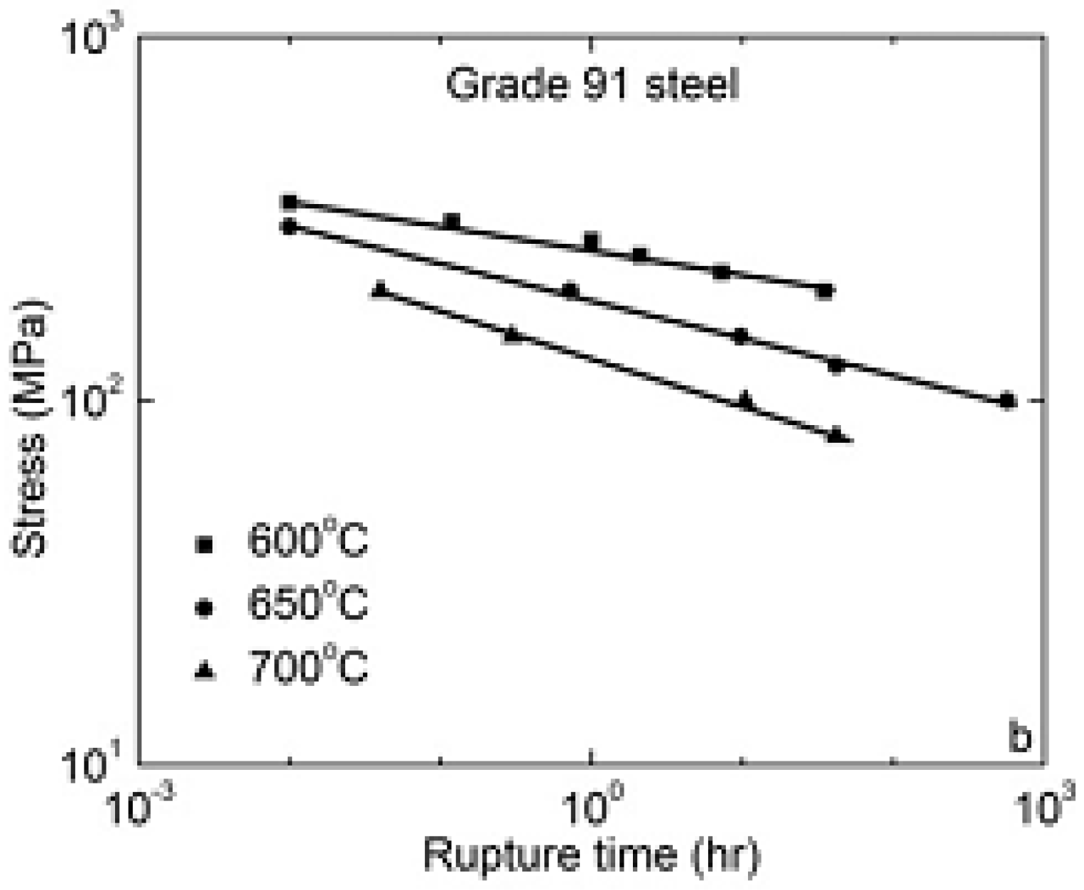
may be determined by performing simulations for the minimum creep rate in the welded and BM specimens, and by employing Equation (33). Furthermore, t rupture for different loading conditions has been obtained from experiments, and is illustrated in Figure 1. Values for the remaining material constants used in this study are presented in Table 3.
Table 3. Material constants used in the constitutive model.
MaterialTemperaturesConstantσ = 100 MPaσ = 150 MPaσ =200 MPa
BM & WM600 °Ckλ1 × 10455090
HAZ I650 °C30025.512
HAZ II700 °C100149
HAZ I600 °CKs-5.6 × 10−92.7 × 10−6
650 °C0.8 × 10−45.5 × 10−90.8 × 10−4
700 °C-0.8 × 10−40.8 × 10−4
HAZ II600 °CKp-1.9 × 10−61.9 × 10−6
650 °C0.1 × 10−50.2 × 10−60.6 × 10−3
700 °C-0.1 × 10−50.1 × 10−5
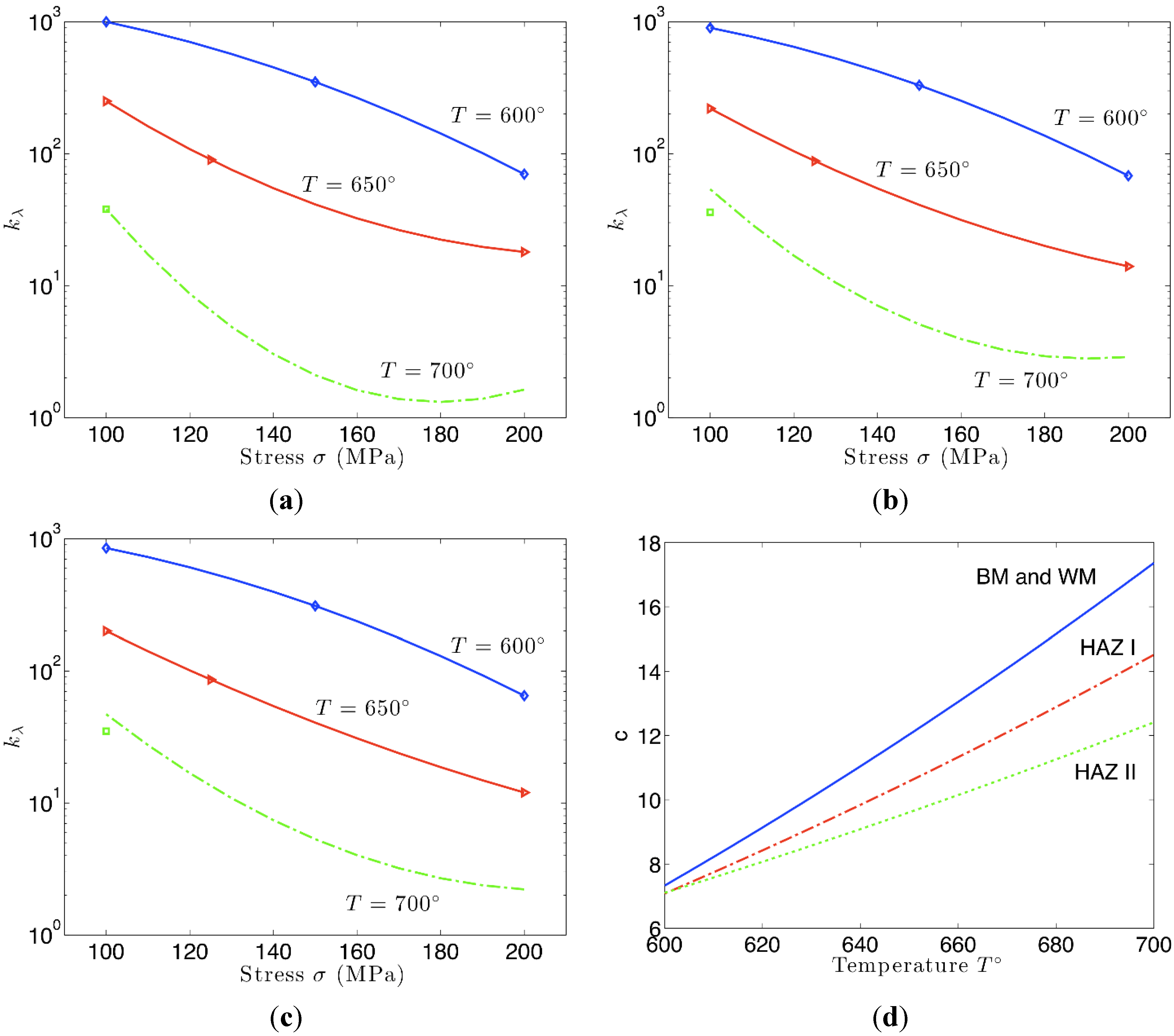
To perform predictions at temperatures different than those that have been tested in this study, it is useful to perform curve-fitting of material parameters versus temperature. For example, kλ is chosen because it is a key material constant in this model. By studying the values of kλ in Table 3, which were obtained from numerical simulations for each specimen microstructure (BM and WM, HAZ I and HAZ II), it is proposed that ln(kλ) can be modeled as a quadratic function of σ with coefficients a, b, and c dependent on temperature T, namely
ln ( k λ ) = a ( T ) σ 2 + b ( T ) σ + c ( T )
where a(T), b(T), and c(T) are different for each zone of the material and they need to be determined. Three values of kλ are available at three values of stress σ at temperatures T = 600 °C and T = 650 °C, and only one value is known at T = 700 °C, due to the available experimental data. The results of fitting ln(kλ) to a quadratic polynomial for T = 600 °C and T = 650 °C are shown in Figure 5a,b using solid lines, while the symbols represent values from the simulations.
Figure 5. Logarithmic plot of kλ as a function of stress for T = 600 °C, 650 °C and 700 °C for (a) BM and WM, (b) HAZ I and (c) and HAZ II. (d) Quadratic curve-fitting of coefficient c. Solid curves represent fitted lines, while dash-dotted curve is the extrapolation for temperature T = 700 °C.
Metals 05 01487 g005
Thus, we know a(T), b(T), and c(T) at T = 600 °C and T = 650 °C. To find the coefficients a, b and c at T = 700 °C and describe kλ as a function of temperature, we assume that a, b and c depend quadratically on T as well, i.e.,
a ( T ) = α 2 T 2 + α 1 T + α 0   b ( T ) = β 2 T 2 + β 1 T + β 0   c ( T ) = γ 2 T 2 + γ 1 T + γ 0
Requiring that a, b and c assume the computed values at T = 600 °C and T = 650 °C as well as using the table value of kλ at σ = 100 MPa and T = 700 °C in Equation (34) produces a linear 10 × 12 underdetermined system for unknowns αi, βi, γi, i = 1, 2, 3 and a(T), b(T), c(T) at T = 700 °C. The system was solved in a least squares sense using the truncated singular value decomposition (SVD) method because of ill-conditioning of the coefficient matrix. As an example, in Figure 5d coefficient c is shown as a quadratic function of T for different zones of the welded specimen. It was found that c = 17.366 at T = 700 °C for BM and WM, c = 14.517 for HAZ I and c = 12.414 for HAZ II. Coefficients a and b are much smaller (a ~ 10−4, a ~ 10−1) and they can be approximated at T = 700 °C in a similar manner. With a, b and c known at T = 700 °C, kλ at T = 700 °C can be reconstructed using Equation (34). The results of such reconstruction for each material are shown with a dashed line in Figure 5. These approximated curves provide an excellent agreement with a value of kλ available at T = 700 °C and σ = 100 MPa.
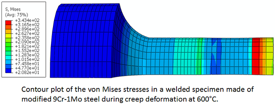
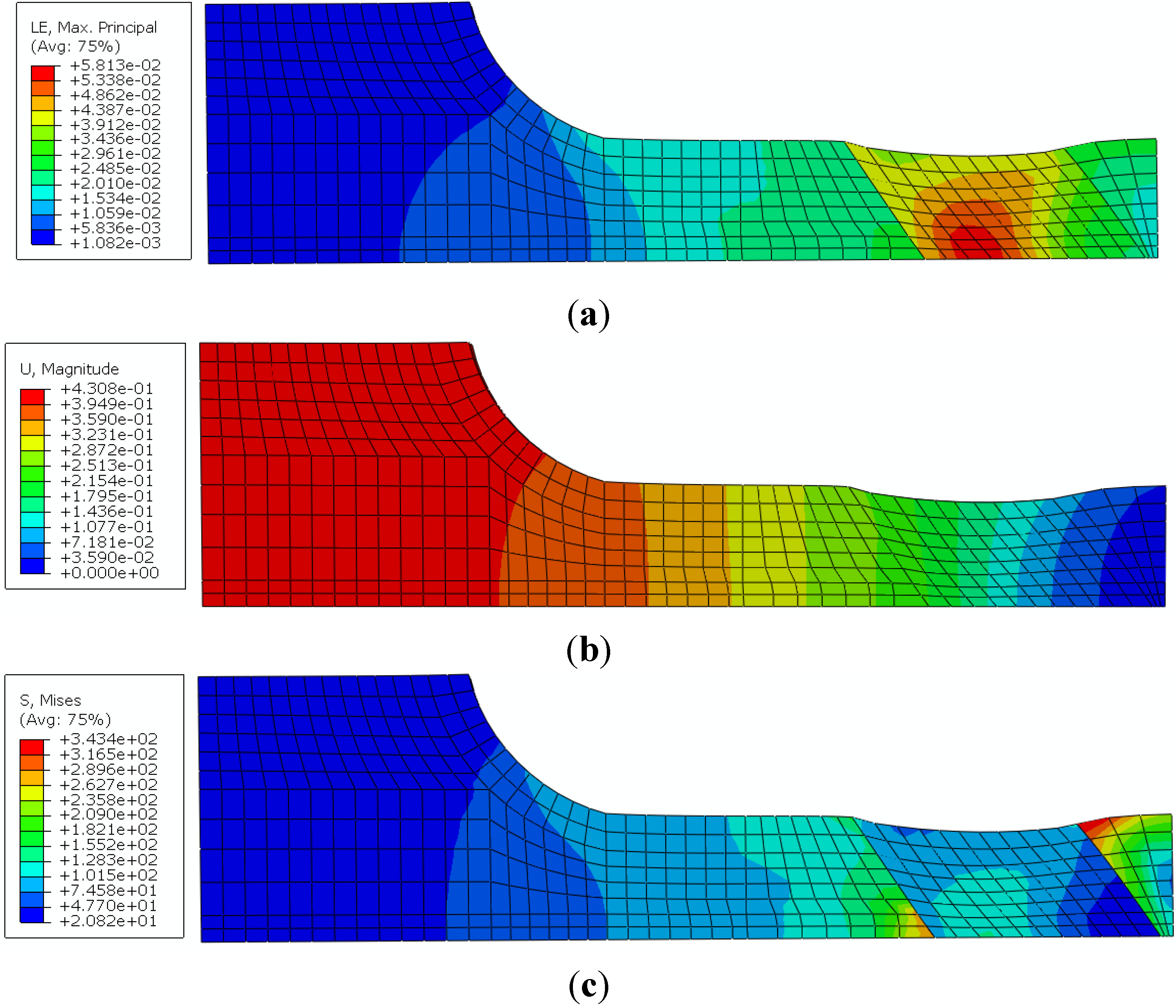
Finite element simulations have been performed in ABAQUS for a range of stresses and temperatures. 
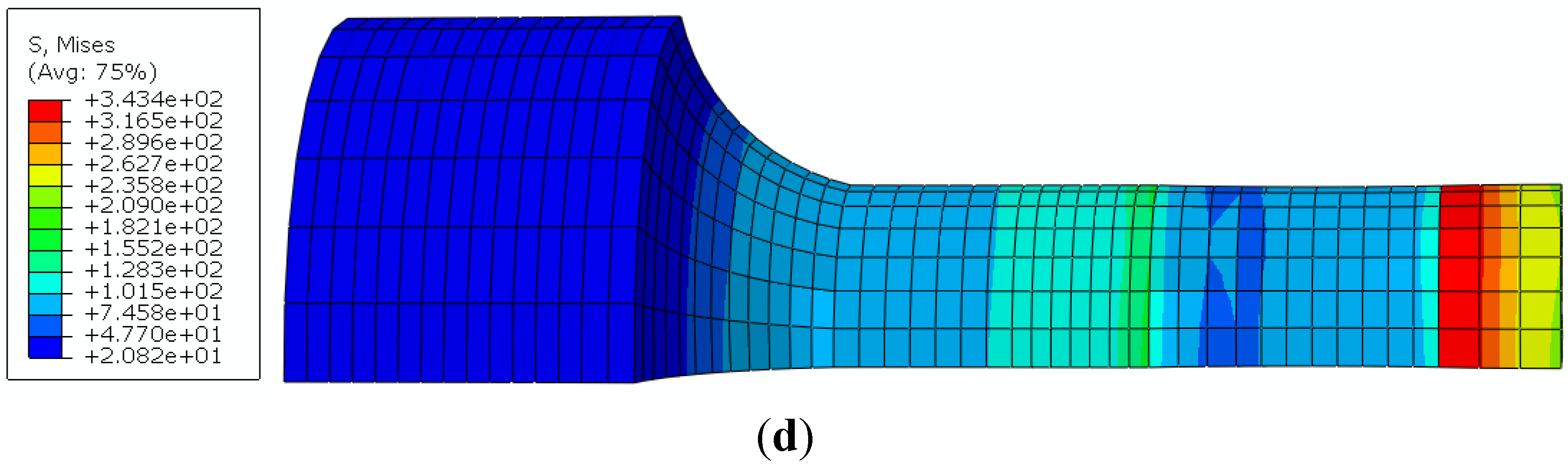
Figure 6a–d show the displacement along the axis of the specimen, the maximum principal strain, and the von-Mises stress on a cross-section and at the surface of the specimen, respectively.
Figure 6. Finite element simulations of creep in a welded 9Cr-1Mo specimen subjected to an applied stress of 200 MPa and at a temperature of 600 °C: (a) maximum principal strain; (b) displacement along the axis of the specimen; (c) von-Mises stress in the cross section of the specimen; and (d) the stress distribution at the surface of the specimen.
Metals 05 01487 g006aMetals 05 01487 g006b
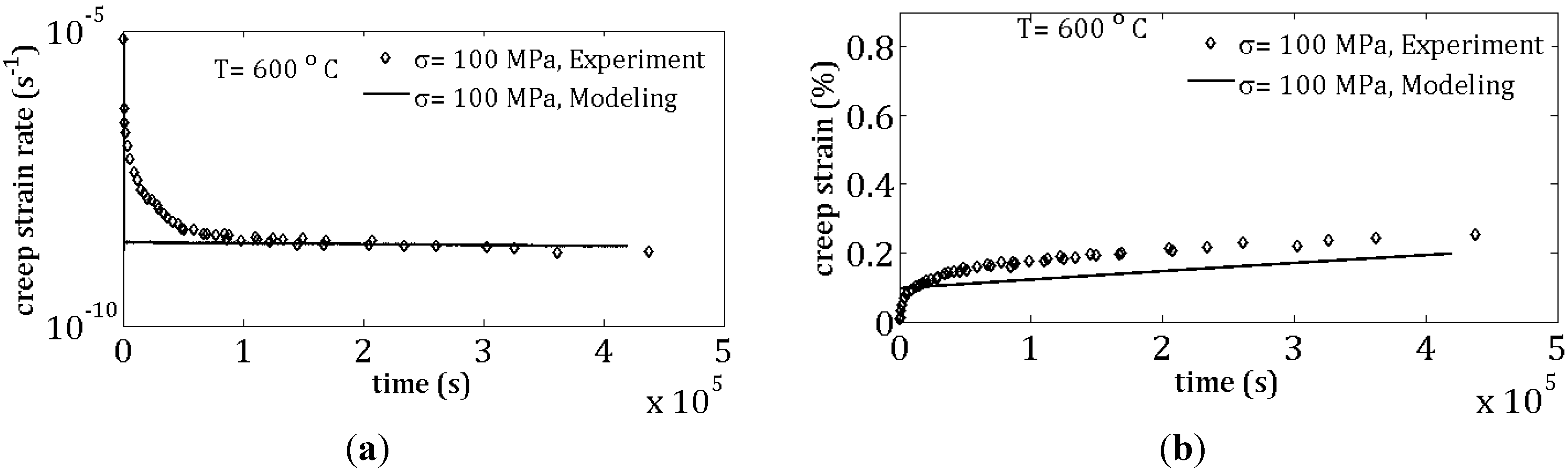
Figure 7 shows the comparison of the experimental result to the model simulation for 100 MPa and 600 °C. Figure 7a shows the rate of creep strain versus time, and Figure 7b shows the true creep strain versus time.
Figure 7. Creep results from experiments and finite element simulation for 100 MPa and 600 °C: (a) creep strain rate versus time; and (b) true creep strain versus time.
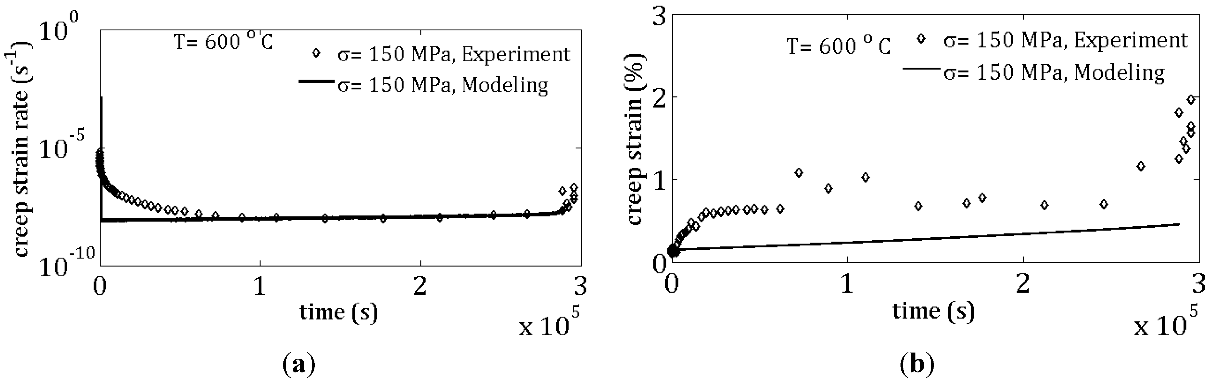
Metals 05 01487 g007
Figure 8. Creep results from experiments and finite element simulation for 150 MPa and 600 °C: (a) creep strain rate versus time; and (b) true creep strain versus time.
Metals 05 01487 g008
The simulation and experimental results comparison for 150 MPa at 600 °C have been shown in Figure 8. Again, Figure 8a is the creep strain rate versus time and Figure 8b is the true creep strain versus time.
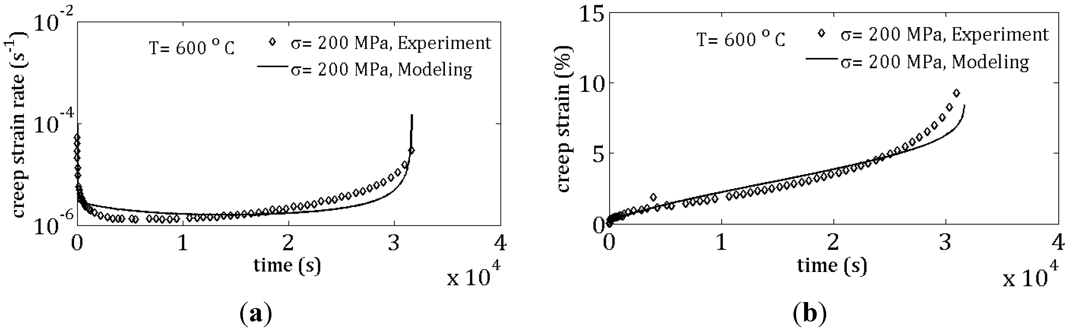
For specimen crept at 200 MPa and 600 °C Figure 9a,b, respectively, show the creep strain rate versus time and the true creep strain versus time.
The comparisons of the modeling versus experiments at 650 °C and applied stresses of 100 MPa, 125 MPa and 200 MPa are shown in Figure 10, Figure 11 amd Figure 12, respectively.
Figure 9. Creep results from experiments and finite element simulation for 200 MPa and 600 °C: (a) creep strain rate versus time; and (b) true creep strain versus time.
Metals 05 01487 g009
Figure 10. Creep results from experiments and finite element simulation for 100 MPa and 650 °C: (a) creep strain rate versus time; and (b) true creep strain versus time.
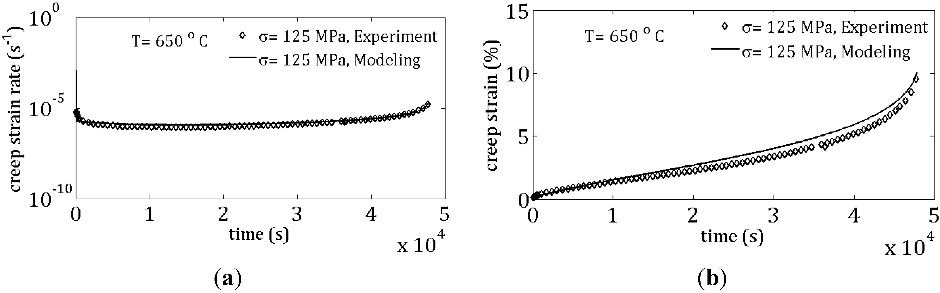
Metals 05 01487 g010
Figure 11. Creep results from experiments and finite element simulation for 125 MPa and 650 °C: (a) creep strain rate versus time; and (b) true creep strain versus time.
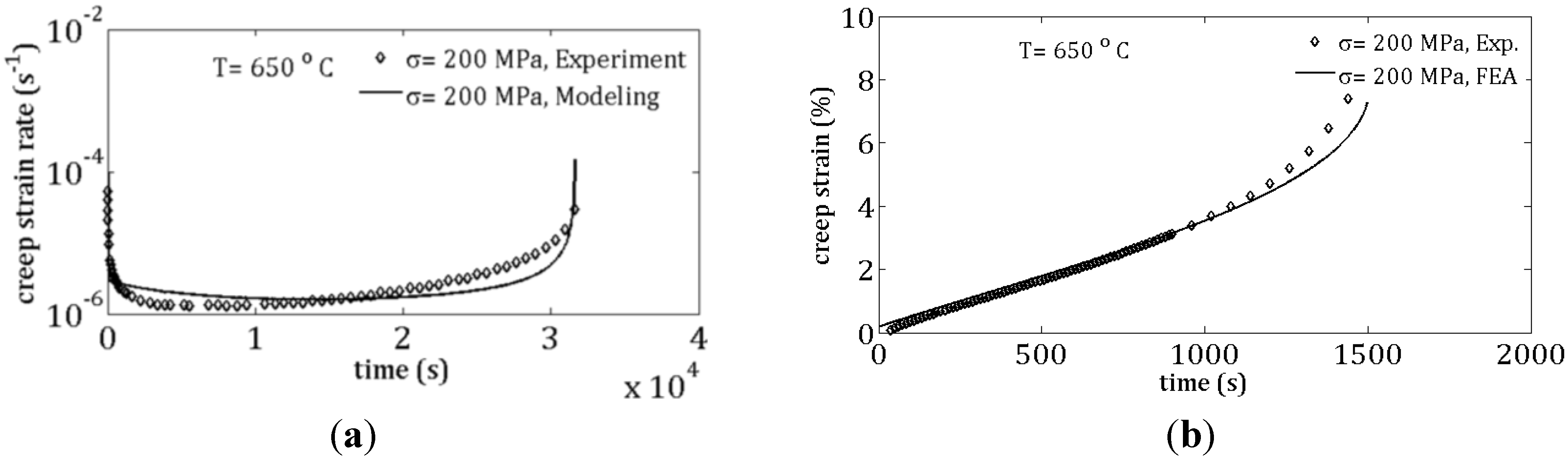
Metals 05 01487 g011
Figure 12. Creep results from experiments and finite element simulation for 200 MPa and 650 °C: (a) creep strain rate versus time; and (b) true creep strain versus time.
Metals 05 01487 g012
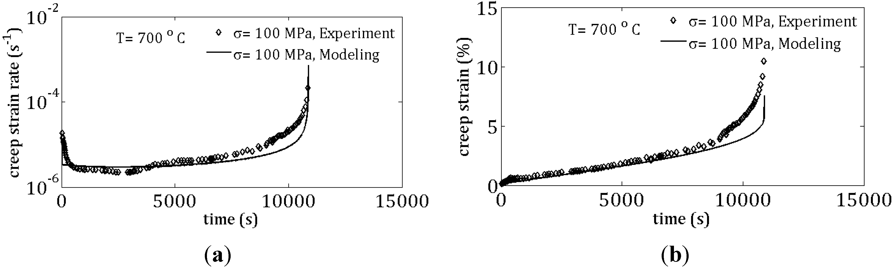
Figure 13a,b show the comparison of creep strain rate versus time and true creep strain versus time at 700 °C and applied stress of 100 MPa.
Figure 13. Creep results from experiments and finite element simulation for 100 MPa and 700 °C, (a) creep strain rate versus time; and (b) true creep strain versus time.
Metals 05 01487 g013
In general, the model predicts well the evolution of the total creep strain and the creep strain rate with time, as measured experimentally. This agreement is particularly true for the stage II creep in most of the loading conditions, while a slight disagreement between experimental and simulation data is recorded at the transition between successive stages of creep. The model under-predicts the accumulation of the creep strain with time for the 150 MPa and 600 °C, but this is mainly due to its inability to capture well the transition in the creep strain rate between the creep stage I and II. An overall assessment of the models leads to the conclusion that it can be used successfully to predict the deformation and fracture in modified 9Cr-1Mo welded steels for the large majority of testing conditions.
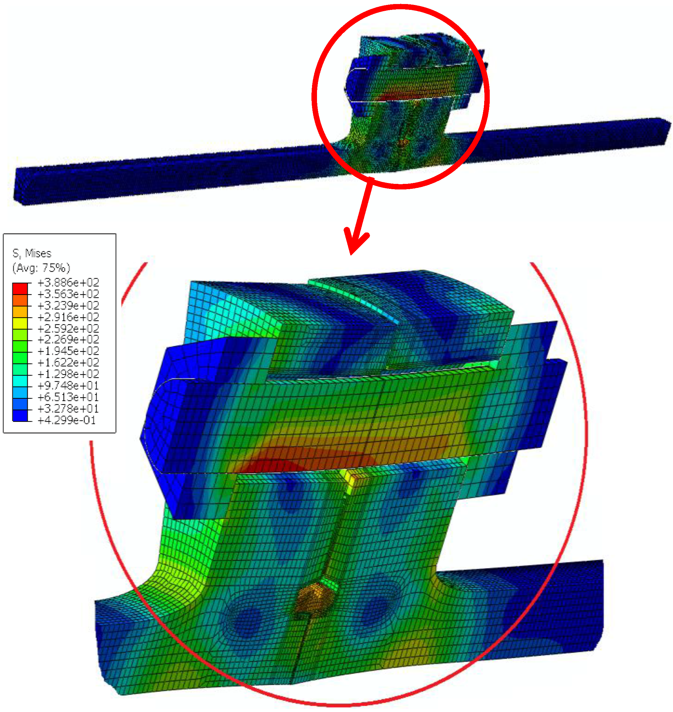
To exemplify the applicability of the constitutive model to three dimensional geometries, a creep simulation was performed for a pipe joined by a bolted connection to a flange. The pipe material was modified 9Cr-1Mo steel, while the flange material was Inconel X625. The operating temperature is 575 °C, and the internal pressure is 17 MPa. The bolt has been tightened down with a force equal to 7500 N and the simulation has been run for 100 h under these operating conditions. Due to symmetry, only a sector of the overall geometry was modeled in ABAQUS, and axisymmetric boundary conditions were used. As an illustration, the von Mises stress distribution developed after 100 h of creep in this bolted joint is plotted in Figure 14 on the deformed shape of the connection.
Figure 14. Example of a finite element simulation of creep stress distribution in a 9Cr-1Mo steel pipe connected to an Inconel X625 flange under thermo-mechanical loading. The operating temperature is 575 °C, and the internal pressure is 17 MPa.
Metals 05 01487 g014

6. Conclusions

A unified elasto-viscoplastic constitutive model for creep-damage was developed for modified 9Cr-1Mo welded steel. The model considered the main creep mechanism in this material to be the evolution of mobile dislocation density in the microstructure. In order to predict the stage III creep, several damage terms were introduced to capture the operating degradation phenomena in this steel. The model was implemented in ABAQUS using a User Material subroutine, and a semi-implicit numerical integration scheme was used to integrate the governing differential equations. Creep tests were conducted on welded and non-welded specimens made of modified 9Cr-1Mo steel. The creep tests were simulated in ABAQUS utilizing the developed numerical model. The modeling creep results show good correlations with the experimental results for the temperature range of 600–700 °C and stress range of 80 to 200 MPa. The model can be applied to study creep deformation and failure in three-dimensional complex geometries with different material properties.

Acknowledgments

The authors would like to gratefully acknowledge the Nuclear Energy University Program (NEUP) for providing the financial support for this research through DOE Grant 42246, release 59. Also, they would like to thank Sintra Co., Holland for sharing the ABAQUS input file for the three-dimensional flange connection. The author L.L.B.’s work was also supported by the National Science Foundation Major Research Instrumentation Program, grant 1229766.

Author Contributions

Mehdi Basirat has performed the model development, numerical implementation in ABAQUS and finite element simulations. Triratna Shrestha has performed the specimen preparation, experimental tests and microstructure analysis. Lyudmyla L. Barannyk has performed the numerical analysis on the material constants for the constitutive model. Gabriel P. Potirniche has provided guidance in the model development and simulations. Indrajit Charit has provided guidance in the experimental testing program.

Conflicts of Interest

The authors declare no conflict of interest.

References

  1. Shrestha, T.; Basirat, M.; Charit, I.; Potirniche, G.P.; Rink, K.K.; Sahaym, U. Creep deformation mechanisms in modified 9Cr-1Mo steel. J. Nucl. Mater. 2012, 423, 110–119. [Google Scholar] [CrossRef]
  2. Besson, J.; Leclercq, S.; Gaffard, V.; Gourgues-Lorenzon, A.-F. Analysis of creep lifetime of a ASME Grade 91 welded pipe. Eng. Fract. Mech. 2009, 76, 1460–1473. [Google Scholar] [CrossRef]
  3. Gaffard, V.; Gourgues-Lorenzon, A.F.; Besson, J. High temperature creep flow and damage properties of 9Cr1MoNbV steels: Base metal and weldment. Nucl. Eng. Des. 2005, 235, 2547–2562. [Google Scholar] [CrossRef]
  4. Yaghi, A.H.; Hyde, T.H.; Becker, A.; Sun, W. Finite element simulation of welding and residual stresses in a P91 steel pipe incorporating solid-state phase transformation and post-weld heat treatment. J. Strain Anal. Eng. Des. 2008, 43, 275–293. [Google Scholar] [CrossRef]
  5. Yaguchi, M.; Ogata, T.; Sakai, T. Creep strength of high chromium steels welded parts under multiaxial stress conditions. Int. J. Press. Vessels Pip. 2010, 87, 357–364. [Google Scholar] [CrossRef]
  6. Spigarelli, S.; Quadrini, E. Analysis of the creep behavior of modified P91 (9Cr-1Mo-NbV) welds. Mater. Des. 2002, 23, 547–552. [Google Scholar] [CrossRef]
  7. Hyde, T.H.; Tang, A. Creep analysis and life assessment using cross-weld specimens. Int. Mater. Rev. 1998, 43, 221–242. [Google Scholar] [CrossRef]
  8. Hyde, T.H.; Saber, M.; Sun, W. Creep crack growth data and prediction for a P91 weld at 650 °C. Int. J. Pressure Vessels Pip. 2010, 87, 721–729. [Google Scholar] [CrossRef]
  9. Auerkari, P.; Holmström, S.; Veivo, J.; Salonen, J. Creep damage and expected creep life for welded 9%–11% Cr steels. Proc. ECCC Creep Conf. 2007, 84, 69–74. [Google Scholar] [CrossRef]
  10. Watanabe, T.; Tabuchi, M.; Yamazaki, M.; Hongo, H.; Tanabe, T. Creep damage evaluation of 9Cr-1Mo-V-Nb steel welded joints showing Type IV fracture. Int. J. Pressure Vessels Pip. 2006, 83, 63–71. [Google Scholar] [CrossRef]
  11. Laha, K.; Chandravathi, K.S.; Parameswaran, P.; Sankara, R.K.B. Type IV Cracking Susceptibility in Weld Joints of Different Grades of Cr-Mo Ferritic Steel. Metall. Mater. Trans. A 2009, 40, 386–397. [Google Scholar] [CrossRef]
  12. Lee, H.-Y.; Kim, J.-B.; Kim, W.-G.; Lee, J.-H. Creep-fatigue crack behaviour of a modified 9Cr-1Mo steel structure with weldments. Trans. Indian Inst. Met. 2010, 63, 245–250. [Google Scholar] [CrossRef]
  13. Igari, T.; Fukahori, T.; Kawashima, F.; Tokiyoshi, T.; Chuman, Y.; Komai, N. Micro-macro creep damage simulation for welded joints. Mater. High Temp. 2011, 28, 181–187. [Google Scholar] [CrossRef]
  14. Basirat, M.; Shrestha, T.; Potirniche, G.P.; Charit, I.; Rink, K. A study of the creep behavior of modified 9Cr-1Mo steel using continuum-damage modeling. Int. J. Plast. 2012, 37, 95–107. [Google Scholar] [CrossRef]
  15. Weber, G.; Anand, L. Finite deformation constitutive equations and a time integrated procedure for isotropic hyperelastic and viscoplastic solids. Comput. Methods Appl. Mech. Eng. 1990, 79, 173–202. [Google Scholar] [CrossRef]
  16. Blum, W.; Eisenlohr, P.; Breutinger, F. Understanding creep—A review. Metall. Mater. Trans. A 2002, 33, 291–303. [Google Scholar] [CrossRef]
  17. Chilukuru, H.D.K. Coarsening of precipitates and degradation of creep resistance in tempered martensite steels. Mater. Sci. Eng. A 2009, 510–511, 81–87. [Google Scholar] [CrossRef]
  18. Morra, P.V.; Radelaar, S.; Yandouzi, M.; Chen, J.; Böttger, A.J. Precipitate coarsening-induced plasticity: Low temperature creep behaviour of tempered SAE 52100. Int. J. Plast. 2009, 25, 2331–2348. [Google Scholar] [CrossRef]
  19. Muñoz-Morris, M.A.; Gutierrez-Urrutia, I.; Morris, D.G. Influence of nanoprecipitates on the creep strength and ductility of a Fe–Ni–Al alloy. Int. J. Plast. 2009, 25, 1011–1023. [Google Scholar] [CrossRef]
  20. Lemaître, J. Mechanics of Solid Materials; Cambridge University Press: Cambridge, UK, 1990. [Google Scholar]
  21. Dunne, F. Introduction to Computational Plasticity; Oxford University Press: Oxford, UK; New York, NY, USA, 2007. [Google Scholar]
  22. Naumenko, K.D. Modeling of Creep for Structural Analysis; Springer: Berlin, Germany; New York, NY, USA, 2007. [Google Scholar]

