1. Introduction
Accurate prediction of the noise behaviour in metal walls is a challenging problem [
1]. The European Union’s Green Paper on Future Noise policy [
2] estimates 80 million people suffering from unacceptable noise levels that cause sleep disturbance and an additional 170 million having annoyance during the daytime due to inadequate acoustic insulation. The recent standard for buildings includes a requirement for increased acoustic resistance of light weight partition walls incorporating metal frames [
3].
The physics of noise behaviour and its interaction with structures have been extensively studied over the past years. This has helped to understand the noise behaviour of rooms and other enclosed spaces. Consequently, different measurement methods to quantify the noise behaviour of building materials have been standardized and used to generate data that are now available for building design [
3,
4]. However, these measurement techniques are often time-consuming and need highly specialized equipment. They also require differentiated setups along with expert technicians and can only be carried out in a specialist test laboratory.
The noise behaviour of metal-framed partition walls are currently recognized as one aspect of the total design criteria as can be seen from recent advances [
5]. Building standards are also being implemented, incorporating quantitative acoustical criteria, to ensure adequate noise isolation. Also, as multi-family housing using steel-framed partition walls become more common, designers are increasingly faced with the requirement of providing adequate sound insulation [
6]. Therefore, accurate and effective predictions of the noise behaviour of metal-framed walls are at the forefront of efficient building design.
The reasons for the higher noise transmission exhibited by metal-framed walls are due to the phenomenon of acoustic bridging [
1]. This has stimulated interest in efficient computational models that can simulate the acoustic insulation of common building elements, such as metal-framed walls. A typical measurement of noise behavior at one-third-octave bands consists of two independent reverberation chambers, which share a common interface. The metal-framed wall, whose noise behavior (sound reduction index,
R) to be measured, forms the common interface [
3,
4].
Significant research has been carried out in the field of analytical and numerical prediction of noise behavior [
7,
8,
9,
10,
11]. In most cases, simple plate-like structures were studied and analytical or semi-empirical formulas were derived [
12]. However, when these expressions were applied to common building structures, like metal-framed walls, the results did not compare well with experimental data. This is due to the geometrical criteria of transmission suites and standardized conditions of acoustic fields that lead to specific acoustic loading of the test specimen under fluid-structure interaction (FSI) [
13]. Moreover, predicting the airborne sound transmission through multilayer structures with cavities and structural links, under the influence of FSI, is a rather difficult task due to the complex dynamic system involved [
13,
14,
15,
16,
17].
Del coz Diaz
et al. [
16], in a recent study, mentioned that FE acoustic analysis using a 3D wall model is highly challenging because of the small mesh size required at high frequencies. This was found to be true, attempting to simulate a 3D model using traditional mesh methods; the solution time spanned across days. Consequently, it was deemed interesting to investigate the possibilities of using an efficient meshing procedure within a vibro-acoustic context. The lack of literature on FEM to predict the noise behaviour of building components has also been reported in various publications [
15,
16].
In this contribution, an efficient computational model to predict the noise behaviour of metal-framed walls at one-third-octaves is presented. The suitability of the model is evaluated with comparison to experimental test data following ISO 10140. The efficiency of the model is assessed by comparing the solution time between the traditional mesh methods and the proposed methods. A mesh sensitivity analysis along with the application of the proposed model to study the geometrical contribution of the stud sections towards the acoustic behaviour of metal-framed walls is also demonstrated.
2. Numerical Method
The vibrational noise of a wall produces acoustic pressure to the fluid with which it is in contact. Whatever the frequency of vibration, the resulting fluid pressure is governed by the acoustic wave equation [
18]. As the solid and fluid systems interact, a solution cannot be reached without considering the coupled system. Consequently, the fluid and the structural systems cannot be solved separately without considering the fluid-structure interaction (FSI) [
19]. For the current analysis, the fluid-structure interaction constitutes a sound field, which is influenced at a particular frequency by the properties of the air, geometry of the vibrating wall surfaces, types of fixing mechanism connecting the vibration surfaces, the material and damping properties at the interface, and the spatial distribution of the component of vibrational acceleration normal to the surface of the vibrating structures [
18,
19].
For the problem under consideration, the structural dynamics equation needs to be considered, along with Navier-Stokes equations and the flow continuity equation [
20]. The Navier-Stokes and continuity equations were simplified to get the acoustic wave equation, assuming the fluid is compressible, inviscid, constant flow rate, and the mean density and pressure are uniform throughout. Based on the assumptions listed below, the acoustic wave equation can be written as shown in Equation (1).
where,
is the sonic velocity and
is the acoustic pressure. Since the viscous dissipation has been neglected, Equation (1) can be considered as the lossless wave equation for propagation of sound in fluids. Accordingly, the harmonically varying pressure can be defined using Equation (2), where,
is the pressure amplitude and
is the angular velocity.
In order to completely describe the FSI, the fluid pressure loads acting at the interface should also be taken into account. When using the resulting dynamic elemental equation [
21] based on discretized acoustic wave equation most of the variables considered in this study can be represented. However, for the current analysis, additional terms and equations were also included, as discussed below, to reflect particular solutions and boundary conditions.
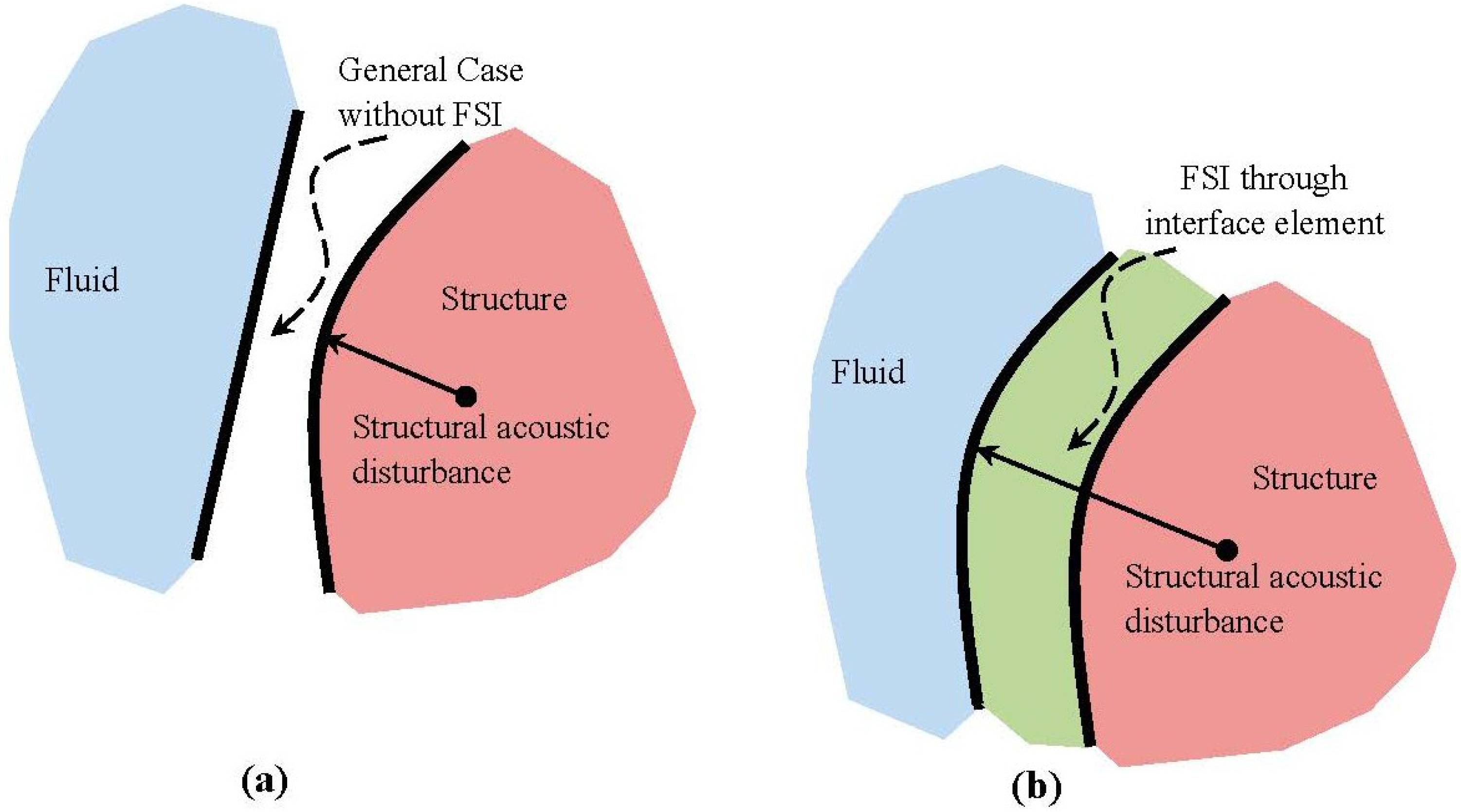
2.1. Fluid-Structure Interaction
The problem under consideration consists of two fluid-filled reverberation chambers coupled using a metal-framed wall, as shown in
Figure 1. The sound source in Room 1 produces pressure disturbances in the fluid with which it is in contact. This fluid disturbance induces a vibration on to Leaf 1 which is then transferred through the stud and air cavity on to Leaf 2. The vibration on Leaf 2 then induces a pressure disturbance to the fluid in Room 2 as shown in
Figure 2.
Figure 1.
Two fluid-filled reverberation chambers partitioned using a metal-framed wall.
Figure 2.
FSI between different components of the system considered; where s represents FSI between sound source and room air 1, a represents FSI between room air 1 and Leaf 1, b represents FSI between Leaf 2 and room air 2, c represents FSI between the stud and cavity air, and d represents FSI between cavity air and the two leaves.
When the structure and fluid systems interact, a solution cannot be obtained without considering the coupled system [
16,
17]. Accordingly, the simulation was executed using a real-time coupling between the structural and fluid elements accounting for FSI as shown in
Figure 3. Using this method, the structural properties can be modelled into their respective structural elements, fluid properties into the fluid elements, and interface properties (boundary admittance and FSI) into the interface elements.
ANSYS [
21] acoustic fluid elements, along with a 3D structural element, were used to model the system for the harmonic analysis. Acoustic Fluid30 elements were used to model the fluid part, along with Solid185 elements to build the structural part. The interfaces between the structural and fluid elements were modelled using Fluid30 with the element property algorithm option two set to zero [
21]. The air inside the room, which is not directly in contact with the structural elements, was modelled using a modified Fluid30 symmetric element with only pressure as a degree of freedom. This was highly beneficial in terms of computational time and storage, as the symmetric element matrices require less memory and can be executed efficiently.
Figure 3.
Coupling between the fluid and solid domains using an interface function; (a) decoupled structure and fluid elements; (b) coupled structure and fluid elements.
2.2. Geometrical Model
The geometric model consists of two reverberation chambers partitioned using an ISO 10140-compliant metal-framed wall with dimensions as shown in
Figure 1. The wall model consists of a 70 mm stud placed at 400 mm centre, sandwiched between two 15 mm gypsum plasterboards. The air cavity between the gypsum board and stud surfaces was also modelled to closely replicate the physical model. The lengths of the short and long flanges were 31 mm and 34 mm, respectively, with a material thickness of 0.5 mm.
The boundary walls of the reverberating chambers were considered rigid to prevent their contribution to the acoustic pressure due to structural vibration. However, the surface absorption was accommodated into the interface element at the fluid boundary. The sound source was modelled as a frequency-dependent, harmonically-varying displacement of 1 mm, with a dimension of 0.4 m × 0.8 m at the center of the source room wall. In order to avoid spurious effects, several excitation frequencies ranging from ±5% [
15] of the central frequencies at one-third-octave bands were considered.
2.3. Frequency Dependent Mesh
The noise behavior the metal-framed wall was analyzed over a frequency range of 100 Hz to 3150 Hz. A mesh sensitivity analysis was carried out from which it was found that the mesh dependency of the current problem can be represented using Equation (3), where is the sonic velocity, is the frequency, and is the maximum element length.
The common procedure for meshing an acoustic model is by using the element size corresponding to the highest frequency considered [
22]. Using a maximum frequency of 3150 Hz, the constant element size can be obtained as 0.014 m. However, using an element size of 0.014 m at one-third-octave bands increases the computational cost significantly. Consequently, a frequency dependent mesh closely following Equation (1) was adopted. In this way the smallest element size of 0.014 m was only required at a single iteration of 3150 Hz.
The frequency dependent mesh was modelled representing additional array parameters using FORTRAN commands within the Ansys Parametric Design Language (APDL). These arrays were then called in as meshing parameters referring to individual frequencies. In this way, the mesh is constantly modified throughout the simulation with respect to the frequency of iteration. The process continues in a loop until the final iteration, referring to a frequency of 3150 Hz, is reached.
2.4. Boundary Conditions
Different boundary conditions were specified to carry out the harmonic acoustic analysis and to recreate a realistic setting. The displacements at all external walls other than the metal-framed wall were constrained to zero. The top and bottom end of the stud were fixed in all directions. However, the stud flanges were allowed to vibrate freely and no fluid elements were constrained. In order to simplify the model and to provide a uniform mesh, the screw fixings between the stud and gypsum plasterboards were ignored and a continuous contact was specified.
Sound Wave Incidence
The method for simulating the diffuse field sound transmission was based on exciting the metal-framed wall through set of unrelated plane wave sources from the source room. The acoustic pressures generated through these excitations were then added to evaluate the incident acoustic pressure. An equivalent incident diffuse field was thus simulated through a set of plane waves applied on the wall boundaries in the source room. A feasibility study was conducted and found that a single wave was not able to represent diffuse field behaviour. However, a case of 12 plane waves, randomly distributed within the source room, were found to create an adequate diffuse field with a minimal impact on the solution time.
2.5. Post Processing
Using the finite element acoustic fluid pressure, the sound pressure level (L) was calculated using Equation (4); where is the root mean square pressure and defaults to 20 × 10−6 Pa. Once the sound pressure level within the source and receiving rooms is computed, Equation (5) was used to evaluate the sound reduction index (R) of the wall with an area (S) and equivalent absorption area (A).
2.6. Material Properties
The air inside the room for the analysis was represented using an acoustic fluid element with density and sonic velocity as material properties. Additionally, the frequency-dependent boundary admittance (μ) was specified for the fluid elements in contact with the structural components to accommodate absorption along the structural surfaces. For structural elements, Young’s modulus, density, Poisson’s ratio, and damping were specified as listed in
Table 1.
Table 1.
Material Properties.
| Material | E (Pa) | ρ (kg/m3) | ν | c (m/s) |
|---|
| Steel | | 7929 | 0.31 | - |
| Gypsum | | 1000 | 0.25 | - |
| Mortar | | 2000 | 0.17 | - |
| Air | - | 1.25 | - | 338 |
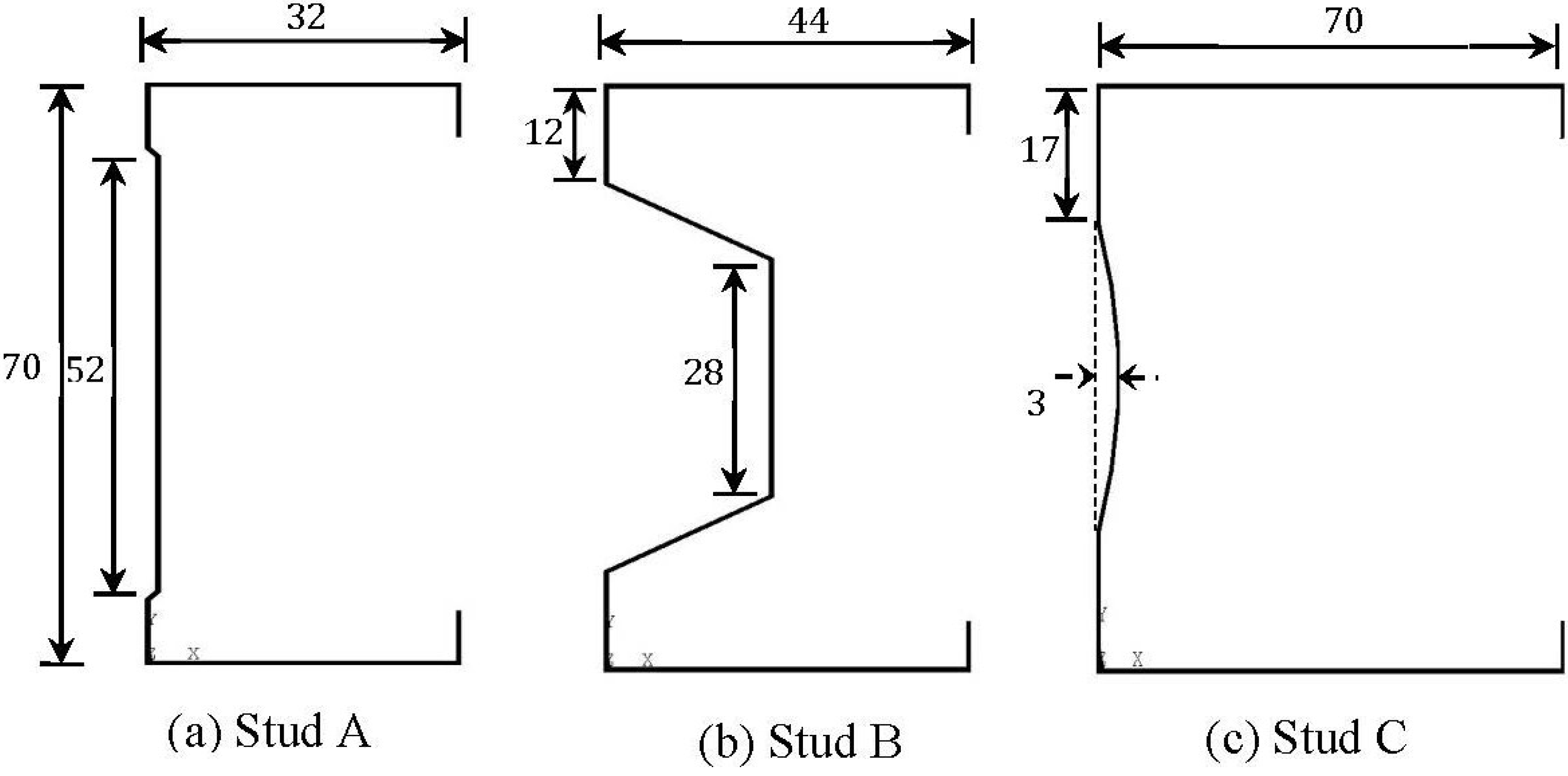
2.7. Stud Geometries
It was interesting to analyse the sound reduction index using FEA for the partition wall using various stud geometries to evaluate the possibility of using FEA to predict the acoustic insulation of partition walls with respect to small variations in stud geometries. The study was significant as it could aid in the development of improved stud designs for acoustic efficiency. Consequently, acoustic analyses of metal-framed walls with three different stud geometries designed by Hadley Industries were performed. The stud geometries were designated A, B, and C with section geometries as shown in
Figure 4.
Figure 4.
Schematic of the stud sections analyzed (all dimensions in mm).
3. Experimental Test
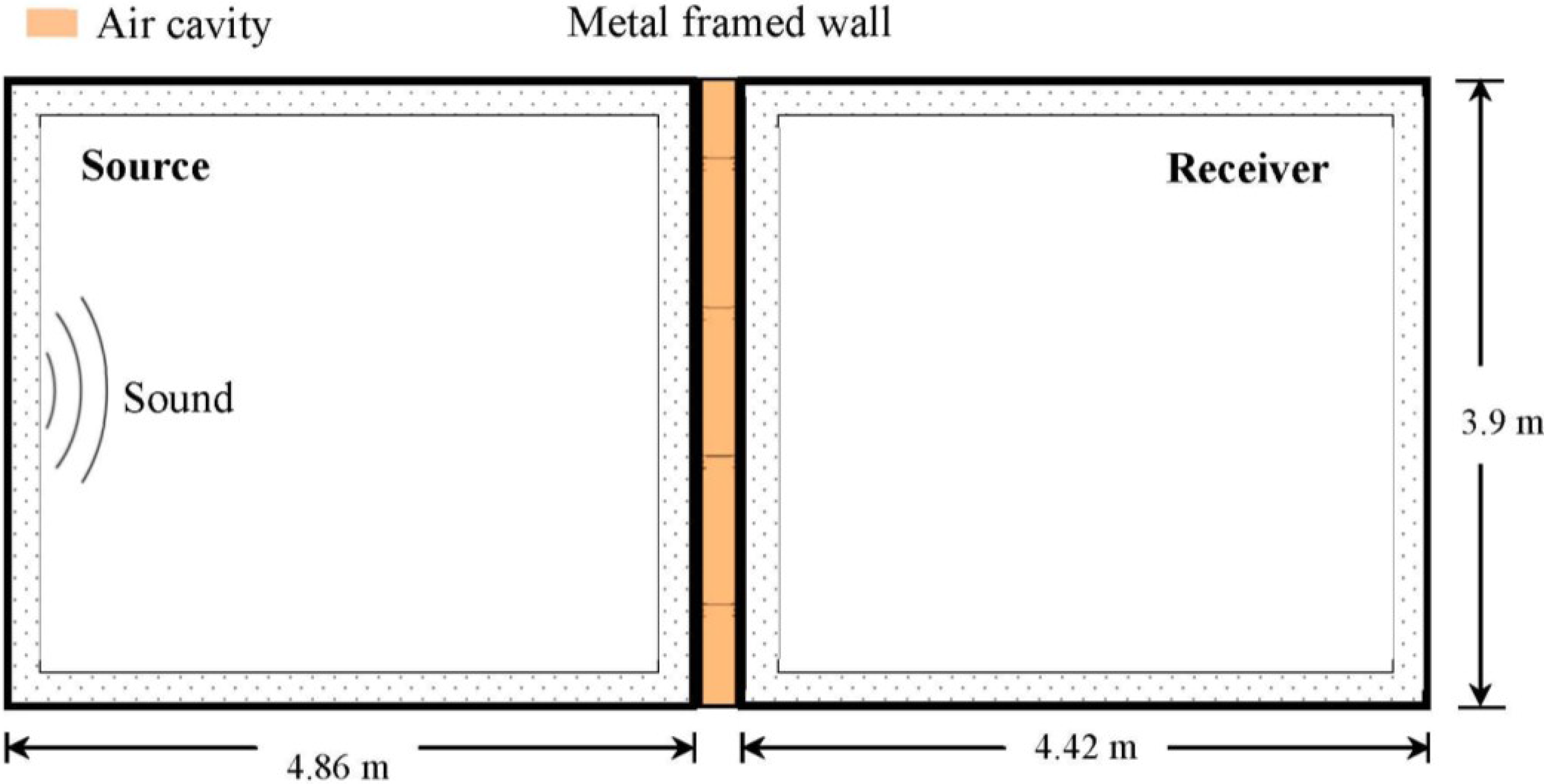
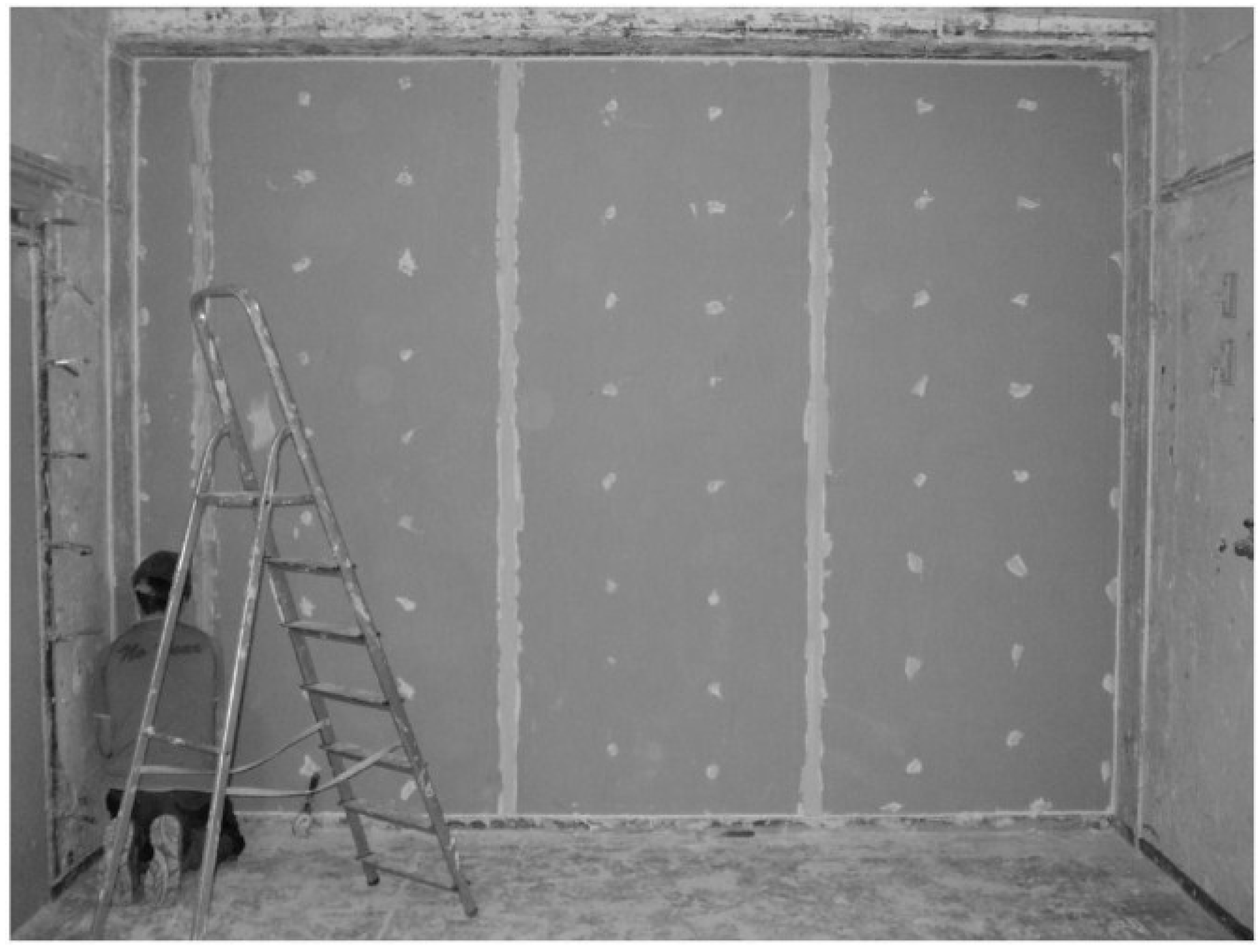
A partition wall made up of 11 steel studs was tested within a plasterboard partition. The tests were conducted at the Sound Research Laboratories (SRL) (Suffolk, UK) using BS/ISO standards and UKAS-accredited best practice procedures. The tests were conducted at an average air humidity of 61% and 31%.
The partition construction was one layer of 15 mm dense acoustic plasterboard on either side of the stud. The studs were placed at 400 mm centres in the perimeter channel which spanned the top and bottom of the aperture. Plasterboards were screwed to the studs at 300 mm centres and the joints were taped. The perimeter of the partition was sealed with mastic on both sides, as shown in
Figure 5. The partition measured 3.85 m in width and 2.92 m height.
Figure 5.
Mastic sealing on the metal-framed wall perimeter for the experimental test.
The samples were mounted, positioned, and tested in accordance with ISO 10140 [
4]. The measurement uncertainty for sound reduction index at one-third-octave band frequency, according to the British standards, is listed in
Table 2. The values of uncertainty were based on a standard uncertainty multiplied by a coverage factor of
k = 2, which provides a level of confidence of approximately 95%. The evaluation of uncertainty in the experimental measurement of sound reduction index are detailed in ISO 10140.
Table 2.
Experimental test measurement uncertainty.
| Frequency, Hz | Uncertainty, ±dB |
|---|
| 100 | 2.6 |
| 125 | 2.4 |
| 160 | 2.1 |
| 200 | 2.1 |
| 250 | 1.5 |
| 315 | 1.5 |
| 400 | 1.2 |
| 500 | 1.2 |
| 800–3150 | 1.0 |
The airborne sound transmission was determined from the difference in sound pressure levels measured across the test sample installed between two reverberant rooms. The difference in measured sound pressure levels is corrected for the amount of absorption in the receiving room. The test is done under conditions which restrict the transmission of sound by paths other than directly through the sample, and the sound field was made to be randomly incident on the sample.
The test sample partitions the two rectangular reverberant acoustically live rooms; both of which were constructed from 215 mm brick with mortar plastering and reinforced concrete floors and roofs. The brick wall has dimensions of 3.9 m (width) × 2.9 m (height) and forms the whole of the common area between the two rooms.
One of the rooms, termed the source room (Room 1), has a volume of 55 cubic meters and is isolated by the use of resilient mountings and seals, from the surrounding structure and the adjoining room. The adjoining receiving room (Room 2) has a volume of 50 cubic meters.
Broadband noise is produced in the source room (Room 1) from an electronic generator, power amplifier, and loudspeaker. The resulting sound pressure levels in both rooms were sampled, filtered into one-third-octave band widths, integrated, and averaged by means of a real time analyser using a microphone on an oscillating microphone boom. The value obtained at any particular frequency is known as the equivalent sound pressure level for either source or receiving rooms. The change in level across the test sample is termed the equivalent sound pressure level difference.
4. Results and Discussion
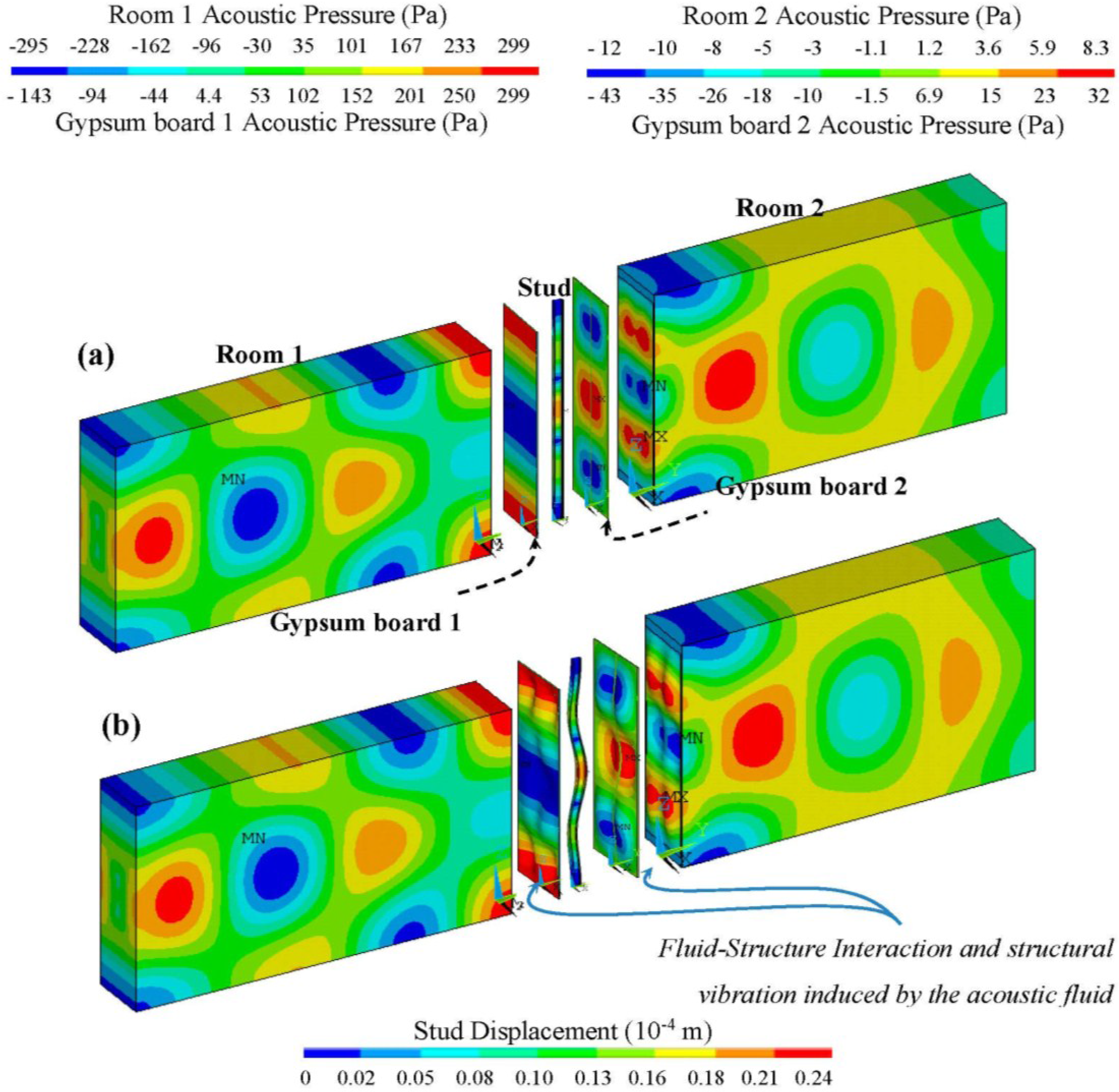
The pressure distribution within the room-wall-room model for a frequency of 160 Hz is shown in
Figure 6a. The effective coupling between the acoustic-fluid and structure due to FSI can be related to the pressure distribution shown. The acoustically-induced vibration of the stud and gypsum board during sound transmission is also visualised (
Figure 6b). This shows that the FE procedure presented is effective in modelling FSI and acoustic-fluid structure coupling to simulate a realistic scenario. However, it should be noted that spatial acoustic pressure distribution is not constant within the source and receiving room and it varies with the difference in the boundary conditions of the metal-framed wall dividing the two rooms.
For example, the acoustic pressure at the longitudinal centre of the wall is different from the boundaries of the wall where the motion is constrained due to the boundary of the reverberation chambers. A single span section of the numerical model as opposed to the 11 stud model at a frequency of 160 Hz is presented to visualise the fluid-structure interaction. However, the equivalent sound levels were evaluated by averaging the nodal pressure within the reverberation rooms taking into account spatial acoustic distribution in all the three dimensions. Compared to the experimental test, the FEA allows the visualisation of the acoustic pressure distribution. However, further studies are needed to derive optimisation algorithms that can be used for the geometric optimisation to the walls and rooms for better acoustic performances.
Figure 6.
Pressure distribution for a frequency of 160 Hz, showing FSI, (a) true scale view and (b) scaled displacement view with a magnification factor of 2000 showing acoustically-induced structural vibration.
Using the coupled model, the sound reduction index at one-third-octave bands for a range of constant mesh sizes (0.014 to 0.40 m) were analysed (
Figure 7). This was done to study the mesh sensitivity in calculating the
R values with respect to frequency. The maximum and minimum mesh sizes were selected using Equation (1) for a frequency of 3150 Hz (0.014 m) and 100 Hz (0.40 m).
In comparing the
R values as shown in
Figure 7, it can be seen that the mesh size has a significant effect on the
R values obtained. The impact of mesh size was found to be maximum at high frequencies and minimum at low frequencies. The highest differences in
R values for all the frequencies were exhibited for a mesh size of 0.40 m followed by 0.20 m. Even though these mesh sizes comply with Equation (3) for a frequency range of 100 Hz to 200 Hz, the
R values obtained at these frequencies were poor compared to the other mesh sizes tested.
Figure 7.
Comparison of Sound Reduction Index at one-third-octave bands for various mesh sizes, (a) 0.014–0.050 m and (b) 0.10–0.40 m.
When the R values for a mesh size of 0.1 m for a frequency range of 100 Hz to 400 Hz were compared to lower mesh sizes of 0.050 m, 0.025 m and 0.014 m, an average difference of only 1.69 dB was observed with a lowest difference of 0.24 dB at 100 Hz and 3.8 dB at 250 Hz. Accordingly, for a frequency range of 100 Hz to 400 Hz a mesh size of 0.1 m can yield satisfactory results at a significantly lower computational cost compared to a mesh size of 0.014 m.
Comparing further the R values, it was found that the best results for a frequency range of 500–800 Hz, 1000–1600 Hz and 2000–3150 Hz were observed at mesh sizes of 0.05 m, 0.025 m, and 0.014 m, respectively. This shows that the frequency range of 500 Hz to 3150 Hz comply with Equation (1) for best possible results with minimal solution time.
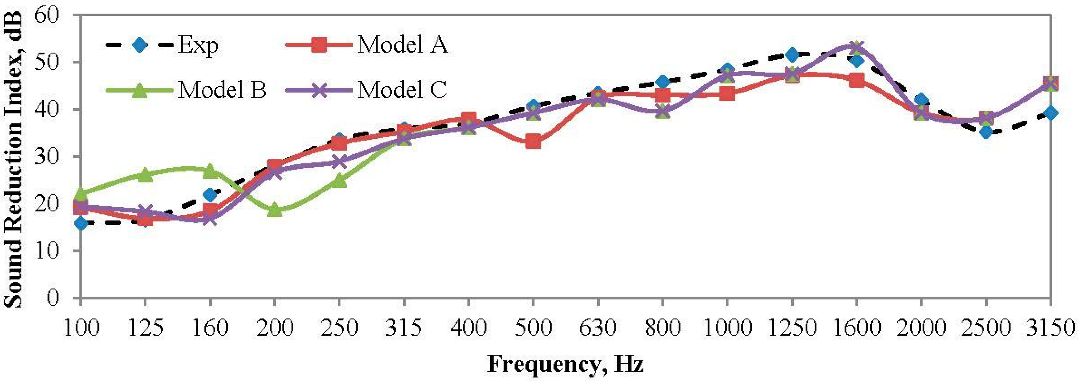
Following this trend from the mesh sensitivity analysis, a frequency-dependent mesh model was developed. The element sizes used for this model (Model C) relating to the frequency of excitation is as listed in
Table 3. Model A shows the element size used for the constant mesh model and Model B shows the mesh size complying with Equation (3).
Table 3.
Element size distribution with respect to frequency at one-third-octave bands.
| Frequency (Hz) | Model A (m) | Model B (m) | Model C (m) |
|---|
| 100 | 0.014 | 0.430 | 0.10 |
| 125 | 0.014 | 0.340 | 0.10 |
| 160 | 0.014 | 0.270 | 0.10 |
| 200 | 0.014 | 0.210 | 0.10 |
| 250 | 0.014 | 0.170 | 0.10 |
| 315 | 0.014 | 0.140 | 0.10 |
| 400 | 0.014 | 0.110 | 0.10 |
| 500 | 0.014 | 0.086 | 0.086 |
| 630 | 0.014 | 0.068 | 0.068 |
| 800 | 0.014 | 0.054 | 0.054 |
| 1000 | 0.014 | 0.043 | 0.043 |
| 1250 | 0.014 | 0.034 | 0.034 |
| 1600 | 0.014 | 0.027 | 0.027 |
| 2000 | 0.014 | 0.021 | 0.021 |
| 2500 | 0.014 | 0.017 | 0.017 |
| 3150 | 0.014 | 0.014 | 0.014 |
Comparing the results as shown in
Figure 8, Model B exhibits minimal convergence of the three at low frequencies. This shows that the mesh size predicted using Equation (3) does not satisfy the minimum element length requirement at low frequencies. The best results were exhibited by Model A (constant mesh) and Model C (optimised, frequency-dependent mesh). However, the solution time for Model A was found to be significantly higher than that of Model C.
Figure 8.
Comparison of Sound Reduction Index between the constant and frequency dependent mesh models considered.
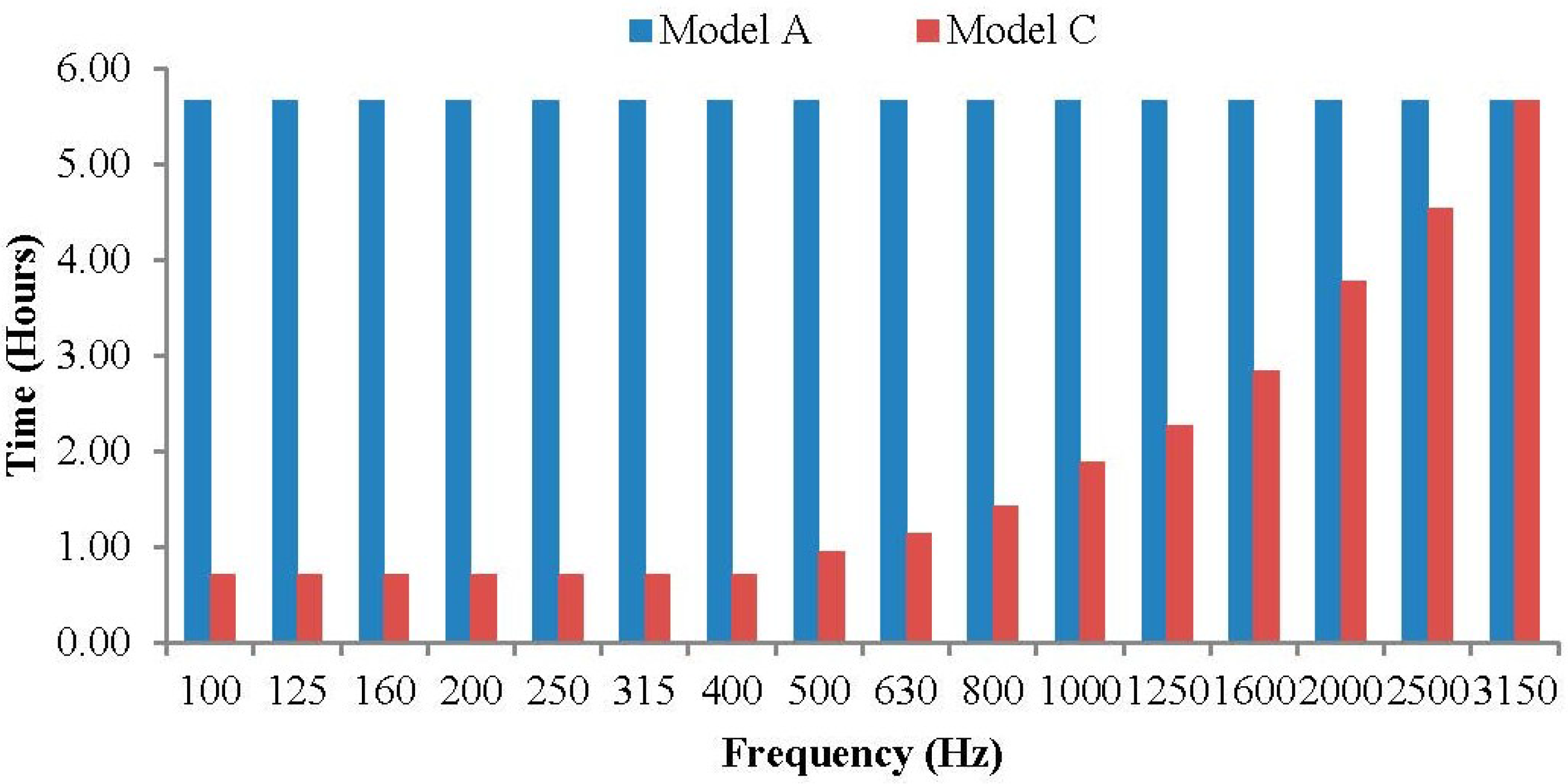
The solution times for Model A and Model C are shown in
Figure 9. It was observed that a better solution time for almost all the frequencies except 3150 Hz were obtained using the frequency-dependent mesh model developed. When the overall solution time was compared, Model A took 91 h and Model C took 29:30 h to complete 16 iterations. This was an improvement in the solution time of 60:30 h using the new model proposed.
Figure 9.
Comparison in solution time between the constant mesh (Model A) and frequency dependent mesh (Model C) at one-third-octave bands.
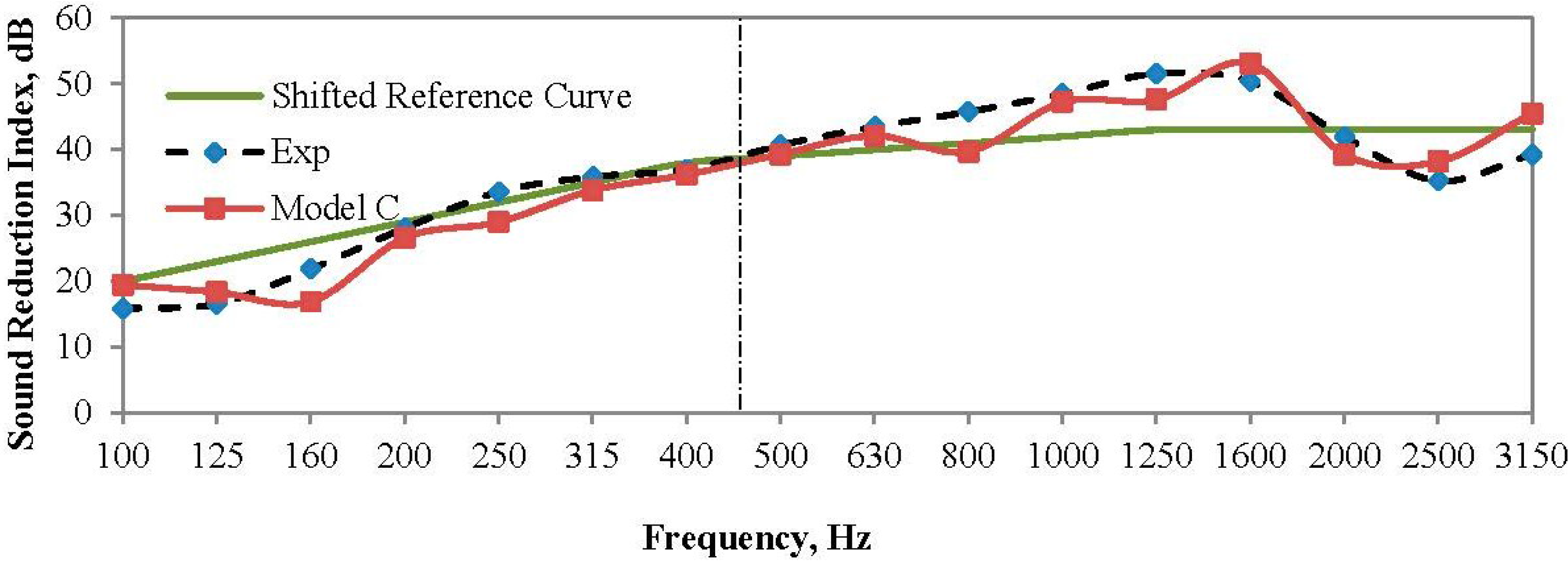
Based on the measured R values, the single-number quantity representing the acoustic insulation commonly known as Rw(C; Ctr) is calculated, where, C represents the acoustic insulation of the wall constituting sound produced from living activities, high- and medium-speed train noise, motorways (speed > 80 km/h), and factories with high- and medium-frequency noise. Ctr represents performance under urban road traffic, low-speed train noise, and factories with low- and medium-frequency noise.
The Rw(C; Ctr) for Model A and Model C were calculated to be 39(−3; −7) and 38(−2; −7), respectively. Comparing the values with the experimental result of 39(−2; −7) Model C was found to be in good agreement with the experimental data with only a variation of 1 dB.
Even though the
R values used to compute
Rw(
C;
Ctr) exhibited differences of 5 dB, 4.6 dB, 6.1 dB, and 6.2 dB at 160 Hz, 250 Hz, 800 Hz, and 3150 Hz respectively, it was interesting to see that the
Rw(
C;
Ctr) values only differed by 1 dB. This was due to the standardised reference curve [
4] used for the calculation. From
Figure 10, it can be seen that the shifted reference curve at 500 Hz based on FEA lies closely with the experimental data, giving an
Rw(
C;
Ctr) value close to the experimental data.
Figure 10.
Shifted reference curve with respect to measured R values.
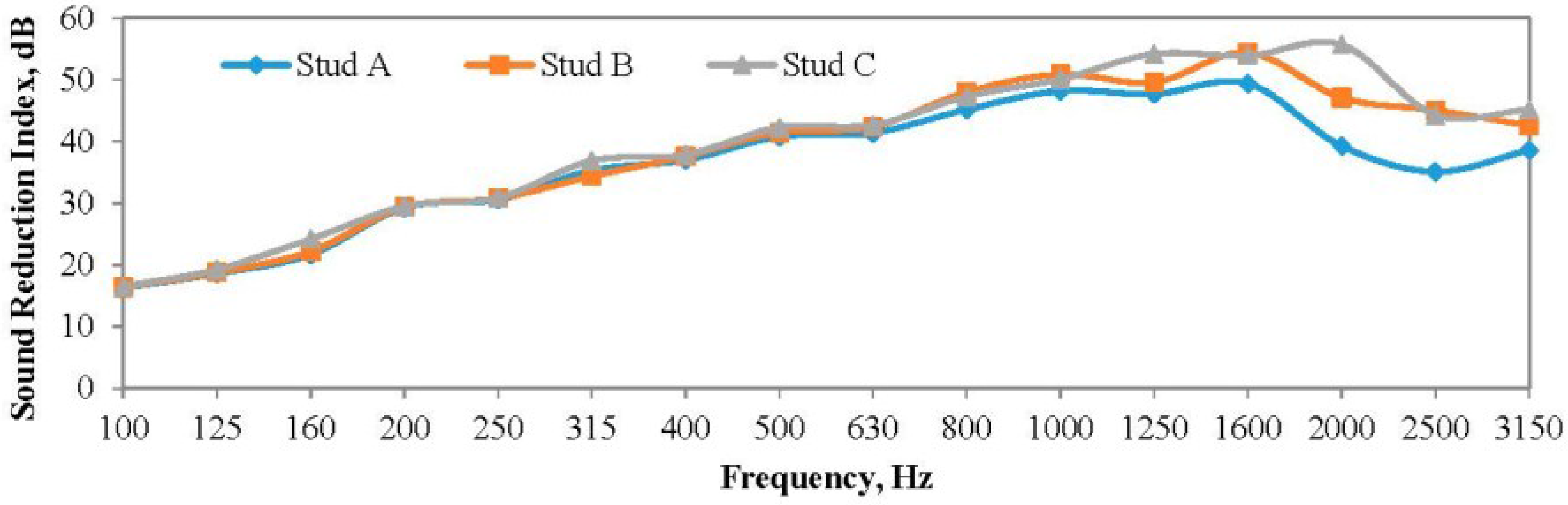
The
R values of the partition wall using stud geometries A, B, and C are shown in
Figure 11. Comparing the results, it can be observed that the geometry of the stud has an effect on the overall acoustic insulation of the metal-framed wall.
Figure 11.
R values from experimental test for a metal-framed wall using various stud geometries.
Average differences in the Sound Reduction Index of 4 dB were observed between a frequency range of 100 Hz to 400 Hz, when Stud B and Stud C were compared to Stud A. The difference in the values was highest at 160 Hz, with 8 dB between Stud A–Stud B and Stud A–Stud C. However, this difference was reduced to 1.3 dB at 400 Hz.
For the frequency range of 500–3150 Hz, an average difference in the R values of 3 dB was exhibited between walls using Stud A–Stud B and 3.5 dB between Stud A–Stud C. The wall with Stud C exhibits the highest sound reduction index for most of the frequencies tested, followed by the sound reduction performance of wall with Stud B. The lowest sound reduction performance was exhibited by the wall using Stud A.
The Rw(C; Ctr) for walls using Stud A, Stud B, and Stud C were 40(−3; −8), 42(−3; −11), and 43(−2; −8), respectively. The results show that the wall using Stud C exhibits the highest acoustic insulation, with Stud B and Stud A following. Even though the trend exhibited by the Rw(C; Ctr) values were similar to the R values, the differences exhibited by the single-number quantity were found to be small (2 dB) when compared to the differences between the frequency dependent R values (8 dB) between the geometries tested.
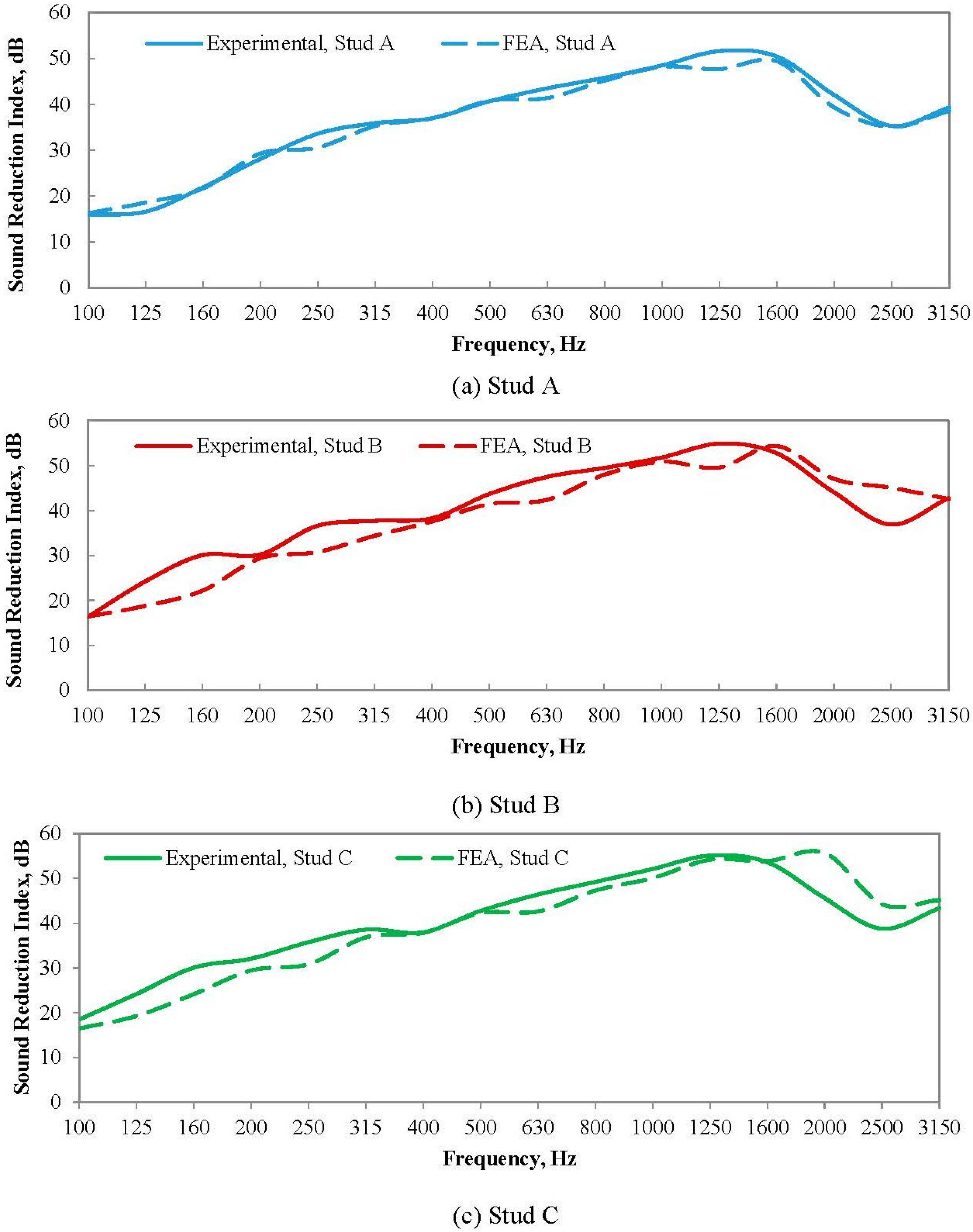
The
R values for the metal-framed wall using three different stud geometries obtained using FEA are shown in
Figure 12. The results predicted Stud C to have the best acoustic insulation, with Stud B and Stud A following; a trend similar to the experimental results. However, the FEA results showed only average differences of 1 dB at low frequencies (100–500 Hz) between the three stud geometries. This was a difference of 3 dB, compared to the experimental test results. The reason for this may be the simplified contact between the stud and the gypsum board, along with the variation in the connection technique used. For the experimental test, the gypsum board and the studs were held together using a screw-fixed setup, but for the FEA a continuous contact between the stud and the gypsum board were assumed to simplify the model.
Figure 12.
R values using FEA for a metal-framed wall using various stud geometries.
The
Rw(
C;
Ctr) calculated using the FEA results for the wall with Stud A, Stud B, and Stud C were 40(−2; −8), 41(−3; −8), and 42(−3; −9), respectively. Comparing the
Rw(
C;
Ctr) calculated using FEA and experimental results, an average difference of only ±1 dB was observed. This ±1 dB difference in the weighted sound reduction index was due to the variations in the frequency-dependent
R values between the FEA and experimental results as shown in
Figure 13. The ±1 dB difference between the two methods cannot be used to evaluate the accuracy of the FEA model, as it masks the substantial difference exhibited by the
R values at certain frequencies. Therefore, a comparison of the
R values at one-third-octave band is considered to evaluate the accuracy of the FE model developed.
Figure 13.
Comparison of R values using FEA and experimental tests for (a) Stud A; (b) Stud B; and (c) Stud C.
The comparison of the frequency dependent
R values between the experimental test and FEA are shown in
Figure 13. The dotted lines represent the FEA and the continuous lines represent the experimental results. Comparing the results, it can be observed that both FEA and experimental tests show similar trends in the sound reduction index. However, a certain difference in the actual values obtained between the two methods was observed.
The variations in the results were highest with 3.9 dB for Stud A, 8.2 dB for Stud B, and 9.1 dB for Stud C at 1250 Hz, 2500 Hz, and 2000 Hz, respectively. The higher variations in the frequency dependent R values between the two methods for Stud B and Stud C were due to the mean average method used for calculating the sound reduction index.
In order to account for resonance due to the wall’s natural frequency, and to avoid spurious effects, the sound reduction index for the wall was plotted for several frequencies within ±5% of the central frequencies, and the mean average of the values was taken to obtain the best possible results for FEA. This technique was proposed by Del Coz Díaz
et al. [
16] in their work to predict the acoustic behaviour of masonry walls using FEA.
Based on the results obtained, it is proposed that the FE modelling and meshing procedure presented in this work can be used to efficiently simulate a 3D room-wall-room model and to predict the sound reduction index of metal-framed walls. The proposed method can also be extended to study the acoustic behaviour of other building components undergoing FSI at a lower computational cost. It is also suggested that FE software packages facilitate a non-uniform frequency-dependent mesh matrix allowing users to vary the mesh sizes as a component of frequency to perform large acoustic simulations in an efficient manner.
The preliminary study on the application of the numerical model suggests that improved sound reduction performance can be obtained for steel-framed walls by modifying the stud geometries. However, in order develop optimum stud geometry, design guidelines relating to the acoustic performance need to be put forward based on extensive analysis.
This study is limited to stud walls with no absorbing material in the air cavity between the studs. However, it is anticipated that the effect of stud geometry can be magnified by minimizing the sound transmission through the air cavity. Therefore it would be interesting to conduct further research on the acoustic simulation of stud walls with porous sound absorbing in-fill materials. This is also an area that currently lacks literature in the FE research community. It is also acknowledged that the experimental comparison in this study is used for validation of the numerical model and not for error estimation. Consequently, detailed error estimation studies will be required to identify strategies to further improve the accuracy of the numerical model.


