The Promising Features of New Nano Liquid Metals—Liquid Sodium Containing Titanium Nanoparticles (LSnanop)

Abstract

A new kind of suspension liquid was developed by dispersing Ti nanoparticles (10 nm) in liquid Na, which was then determined by TEM (transmission electron microscopy) analysis. The volume fraction was estimated to be 0.0088 from the analyzed Ti concentration (2 at. %) and the densities of Ti and Na. This suspension liquid, Liquid Sodium containing nanoparticles of titanium (LSnanop), shows, despite only a small addition of Ti nanoparticles, many striking features, namely a negative deviation of 3.9% from the ideal solution for the atomic volume, an increase of 17% in surface tension, a decrease of 11% for the reaction heat to water, and the suppression of chemical reactivity to water and oxygen. The decrease in reaction heat to water seems to be derived from the existence of excess cohesive energy of LSnanop. The excess cohesive energy was discussed based on simple theoretical analyses, with particular emphasis on the screening effect. The suppression of reactivity is discussed with the relation to the decrease of heat of reaction to water or the excess cohesive energy, surface tension, the action as a plug of Ti oxide, negative adsorption on the surface of LSnanop, and percolation.

1. Introduction

The study of liquid metals has been an interesting fundamental field of physics [1,2,3] since Ziman [4] developed the electron transport theory of liquid metals, in which the Born approximation of electron scattering theory was coupled with the pseudopotential theory. On the other hand, this has also been an important subject in material science and for industrial technologies, such as refining and casting of metals and steels. Furthermore, in the fast reactor technology, liquid Na, a typical example of liquid metals, is an indispensable material for realizing excellent heat exchange. However, as is well known, liquid Na sometimes reacts with water and oxygen explosively, with large heat generation. This high reactivity of liquid Na causes difficult problems if present, such as severe accidents, for which some countermeasures must be prepared beforehand. It is very important to suppress the chemical reactivity of liquid Na to water and oxygen.

Recently, liquids containing nanoparticles (nanometer size) have attracted considerable attention with the goal of obtaining excellent thermal conductors [5]. This kind of liquid has been called a “nanofluid”. The motivation of these fluids is derived from the idea that the poor thermal conductivity of a fluid (or liquid) medium is supplemented by the high thermal conductivity of the suspended nanoparticles. Recent advances in so-called nanotechnology has made the stability of this kind of suspension liquid very rigorous; that is, the sedimentation problem of suspended particles in this kind of liquid might be removed by the adoption of particles of nanometer size instead of millimeter or micrometer size. However, the expectations for this kind of suspension liquid are not limited to only the improvement of thermal conductivity. In fact, development has been made for ferrofluids or magnetic fluids of organic liquid medium, whose fluid behavior can be controlled easily by a magnetic field. In this case, fine particles are coated with lyophilic organic molecules of long C (carbon)–C (carbon) bond chain, by which, together with the avoidance of particle agglomeration, an improvement in wettability is achieved between the fine particles and the organic medium. Even magnetic fluids with liquid metal medium have been reported in several cases [6,7,8], though such a surface coating is not always realized in the metallic medium.

In principle, it is possible to provide many interesting and valuable properties to this kind of suspension liquid through the combination of different nanoparticle and liquid medium materials. Liquid Na is an important thermal medium for fast reactor technology because of its high thermal conductivity. The largest problem to overcome is the danger caused by the high reactivity of liquid Na to oxygen and water. This chemical reactivity of liquid Na is desired to be removed by the introduction of nanoparticles into liquid Na. In fact, Ara and coworkers [9,10,11,12,13,14] succeeded in suppressing the chemical reactivity of liquid Na by introducing Ti nanoparticles. Kim et al. [15] performed theoretical analysis of the stability of this liquid Na containing Ti nanoparticles. In this article, the preparation, physicochemical properties, and stability of liquid Na containing Ti nanoparticles are reviewed, from the fundamental point of view, based on the studies of Ara and coworkers [9,10,11,12,13,14], particularly Saito et al. [13]. Hereafter, liquid Na containing Ti nanoparticles is referred to as “LSnanop” (Liquid Sodium containing nanoparticles of titanium).

2. The Design of LSnanop

The suppression of liquid Na’s chemical reactivity might be realized by introducing, as nanoparticles, elements that are more reactive than Na. The Ellingham diagram, or the standard Gibbs free energy of oxide formation as a function of temperature [16], tells us that this is possible, at least for the suppression of reactivity to oxygen, by the introduction of Ti, Cr, Mn, V, Si, and/or Al into liquid Na, whose standard Gibbs free energy of oxide formation is lower than that of Na. Noting the importance of bonding energy to the stability of nanoparticles in liquid Na, Saito and Ara [12] performed the preliminary density functional calculation of small size clusters composed of Na atoms and 3d- and 4d-transition element atoms; the bond energy and the charge transfer from Na atoms to nanoparticles were systematically analyzed. Ara and coworkers conclusively selected Ti among them.

The next problem is the stability of the suspension liquids. Under the absence of mutual solubility, it is not always easy to keep particles in the suspended state in a liquid medium stable by preventing sedimentation or floating problems. Therefore, the Brownian motion of suspended particles must be considered in detail. We consider the situation that a spherical Ti nanoparticle with radius r_N is dropped into liquid Na, whose density and viscosity are ρ_Na and η_Na, respectively. The suspension of nanoparticles in liquid Na can be realized by the mechanism of Brownian motion; that is, the kinetic energy of dropping nanoparticles with the terminal velocity U does not exceed the thermal energy, (1/2)k_BT (k_B: the Boltzmann’s constant; T: the absolute temperature), of Na atoms in liquid Na. The upper limit of radius, or the critical radius, r_N^C for the permanent itinerant motion, is given as follows [17]:

$${r_N}^C={\left\{\frac{243}{16\pi }\frac{C^2{{\text{η}}_{\text{Na}}}^2{k}_{B}T}{{\text{ρ}}_{\text{Na}}{({\text{ρ}}_{\text{Nano}}-{\text{ρ}}_{\text{Na}})}^2{g}^2}\right\}}^{1/7}$$

(1)

In Equation (1), ρ_Nano represents the density of nanoparticle and g is the gravitational acceleration. C indicates the boundary condition dependence of Stokes’ law, F_r = 6πr_NUC, for the friction force, Fr, against a falling sphere (radius r_N) of velocity U; C = 1 for the stick boundary condition and C = 2/3 for the slip boundary one [18]. In the case of macroscopic spherical particles, the stick boundary condition has been conventionally employed for the derivation of terminal velocity. However, it is known that, in the microscopic case, there is the possibility that the slip boundary condition works well for Stokes’ law, as is shown in the model liquid composed of hard spheres [19]. In addition, since the wettability of Ti to liquid Na is not good, both cases were considered in Equation (1) [13].

The r_N^C in Equation (1) was obtained for the simple case in which the tendency of aggregation of nanoparticles due to, for example, the magnetic interactions, was left out of consideration. Therefore, by following the implication of Goto [17], the safety critical radius, r_N^sc, is introduced as r_N^sc = fr_N^C; the value of f can be taken to be less than 1 to alleviate the danger of sedimentation due to the agglomeration of nanoparticles by the additional inter-particle interaction. Goto [17] implied that the value of f might be near 1/100 if magnetic interactions exist. In the case of LSnanop, Ti nanoparticles do not seem to be ferromagnetic, judging from a simple preliminary experiment in which the LSnanop was not attracted by a rare earth magnet (Nd₂Fe₁₄B). Therefore, the value of f = 1/100 should be far to the safe side.

Figure 1 shows the safety critical radii, r_N^sc’s, for three cases, f = 1, f = 1/10 and f = 1/100, of LSnanop as a function of temperature. The dependence of boundary condition for Stokes’ law on the critical radii is also shown in this figure by open circles for the slip boundary (A) and solid circles for the stick boundary condition (B). The difference of boundary condition is not so significant. Ara and coworkers [9,10,11,12,13,14] introduced Ti nanoparticles of 10 nm diameter into liquid Na (LSnanop).

Figure 1. Temperature dependence of safety critical radius, r_N^sc, for titanium nanoparticles in liquid Na; open circle: slip boundary condition (A); and solid circle: stick boundary condition (B).

Figure 1. Temperature dependence of safety critical radius, r_N^sc, for titanium nanoparticles in liquid Na; open circle: slip boundary condition (A); and solid circle: stick boundary condition (B).

As can be seen in Figure 1, Ti nanoparticles of 10 nm diameter can be safely suspended in liquid Na, even if the inter-particle interaction is strong (f = 1/100), like in magnetic fluids. In addition, the LSnanop with nanoparticles of 10 nm diameter is kept stable, even in higher temperature ranges, such as 800 K. In the case of magnetic liquids with organic solvent medium, magnetic particles are coated with lyophilic organic molecules of long C–C bond chain, which keeps the inter-particle distance longer. This prevents the mutual collision and aggregation of particles in addition to increasing the lyophilic property. The adoption of such a technique is difficult in the case of LSnanop. Therefore, it is essential for the stability of LSnanop to introduce fine particles of nanometer size into liquid Na. As seen in Figure 1, Ti nanoparticles with up to a 20 nm radius may stabilize the LSnanop.

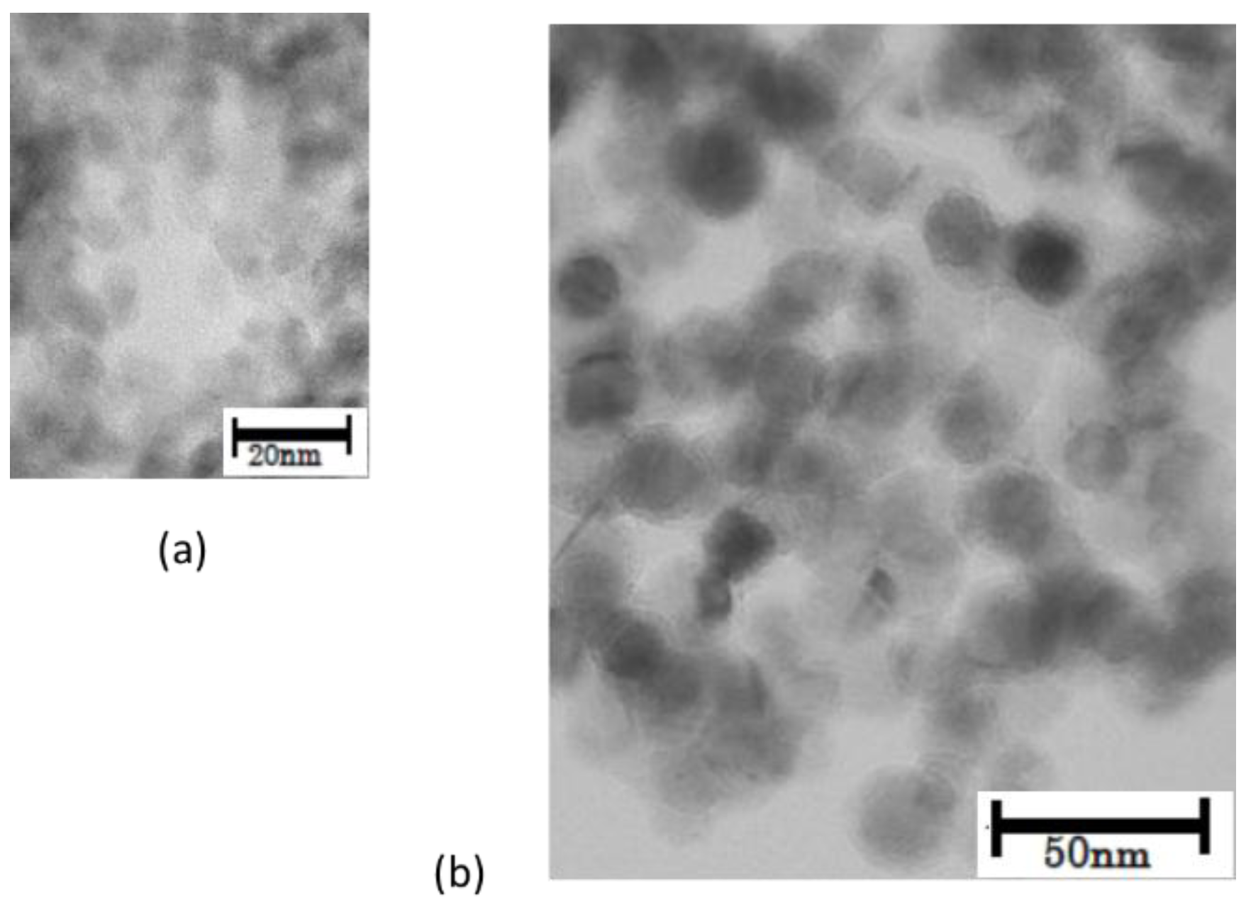
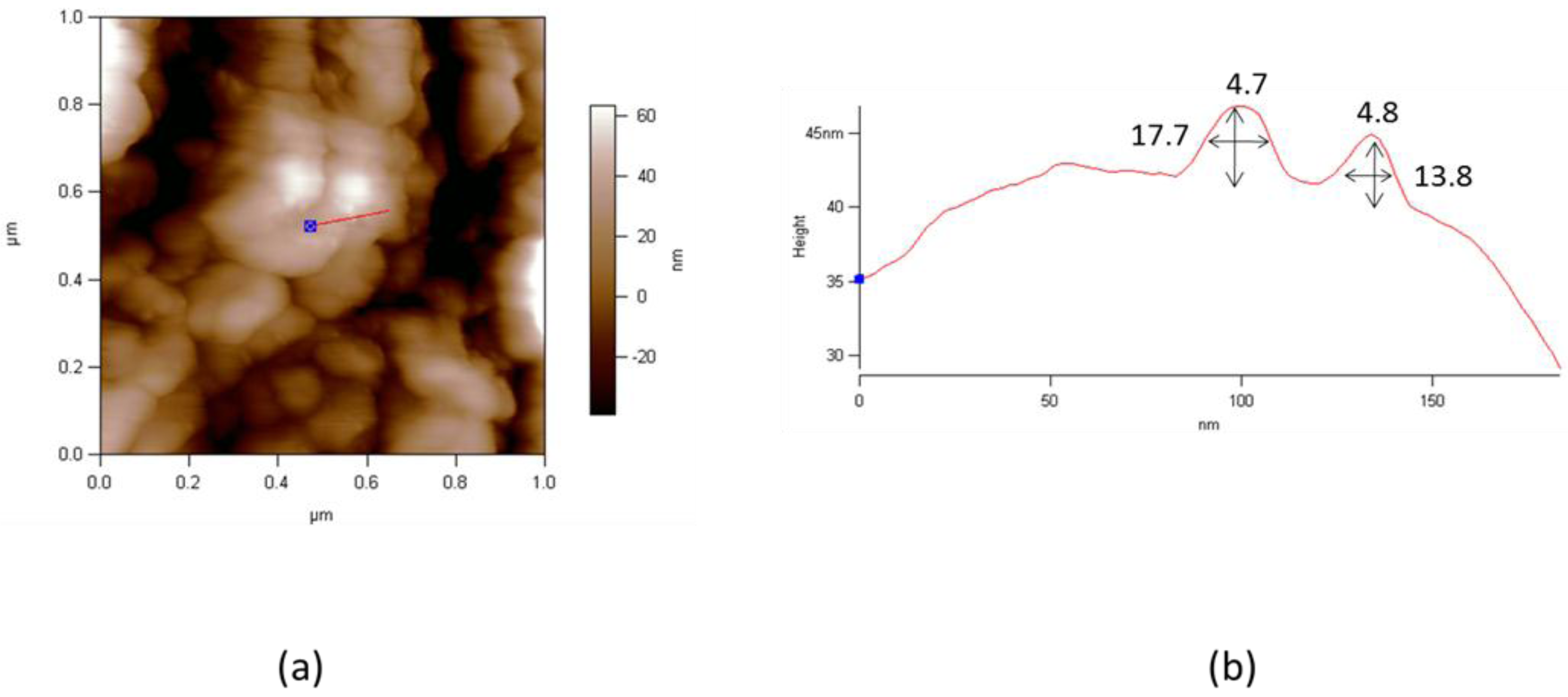
3. Preparation and Characterization of LSnanop

The electrodeposition technique has been adopted for the preparation of magnetic fluids with liquid Hg medium [6,7,8]; the electrolysis of electrolyte solution was applied to the introduction of ferromagnetic Fe and Co nanoparticles into liquid Hg. However, in the case of LSnanop, such a direct technique is not always valid due to the chemical reactivity of liquid Na to the electrolyte solution. Therefore, at present, the LSnanop must be prepared by the combination of two processes: nanoparticle preparation, followed by their introduction into liquid Na.

The Ti nanoparticles were prepared by the vapor deposition method in vacuum [20]. Prepared nanoparticles were always handled in an atmosphere of high purity argon gas (99.9999%). The surface of the prepared nanoparticles was kept clean under the condition of no oxidation. The average diameter of Ti nanoparticles, as determined by TEM (transmission electron microscopy) analysis on a Cu mesh, was approximately 10 nm [13]. The nanoparticles were dispersed into liquid Na at 623 K by using a stirrer and with the addition of ultrasonic sound waves, which were required because of the rather poor wettability of Ti nanoparticles to liquid Na in addition to their tendency to gather. Na metal of high purity grade (4.1 ppm O) was employed. Ti nanoparticles and Na metal were handled in a glove box with the circulation of high purity Ar gas (99.9999%). The concentrations of both oxygen and moisture in the glove box were kept below 0.1 ppm. The concentration of Ti in the obtained LSnanop was analyzed by the ICP-AES (inductively coupled plasma-atomic emission spectrometry). The reason it was necessary to perform concentration determination by ICP-AES is that during the preparation process it was not always easy to retain all the Ti nanoparticles in the LSnanop. The concentration of Ti in the LSnanop supplied to the experiments was found to be 2 at. %; namely, the number fraction (“atomic fraction”) of Ti is 2 atomic % as the binary mixture between Ti atoms and Na ones. The number fraction and the volume fraction of nanoparticles are estimated to be 6.92 × 10⁻⁷ and 0.0088, respectively, as described in Section 4.

The dispersed state of nanoparticles was investigated in the solid state using both TEM and AFM (atomic force microscopy). In principle, the observation in the liquid state may be desired. However, both observations were performed for the solidified samples due to the experimental difficulty of observation in the liquid state. To avoid the reaction of the sample to both oxygen and moisture, the preparation of samples for both observations was performed in the glove box described above. The handling for both techniques was done in high purity Ar gas atmosphere (99.9999%). During the TEM observation, the sample was always cooled with the use of liquid N₂ to avoid evaporation of Na due to the temperature increase on the electron beam irradiation. Figure 2 shows the dispersed state of Ti nanoparticles in the solidified LSnanop. As can be seen in this figure, Ti nanoparticles are not present in the clustered state, but in the independent particle state.

Figure 2. (a,b) TEM images of solidified LSnanop.

Figure 2. (a,b) TEM images of solidified LSnanop.

The cross sectional area of the solidified sample of LSnanop was also investigated using AFM [13]. The phase imaging of noncontact AFM clearly showed Ti nanoparticles as the hard part and Na as the soft part. In addition, the unevenness of the surface was detected using geometrical imaging. Such imaging photographs clearly show that the ~10 nm Ti nanoparticles are dispersed in the LSnanop [13]. Figure 3a shows the superposition of geometrical imaging and phase one for one cross section of the LSnanop. In Figure 3b, the distribution of unevenness in some part (along the red line from the blue spot in Figure 3a) is also shown. As can be seen in this figure, the small convex parts of 5 nm diameter are dispersed on the surface. This also indicates that Ti nanoparticles of nanometer size are dispersed in the LSnanop, though the size of nanoparticles is somewhat arbitrary, depending on the cutting surface and the observation spot.

Figure 3. AFM photograph of a cross section of the solidified LSnanop, (a) superposition of geometrical imaging and phase one; and (b) height distribution along the red line from the blue spot in (a).

Figure 3. AFM photograph of a cross section of the solidified LSnanop, (a) superposition of geometrical imaging and phase one; and (b) height distribution along the red line from the blue spot in (a).

4. Fundamental View Point of LSnanop

As described in Section 3, we already have information about the LSnanop, such as the Ti atomic fraction (2 at. %), the shape (spherical) and the size of Ti nanoparticles (10 nm diameter). Therefore, it is very important to grasp the fundamental view point of LSnanop for the discussion of the physicochemical properties and excess cohesive energy . For liquid Na, the system is considered to be composed of one mole of Na (total atoms, via Avogadro’s number, N_A (6.022 × 10²³)). Similarly, the system considered for the LSnanop contains Na atoms of Avogadro’s number, N_A, and Ti atoms of 2 at. % ((1/49) N_A), as 10 nm diameter nanoparticles. For simplicity, the radius of Ti nanoparticles, r_N, is assumed to be 5 nm only, which is almost supported by the direct observation of nanoparticles by TEM [13]. Then, the number of Ti atoms in one Ti nanoparticle, n_Ti, is estimated to be 2.95 × 10⁴ (2.99 × 10⁴) by assuming the density data of Ti metal [21]. The value of n_Ti is slightly dependent on the input data values, such as temperature and data sources. For example, in the present review, the estimation is performed at 500 K instead of 473 K, which was adopted in the previous paper [13]. Therefore, a slightly different value from the previous paper [13] was estimated in this review. The previously estimated values in Ref. [13] are written in parentheses in this section. The number of Ti nanoparticles, N_Nano, is 4.17 × 10¹⁷ (4.11 × 10¹⁷). The volume fraction of Ti nanoparticles is 0.0088 (0.007). The number fraction of Ti nanoparticles, X_Nano, is 6.92 × 10⁻⁷ (6.83 × 10⁻⁷); namely, the LSnanop is an extremely dilute mixture of Ti nanoparticles. We can define the nanoparticle spheres, whose radius, R_N, is defined as V_M^LSnanop = (4π/3)R_N³N_Nano; V_M^LSnanop is the volume of LSnanop containing Na atoms of the Avogadro’s number, N_A, and Ti atoms of 2 at. %. The value of R_N for the LSnanop is 24.2 (24.6) nm. On average, Na atoms can be considered to exist between two concentric spheres of radii R_N and r_N. This spherical shell, with the thickness of 19.2 (19.6) nm (R_N-r_N), contains 1.473 × 10⁶ (1.465 × 10⁶) Na atoms. This thickness, 19.2 (19.6) nm, is far larger than the correlation length of the liquid structure in liquid Na, which can be estimated from the distance of disappearance of oscillatory behavior on the radial distribution function, about 1 nm [22]. The system of LSnanop seems to still be a considerably large system for molecular simulations, such as ab initio molecular dynamics.

5. Physicochemical Properties of LSnanop

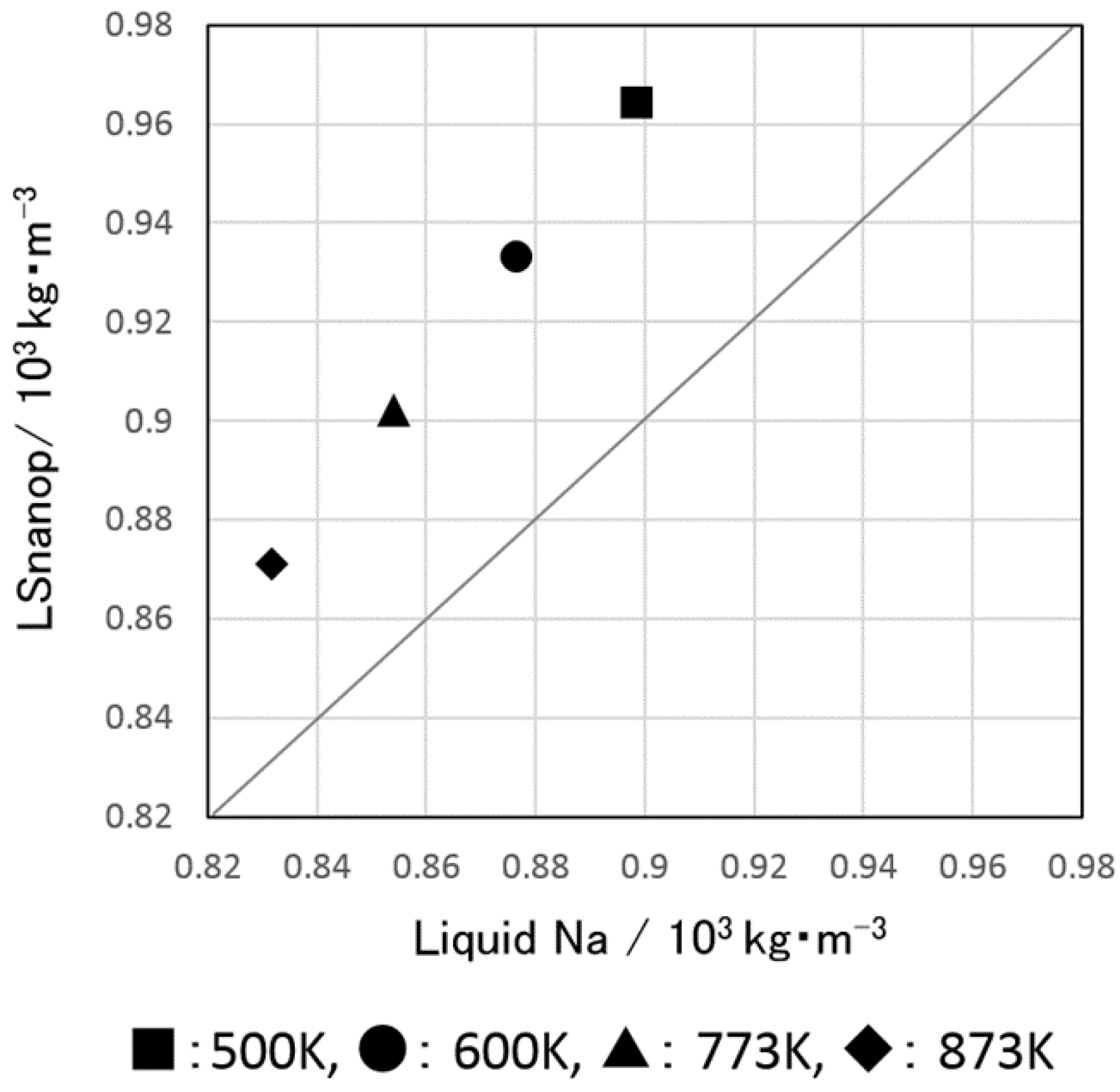
5.1. Density and Atomic Volume of LSnanop

In Ref. [13], the density, d (/10³ kg·m⁻³), for the LSnanop and liquid Na was given as a linear function of absolute temperature, T (/K), as d = aT + b in the temperature range from 473 to 773 K. The given coefficients are, a = −3.11 × 10⁻⁴ and b = 1.12 for the LSnanop and a = −2.23 × 10⁻⁴ and b = 1.01 for liquid Na [13]. The density of liquid Na given in Ref. [13] is in excellent agreement with the literature data [23]. This indicates the reliability of measured values of density and the adopted experimental method, the drop image method [13]. Figure 4 shows the comparison of density between the LSnanop and liquid Na in the temperature range from 500 to 873 K. The density of LSnanop is about 4.8% larger than that of liquid Na, as can be seen from the plotted data points, which are situated on the upper region from the slanted line.

Figure 4. Comparison of the densities of LSnanop and liquid Na: The slanted line corresponds to the hypothetical case in which the densities of the LSnanop and liquid Na are the same.

Figure 4. Comparison of the densities of LSnanop and liquid Na: The slanted line corresponds to the hypothetical case in which the densities of the LSnanop and liquid Na are the same.

Similarly, the atomic volume, V_M (/10⁻⁶ m³·mol⁻¹), which is related to the density as M/d (M: atomic mass), is expressed as a linear function of T as V_M = a’T + b’. The coefficients determined in this review are a’ = 0.0087 and b’ = 19.987 for the LSnanop and a’ = 0.0069 and b’ = 22.141 for liquid Na. From the density of LSnanop, the atomic volume of LSnanop is estimated to be about 4.9% smaller than that of liquid Na. It should be noted that this V_M for the LSnanop is evaluated as a hypothetical system, with 2 at. % Ti of a binary Na atom–Ti atom system whose total number of atoms is the Avogadro’s number (system A). However, in principle, the LSnanop should be considered a system composed of Na atoms and Ti nanoparticles (system B) whose number fraction of Ti nanoparticles, X_Nano, is 6.92 × 10⁻⁷, as described in Section 4. Therefore, from this fundamental point of view, the LSnanop is a very dilute system of Ti nanoparticles.

The atomic volume of LSnanop shows a negative deviation of 3.9% from the ideal solution (linear law) [13], which is drawn as a function of at. % Ti between the atomic volume of liquid Na and that of Ti metal at 500 K (system A). If the density of Ti nanoparticles is assumed to be same as that of bulk Ti metal [21], a slightly larger negative deviation of 5.7% from the ideal solution (linear law) can be obtained for system B, a binary mixture of Na atom and Ti nanoparticle. With the addition of an extremely small number of Ti nanoparticles (X_Nano = 6.92 × 10⁻⁷), the LSnanop shows a striking shrinkage of 5.7% from the ideal solution. This striking result implies the existence of excess cohesive energy for the LSnanop, which is discussed later in this review.

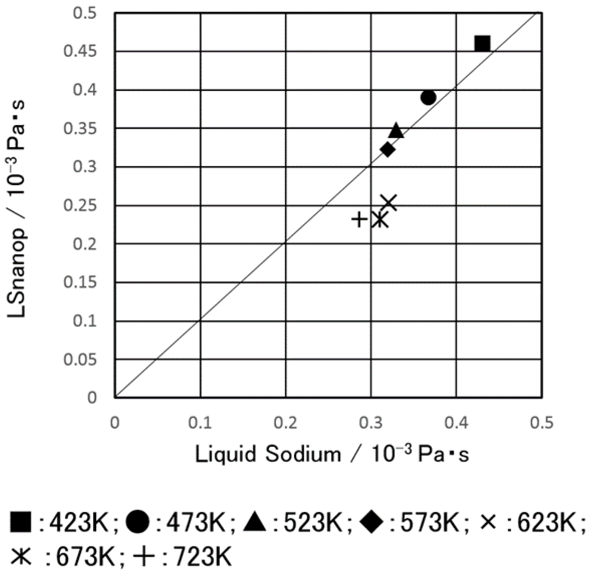
5.2. Shear Viscosity of LSnanop

In Figure 5 a comparison of shear viscosity between the LSnanop and liquid Na in the temperature range from 423 to 723 K is shown [13]. As can be seen in this figure, in the low temperature range, the data of shear viscosity for the LSnanop is situated slightly on the upper region, namely the shear viscosity of LSnanop is slightly larger than that of liquid Na. However, in the high temperature range, the shear viscosity of LSnanop is lower than that of liquid Na. The shear viscosity of liquid Na itself [13] is comparable to the literature [24]. It should be remembered that, at least partially, this difference seems to be derived from the experimental limitation. In the case of the rotational vibration method adopted for the measurements [13], the range of measurements is officially from 10⁻⁵ to 10⁻² Pa·s and the experimental error range was ±0.25 × 10⁻⁴~±0.38 × 10⁻⁴ Pa·s. Therefore, in the previous paper [13], the shear viscosity of LSnanop was concluded to be almost the same as that of liquid Na within the experimental error range. The measured data of shear viscosity should be considered only for the comparison between LSnanop and liquid Na. Anyways, the difference is very small and the shear viscosity of LSnanop may be almost the same as that of liquid Na.

Figure 5. Comparison of the shear viscosities of LSnanop and liquid Na: The slanted line corresponds to the hypothetical case in which the viscosities of LSnanop and liquid Na are equal.

Figure 5. Comparison of the shear viscosities of LSnanop and liquid Na: The slanted line corresponds to the hypothetical case in which the viscosities of LSnanop and liquid Na are equal.

From the theoretical point of view, the shear viscosity of suspension liquid can be considered by the so-called Einstein’s formula [25,26],

$$\text{η}={\text{η}}_0\left(1+2.5\varphi \right)$$

(2)

In Equation (2), η and η₀ are, respectively, the viscosity of suspension liquid and that of medium liquid; ϕ is the volume fraction of suspended particles. The volume fraction can be estimated to be 0.0088, as described in Section 4. By inserting this volume fraction into Equation (2), the obtained viscosity is η = 1.022η₀; namely, only a 2.2% increase in viscosity is predicted by Equation (2). As already described in Section 4, the estimation of volume fraction has some ambiguities and it was assumed to be 0.007 in the previous paper [13]. Therefore, the calculated result for η in the present review is slightly different from the previous prediction, η = 1.020η₀ [13], though the difference itself is not so significant. The prediction due to the Einstein’s relation is slightly contradictory to the experimental data in the high temperature range; namely, the experimental shear viscosity of LSnanop is slightly smaller than that of liquid Na, as shown in Figure 5. Therefore, from the fundamental point of view, whether Einstein’s relation is valid or not for the LSnanop should be experimentally and theoretically studied in detail.

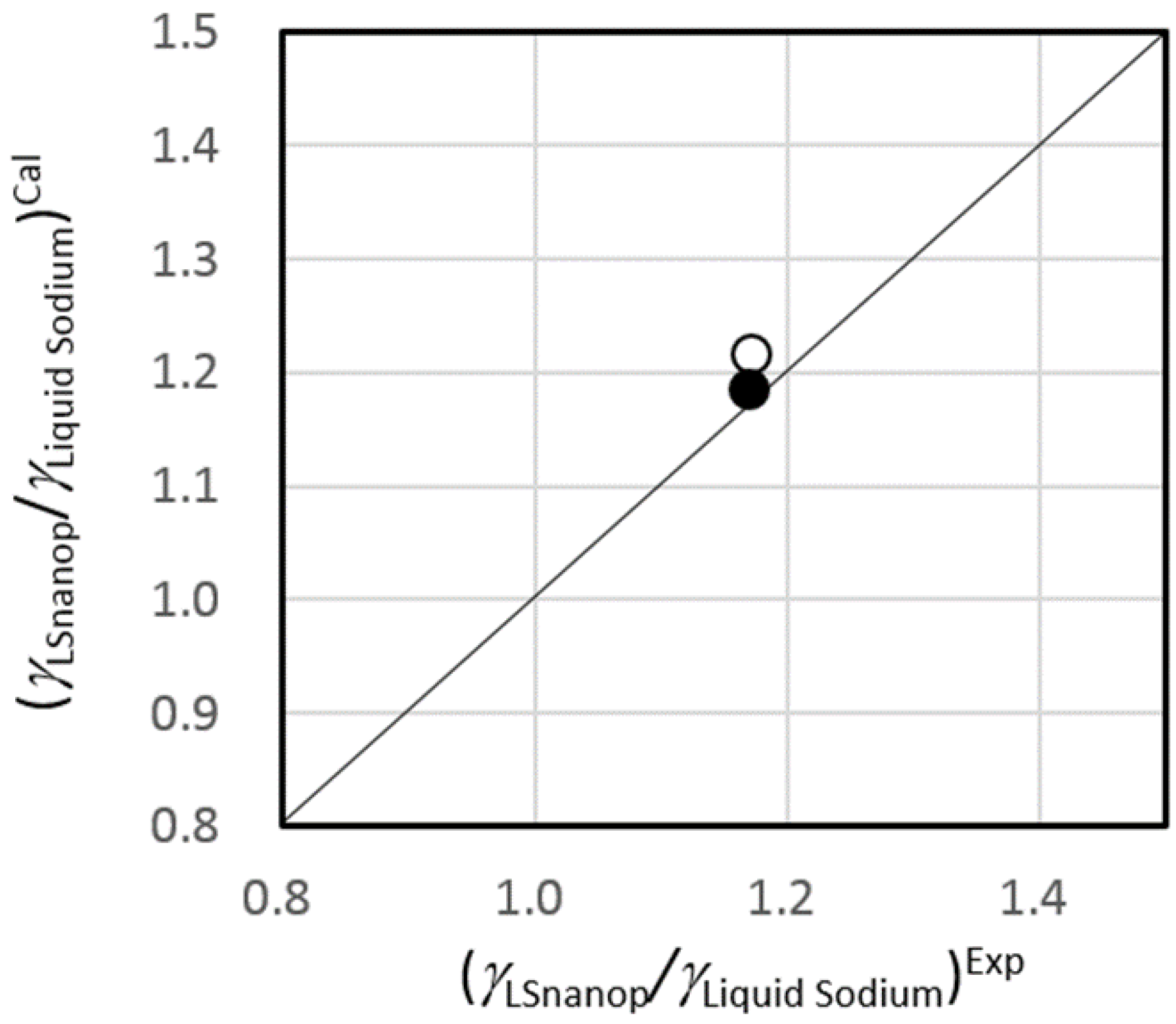
5.3. Surface Tension of LSnanop

Figure 6 shows the comparison of surface tension between the LSnanop and liquid Na in the temperature range from 500 to 873 K. The measured surface tension of liquid Na was in good agreement with the literature data [27]. This indicates the reliability of the measured data of surface tension and the adopted experimental method, the pendant drop image method [13]. The original data of surface tension was given as γ = −1.119 × 10⁻⁴ T + 0.2681 for the LSnanop and γ = −9.940 × 10⁻⁵ T + 0.2323 for liquid Na [13]. In these equations, the unit is N·m⁻¹ for the surface tension, γ, and K (Kelvin) for the absolute temperature, T. The surface tension of LSnanop is 17% larger than that of liquid Na, as can be seen in Figure 6 from the data points, which are situated far into the upper region in comparison to the slanted line. This increase of surface tension of LSnanop also implies the existence of excess cohesive energy, which is clarified experimentally in Section 5.4 and theoretically analyzed in Section 6.

Figure 6. Comparison of the surface tensions of LSnanop and liquid Na: The slanted line corresponds to the hypothetical case in which the surface tensions of LSnanop and liquid Na are equal.

Figure 6. Comparison of the surface tensions of LSnanop and liquid Na: The slanted line corresponds to the hypothetical case in which the surface tensions of LSnanop and liquid Na are equal.

The surface excess per unit area (or the surface adsorption) of Ti nanoparticles, Γ_Nano, can be estimated from the concentration dependence of surface tension. The Γ_Nano of LSnanop is related to the nanoparticle concentration (X_Nano) dependence of surface tension, γ. This relation is called the Gibbs adsorption formula [28], whose explicit form is written as follows:

$${\text{Γ}}_{Nano}=-\frac{1}{k_{B}T}\left(\frac{\partial \text{γ}}{\partial \ln X_{\text{Nano}}}\right)$$

(3)

The larger surface tension of LSnanop compared with liquid Na implies the negative adsorption for the surface layer of LSnanop; Ti nanoparticles are retired from the surface layer. The surface layer of LSnanop may only be covered with Na atoms. The completely inverse situation, positive adsorption, was concluded by a simple theoretical analysis ([1] p. 477) of the surface layer of liquid Hg-K alloys consistently with the concentration dependence of γ. The surface layer of K amalgam is covered with K atoms only, even if the atomic fraction of K is an order of 10⁻⁶ less. The negative adsorption, or the absence of Ti nanoparticles on the surface layer of LSnanop, may be deduced by a rather simplistic discussion of the surface layer of liquid mixtures. As is well known, the monolayer approximation is adopted for the Gibbs adsorption formula. Moreover, in the case of LSnanop, the size difference between constituents is extremely large, 5 nm radius for nanoparticles and 0.098 nm (ionic radius) and 0.154 nm (atomic radius) for Na [29]. Up to date, to the authors’ best knowledge, no surface structure analysis has been performed experimentally and theoretically for such mixtures whose size difference between constituents is as large as described above. This seems to be an interesting and important future subject in the surface science. At present, it may be considered that the Gibbs adsorption formula is grasping the essential point of LSnanop; namely, the surface layer of LSnanop may be covered only with Na atom.

It can easily be considered that the existence of excess cohesive energy may enlarge the surface tension of LSnanop. Empirically, the surface tension of liquid metals at the melting temperature is correlated with the heat of vaporization, ${\Delta }_l^g{H}_M$, and atomic volume, V_M, as follows [30]:

$$\text{γ}=1.8\times {10}^{-9}\frac{{\Delta }_l^g{H}_{\text{M}}}{{V_{\text{M}}}^{2/3}}$$

(4)

This relation was originally obtained for the surface tension γ_m of pure liquid metals at the melting temperature, γ_m. However, this relation is assumed to also be valid for liquid mixtures, such as the LSnanop. In the previous paper [13], Equation (4) has already been employed for the analysis of the effect of excess cohesive energy on the surface tension of LSnanop. Unfortunately, the excess cohesive energy was inserted into Equation (4) in place of the heat of vaporization. Therefore, once more, the analysis based on Equation (4) is performed with the use of the heat of vaporization. As described in Section 5.4, the excess cohesive energy of LSnanop is 19.8 kJ·molNa⁻¹, whose unit indicates that the system considered contains one mole of Na. Therefore, the heat of vaporization for the LSnanop is assumed to be 19.8 kJ·molNa⁻¹ larger than that of liquid Na (107 kJ·molNa⁻¹) ([30] p. 8). In Figure 7, a comparison of the ratio, γ_LSnanop/γ_{liquid Na} (γ_LSnanop: the surface tension of LSnanop; γ_{liquid Na}: the surface tension of liquid Na), is shown between the calculation by Equation (4) and the experimental value at the melting temperature. It may be possible to perform the comparison of this ratio of surface tension at any temperature. However, Equation (4) was originally presented for various liquid metals at their melting temperatures [30]. In addition, this ratio of surface tension is almost temperature independent, as can be seen from Figure 6. Therefore, this comparison was performed only at the melting temperature of Na. In Figure 7, the solid circle indicates the calculated result without atomic volume correction, in which only the correction of heat of vaporization is taken into account and the atomic volume of LSnanop is assumed to be same as that of pure liquid Na. The predicted ratio between the surface tension of LSnanop and that of liquid Na, 1.185, is in good agreement with the experimental ratio, 1.17, as can be seen from the solid circle close to the slanted line. It is very interesting that the agreement is worse in the case that the experimental value of atomic volume (shrinkage of 4.9%) is correctly inserted, as shown in Figure 7 by the open circle, which is apart from the slanted line. The calculated ratio of surface tension with atomic volume correction is 1.218. The better agreement with experiments for the prediction without atomic volume correction may correspond to the negative adsorption of LSnanop, which can be speculated from the 17% increase of surface tension with the addition of a small amount (X_Nano = 6.92 × 10⁻⁷) of Ti nanoparticles into liquid Na.

Figure 7. Comparison of the surface tension ratio (γ_LSnanop/γ_{liquid Na}) between the calculation by Equation (4) (indicated by “Cal”) and the experiment (indicated by “Exp”) at the melting temperature of Na; solid circle: the calculation without atomic volume correction; open circle: the calculation with atomic volume correction. The slanted line corresponds to the case on which the calculated values are same as experimental values.

Figure 7. Comparison of the surface tension ratio (γ_LSnanop/γ_{liquid Na}) between the calculation by Equation (4) (indicated by “Cal”) and the experiment (indicated by “Exp”) at the melting temperature of Na; solid circle: the calculation without atomic volume correction; open circle: the calculation with atomic volume correction. The slanted line corresponds to the case on which the calculated values are same as experimental values.

5.4. The Heat of Reaction to Water of LSnanop

In Figure 8 a comparison of the heat of reaction to water is shown between solidified LSnanop and solid Na. The heat of reaction to water of solidified LSnanop is smaller than that of solid Na, as can be seen from the data point, which is situated in the lower region below the slanted line. The data of heat of reaction to water were obtained for the solidified samples at 303 K, under a high purity argon gas atmosphere, using a Twin Conduction Calorimeter [13]. To perform this measurement, a LSnanop sample containing about 30 mg of Na (1.3 × 10⁻³ mole) was put in the sample capsule followed by the addition of 2 mL of water (0.11 mole). The calibration of the quantity of heat was performed by measuring the heat of reaction to water of sodium hydroxide (NaOH), whose literature data, −44.51 kJ·mol⁻¹ [31], is known. Because of the exothermic reaction of LSnanop to water, the temperature of the sample increased above the melting temperature of Na. Measured value of heat of reaction to water was corrected by taking into account of the heat losses due to the endothermic melting transition of Na. The employed value for the heat of melting of Na was 2.60 kJ·mol⁻¹ [32]. The measurements of the heat of reaction to water were repeated 32 times for the solidified LSnanop. The measurements were also repeated 19 times for solid Na. In addition, similar experimental results were obtained for the samples of liquid state at 373 K. Also in the liquid state, the decrease of heat of reaction to water of LSnanop was confirmed similarly to the experiments at the solidified state shown in Figure 8. After the measurements, the amount of Na and that of Ti were analyzed by using ICP-AES. In the previous paper [13], it was found that the obtained heat of reaction to water of solidified LSnanop, −156.9 ± 6.9 kJ·molNa⁻¹, is smaller as an absolute value than that of solid Na, −176.7 ± 4.9 kJ·molNa⁻¹. The experimental value for solid Na itself is in agreement with the literature value (−183.7 kJ·molNa⁻¹) [33], judging from the experimental error range. It is very important to compare the heat of reaction to water for a system containing the same amount of Na atoms between the solidified LSnanop and solid Na. Therefore, the heat of reaction to water is shown in units of kJ·molNa⁻¹ by calculating, from the measured heat value of the calorimetry and the number of Na atoms in the calorimetry sample, the quantity of heat corresponding to the system containing Na atoms of Avogadro’s number, N_A. The reproducibility of the experimental data was good. In addition, the thermal error sources, for example, the oxidation of impurities, were investigated in detail. Conclusively, there are no error sources to spoil the measurements of heat of reaction to water for the solidified LSnanop and solid Na. Therefore, a considerable reliability is present for the measured difference of heat of reaction to water, −19.8 kJ·molNa⁻¹, between the solidified LSnanop and solid Na. In the next section, this difference is thought to be derived from the existence of excess cohesive energy for the LSnanop.

Figure 8. Comparison of the absolute values of heat of the reaction to water between the LSnanop (solidified) and solid Na: The slanted line corresponds to the case in which the heat of reaction to water is the same for the LSnanop and liquid Na.

Figure 8. Comparison of the absolute values of heat of the reaction to water between the LSnanop (solidified) and solid Na: The slanted line corresponds to the case in which the heat of reaction to water is the same for the LSnanop and liquid Na.

6. Excess Cohesive Energy of LSnanop

6.1. The Determination of Excess Cohesive Energy of LSnanop from the Experimental Data of the Heat of Reaction to Water

It is very surprising that there exists a difference of the heat of reaction to water between solidified LSnanop and solid Na. Therefore, based on Hess’ law [34], the chemical reaction to water was investigated in detail. Conclusively, the existence of excess cohesive energy of LSnanop was found to be responsible for this difference [13]. The reaction to water of liquid Na is written as

Na + H₂O → NaOH + 1/2H₂:∆H^r(Na)

(5)

The chemical reaction to water of LSnanop is similarly written as follows:

Na(Ti) + H₂O → NaOH + 1/2H₂ + (Ti):∆H^r(Na(Ti))

(6)

In Equation (6), Na(Ti) and (Ti) indicate the LSnanop and Ti nanoparticles, respectively. The heats of reactions to water for both reactions, ∆H^r(Na) and ∆H^r(Na(Ti)), are, respectively, written as their enthalpies of constituent chemical components:

∆H^r(Na) = H_NaOH + 1/2H_H2 − H_Na − H_H2O

(7)

and

∆H^r(Na(Ti)) = H_NaOH + 1/2H_H2 + H_(Ti) − H_Na(Ti) − H_H2O

(8)

The heat of formation of LSnaop, ∆H^f(Na(Ti)), is defined by the following chemical equation.

Na + (Ti) → Na(Ti):∆H^f(Na(Ti))

(9)

Similar to Equations (7) and (8), the heat of formation of LSnaop, ∆H^f(Na(Ti)), can be written as follows:

∆H^f(Na(Ti)) = H_Na(Ti) − H_Na − H_(Ti)

(10)

Then, applying Hess’ law, the following equation can be obtained.

∆H^r(Na) − ∆H^r(Na(Ti)) = ∆H^f(Na(Ti))

(11)

Inserting the experimental values, −176.7 ± 4.9 kJ·molNa⁻¹ for ∆H^r(Na) and −156.9 ± 6.9 kJ·molNa⁻¹ for ∆H^r(Na(Ti)) into Equation (11), the heat of formation of LSnanop can be determined experimentally, as follows:

∆H^f(Na(Ti)) = −19.8 kJ molNa⁻¹

(12)

Thus, the enthalpy of solidified LSnanop is lower than the sum of enthalpy of solid Na and that of Ti nanoparticles. The similar lowering of enthalpy is also expected for the case of the LSnanop (liquid state) and liquid Na, as mentioned in Section 5.4. Therefore, we can consider the “excess cohesive energy” on the formation of LSnanop.

This result, Equation (12), seems to be valid, because in the analysis, based on the rigorous Hess’ law, there exists no suppositions except for the assumption that the condition of Ti nanoparticles is unchanged before and after the reaction. Though this assumption seems plausible, detailed discussions are given below. We note the experimental result that the heat of reaction to water for the solidified LSnanop is smaller as an absolute value than that of solid Na. This means that the difference between the enthalpy before the reaction to water and that after the reaction is smaller for the solidified LSnanop than for solid Na. This indicates two possibilities: the first possibility is the case in which the enthalpy after the reaction to water of the solidified LSnanop is larger (higher on the energy diagram) than that of solid Na, and the second possibility is the case in which the enthalpy before the reaction to water of solidified LSnanop is smaller (lower on the energy diagram) than that of solid Na.

We first consider the first possibility. A crystalline state can be considered for the Ti nanoparticles in the LSnanop with the evidence of the moiré fringe [13], as described in Section 8. If, after the reaction to water of solidified LSnanop, the crystalline state of Ti nanoparticles are changed into another state, such as an amorphous (non-crystalline) state (case A) or, in an extreme case, an independent atomic state (case B), the enthalpy after the reaction to water of solidified LSnanop may be increased. As a simplest approximation, the enthalpy of amorphous (non-crystalline) state may be assumed to be nearly the same as that of a liquid state. Therefore, the enthalpy increase of case A can be estimated by the heat of melting of Ti metal ([21] p. 11). This heat of melting, 4.45 kJ·mol⁻¹, and Ti concentration (2 at. %) gives the enthalpy increase of 0.396 kJ. This estimated value is far smaller than the 19.8 kJ·molNa⁻¹ given by Equation (12). Similarly, the enthalpy increase of case B can be estimated, as a simplest approximation, from the heat of vaporization of Ti metal ([21] p. 11). From the sum of the heat of melting, 4.45 kJ mol⁻¹, and the enthalpy of vaporization, 397 kJ·mol⁻¹, the increase of enthalpy after the water reaction can be estimated to be 8.02 kJ, which is far lower than 19.8 kJ·molNa⁻¹. We must remember that case B is a too extreme case. Even such an unlikely case can only explain 41% of the 19.8 kJ·molNa⁻¹ given by Equation (12). That is, it is very unlikely that the first possibility, the increase of the enthalpy after the reaction to water, is responsible to the origin of the difference of the enthalpy of reaction to water between the solidified LSnanop and solid Na. Thus, it may be allowed to assume that the condition of Ti nanoparticles may be unchanged. Of course, further detailed experimental studies must be done for the characterization of Ti after the reaction to water of solidified LSnanop, though the preliminary studies were performed for the reaction products, as described in Section 5.

Thus, only the second possibility may be important: The difference of heat of reaction to water may be derived from the difference of the initial state (before the reaction to water) between the solidified LSnanop and solid Na. The enthalpy of solidified LSnanop seems to be smaller than the simple sum of the enthalpy of solid Na and that of Ti nanoparticles. Thus, the formation of LSnanop from liquid Na and Ti nanoparticles is an exothermic reaction. At present, the authors believe that the negative heat of formation may be derived from the existence of the excess cohesive energy for the LSnanop, defined by Equations (9) and (10). The existence of excess cohesive energy may be also supported by the shrinkage of atomic volume (Section 5.1) and the increase of surface tension (Section 5.3). This excess cohesive energy corresponds to 3.3% of the cohesive energy of liquid Na ([2] p. 110). Therefore, in the next section, the origin of this excess cohesive energy is discussed from the theoretical point of view.

6.2. Theoretical Analysis of Excess Cohesive Energy of LSnanop

It seems to be clear, from the experimental point of view, that the excess cohesive energy for the LSnanop exists. To the best of the authors knowledge, this experimental discovery of excess cohesive energy is the first case in the field of colloidal solutions or suspension liquids, though inter-particle interactions have been discussed traditionally by the so-called DLVO (Derjaguin, Landau, Vervey, and Overbeek) theory [35]. The DLVO theory considers the problem of aggregation of charged colloidal particles by the inter-particle potentials derived from the Coulomb repulsion (short distance) and the van der Waals’ attraction (long distance). However, in the case of LSnanop, the role of conduction electron must be considered in any method. Thompson [36] performed the first theoretical discussion of the interaction of suspended metallic bodies in a liquid metal medium. His analysis was essentially based on the DLVO theory. In Thompson’s analysis, the inter-body interaction was taken into account by the theory of Hamaker [37] and Lifshitz [38] based on the van der Waals’ interactions. In addition, the existence of conducting medium was considered by taking into account the screening effect caused by the electron gas. Kim et al. [15] presented a similar approach for the inter-particle interaction of LSnanop. The effect of the existence of conduction electrons is taken into account by the ab initio DFT (density functional theory) calculation, which is also discussed in detail in Section 8.

The essential feature of LSnanop may exist in the problem of bimetallic interface, which has been discussed based on the density functional theory [39] and the periodic planar jellium approximation [40]. In the case of a Na-Al bimetallic interface, with a large difference of electronegativity, the electron transfer was predicted to occur from Na (0.93) with a smaller electronegativity to Al (1.61) with a larger one [39]. The numerical value in the parentheses indicates the Pauling’s electronegativity [41]. Therefore, the electron transfers may occur from liquid Na (0.93) to Ti nanoparticles (1.54). These electron transfers produce the electrical double layer in the interfacial region. Such an effect contributes to the interfacial energy as the electrostatic energy. Lang and Kohn [42] performed a jellium model analysis of surface energy based on the inhomogeneous electron gas theory. They showed that the contribution of this electrostatic energy is 25% of the surface energy in the case of electron density corresponding to Na metal. Based on the knowledge described above, the excess cohesive energy of LSnanop is discussed below.

6.2.1. The Analysis Based on the Born Model

Because of the charge transfer from liquid Na to Ti nanoparticles, Ti nanoparticles carry negative charges derived from the transferred electrons. These negatively charged nanoparticles are screened by the removal of conduction electrons or the positively charged Na⁺ ions. This situation can be approximately considered by the Born model [43], which successfully reproduces the solvation energy of charged ions in electrolyte solutions or water. In this review, some attempt has been made to apply the Born model to the LSnanop.

The assembly considered contains N_Nano ions immersed in a medium whose dielectric constant is ε_r, which is defined by the ratio of dielectric constant of material, ε, to that of vacuum, ε₀. Each ion (nanoparticle) has an electric charge, $-\Delta Z\left|e\right|$ and radius, r_N; the symbol $\left|e\right|$ is the absolute value of electronic charge. According to the Born model [43], which was derived from the charging process for ions of interest, the stabilization of these ions in the dielectric medium is evaluated by the following gain of Gibbs free energy due to the solvation.

$${\Delta }_{sol}G=-\frac{\Delta Z^2{\left|e\right|}^2{N}_{\text{Nano}}}{8{\text{πε}}_0(r_N)}(1-\frac{1}{{\text{ε}}_r})$$

(13)

In principle, the solvation of positive Na⁺ ions should also be considered. However, it can be shown that the solvation energy of positive Na⁺ ions can be neglected. As for the ε_r, ε_r = 8 was assumed for a rough estimation, consulting the data of Ag [44], though some arbitrariness is included due to its wave length dependence. Thereefore, we use the Equation (13) as the starting point of the consideration for the screening effect in the LSnanop. If the value of ∆Z is known, the stabilized energy due to the solvation can be estimated. At present, no rigorous method is present for the estimation of ∆Z. Therefore, the previous knowledge and the studies are employed for the estimation of the number of transferred electrons per Ti atom, ∆n [13]. The ∆n is related to ∆Z with the relation, ∆Z = n_Ti∆n; the symbol n_Ti means the number of Ti atoms in one Ti nanoparticle, as defined in Section 4. The value of ∆n is given to be 0.10 (case A) from the Pauling’s diagram [41], by which the degree of ionic character can be estimated by the knowledge of the electronegativity difference between constituent elements. This method was originally proposed for a diatomic molecule. The value of 0.05 (case B) was also estimated for ∆n from the ab initio calculation of VASP (Vienna Ab initio Simulation Package) code for the model of an Na-Ti-Na sandwich system [9], and the value of 0.22 (case C) was also given from the calculation due to the DFT for the Na atom–Ti cluster system [12]. These three cases give, respectively, −74.2 kJ·molNa⁻¹ (case A), −18.6 kJ·molNa⁻¹ (case B) and −359.1 kJ·molNa⁻¹ (case C) as the gain of Gibbs free energy, according to Equation (13). The calculation of case B is in the best agreement with the experimental value, −19.8 kJ·molNa⁻¹. The value of ∆Z, which reproduces the experimental value of excess cohesive energy, −19.8 kJ·molNa⁻¹ by Equation (12), is 1.54 × 10³. The corresponding value of ∆n is 0.052. The Born model tells us that the solvation or screening effect is important for the excess cohesive energy of LSnanop.

6.2.2. The Screened Nanoparticles with Negative Charge in Liquid Sodium (SNP in Liquid Na)

The screening effect must be considered for the negatively charged nanoparticles of Ti under the influence of a plentiful amount of conduction electrons derived from the liquid Na medium. Unfortunately, no theory is available to apply to the LSnanop. The van der Waals interaction, which is one important basis of the standard theory of colloidal or suspension liquids, DLVO theory, does not always seem valid for the excess cohesive energy of a metallic system, such as LSnanop. Under these conditions, the excess cohesive energy of LSnanop was considered based on the proposed model, the screened nanoparticles with negative charge in liquid sodium (“SNP in liquid Na”) [13], though it remains a crude approximation. First, the Ti metal has been considered to be a monovalent metal [45], similar to liquid Na. Therefore, only transferred electrons to Ti nanoparticles from liquid Na can be treated as an excess charge if they are observed from their outside region. Then, we consider the screening of negatively charged Ti nanoparticles in liquid Na. The excess charge in metals is always screened quickly by a plentiful amount of conduction electrons. Around the positively charged particle or positive ion, the conduction electrons gather in the surrounding narrow range to cancel their excess charge. For example, the screening distance is 0.068 nm for metallic sodium [46]. However, the screening of a negatively charged particle is different from that of a positively charged one. The screening of a negatively charged particle in liquid Na medium is only possible by exposure to positive Na⁺ ions in its surrounding region. This can be established by the retirement of conduction electrons from this surrounding region. The screening distance for the negative charge may be larger than that for the positive one because of the reason that the size of electron is thought to be absent and that of positive Na⁺ ion is finite. Therefore, it can be assumed that the negatively charged nanoparticle of Ti always accompanies the screening shell of finite thickness, r_OSC −r_N, in which r_OSC is the outer boundary radius of screening shell and r_N is the radius of the nanoparticle.

In this screening shell, there are no conduction electrons and, as a result, positive ions are assumed to be exposed to a uniform density of ρ₊ (jellium model for positive ions). Then, the attractive energy, ∆E_SC, appears between the negatively charged Ti nanoparticle and the positively charged screening shell. The repulsive energy, ∆E_REP, also works among transferred electrons on the Ti nanoparticle from liquid Na. The inter-nanoparticle interaction can be assumed to be neglected due to the complete screening. In the SNP in liquid Na model, the consideration is not necessary for the repulsive interaction among positive ions in the screening shell, because its appearance is cancelled by the disappearance of repulsive interactions among conduction electrons in this region. Under the assumptions described above, the excess cohesive energy, ∆E, can be written as the sum of ∆E_SC and ∆E_REP.

∆E = ∆E_SC + ∆E_REP

(14)

The transferred electrons on Ti nanoparticles may be rather localized in the d-band or may be itinerant in the sp-d overlapping band [45] of nanoparticles. For simplicity, in the present model, transferred electrons are assumed to be distributed uniformly (free electron) on the Ti nanoparticles. Then, the LSnanop contains N_Nano nanoparticles of Ti in liquid Na. By the charge transfer, each Ti nanoparticle of radius r_N possesses an excess charge, $-\Delta Z\left|e\right|$, in which $\left|e\right|$ is the absolute value of the electronic charge. The movement of conduction electrons in liquid Na screens this transferred excess charge in Ti nanoparticles quickly. The excess negative charge, $-\Delta Z\left|e\right|$, itself should be determined by the condition that the chemical potential, or the Fermi energy, of Ti nanoparticle must be equal to that of liquid Na medium. In the present study, it is assumed that the employed magnitude of $-\Delta Z\left|e\right|$ has already been determined in this manner. Under the given $-\Delta Z\left|e\right|$, the energy change on the formation of LSnanop, or the excess cohesive energy, can be considered based on the free electron model for excess electrons on Ti nanoparticles and the jellium model of the number density, ρ₊, for Na⁺ ions in the screening shell.

By following Raims’ procedure ([2] p.109), the repulsive energy among negative charges on the Ti nanoparticles, ∆E_REP, can be given for the LSnanop. The explicit form is given as follows:

$$\Delta E_{REP}=N_{\text{Nano}}\frac{1.2{\left(\Delta Z\right)}^2}{r_N}$$

(15)

By using Gauss’ theorem, the expression for the attractive energy between the negatively charged nanoparticle and the positively charged screening shell, ∆E_SC, is given as

$$\Delta E_{SC}=-N_{\text{Nano}}4\text{π}(\Delta Z){\text{ρ}}_{+}(r_{OSC}^2-r_N^2)$$

(16)

The condition for the complete screening of every Ti nanoparticle by its screening shell is written as follows:

$$\Delta Z=\frac{4}{3}\text{π}(r_{OSC}^3-r_N^3){\rho }_{+}$$

(17)

It can be assumed that the thickness of the screening shell is thin. Therefore the attractive energy, ∆E_SC, is written as

$$\Delta E_{SC}=-N_{\text{Nano}}\frac{2{\left(\Delta Z\right)}^2}{r_N}$$

(18)

Hence, the excess cohesive energy of LSnanop, ∆E, can be written as follows:

$$\Delta E=-N_{\text{Nano}}\frac{0.8{\left(\Delta Z\right)}^2}{r_N}$$

(19)

The Rydberg energy unit was employed in Equations (15)–(19).

If the number of transferred electrons on the Ti nanoparticle from liquid Na, ∆Z, is known, the excess cohesive energy of LSnanop can be calculated by the “SNP in liquid Na” model. The previous three cases for ∆n or ∆Z are once again adopted (∆Z = n_Ti∆n). The ∆n = 0.10 (case A), which is estimated from the Pauling’s diagram [41], gives −84.9 kJ molNa⁻¹. The ∆n = 0.10 (case B), which is derived from the ab initio MD (molecular dynamics) simulation for the model of Na-Ti-Na sandwich system [9], provides −21.2 kJ·molNa⁻¹. The ∆n = 0.22 (case C), which is derived from the DFT calculation for the Na atom–Ti cluster system [12], gives −410 kJ·molNa⁻¹. The calculated result of case B is in the best agreement with the experimental excess cohesive energy. The value ∆n = 0.048 is obtained to reproduce the experimental excess cohesive energy, −19.8 kJ·molNa⁻¹ according to Equation (19). Thus, a similarly good result was obtained between the Born model and the “SNP in liquid Na” model. This implies the importance of the screening of negatively charged nanoparticles by the positive charges.

The “SNP in liquid Na” model seems to be based on too many simplistic assumptions, such as uniform distribution of transferred electrons on the Ti nanoparticle, the jellium model for Na⁺ ions in the screening shell, the equality of the excess negative charge on Ti nanoparticles to the transferred electrons from liquid Na, etc. However, the distribution of transferred electrons on the Ti nanoparticles can be assumed to be uniform with consideration of the Coulomb interactions, even if they are in d-states (or d band) of Ti. This assumption may be supported, at least for the evaluation of ∆E_SC, because of Gauss’ theorem. In addition, at least the jellium model was successfully adopted for the explanation of the magic number of nanoparticles [47] and the surface energy of metals [42]. The assumption about excess negative charges on the Ti nanoparticle may also be supported by the study of electron transport properties of liquid transition metals, which states that the valence of liquid transition metals can be considered to be monovalent in the nearly free electron model [48], similar to the case of solid transition metals [45], though some arbitrariness has been reported for the valence of liquid transition metals [49]. These points are to be discussed elsewhere in near future.

In the “SNP in liquid Na” model [13], the inner boundary and the outer one of the screening shell are assumed to be sharply defined. However, an oscillatory behavior has been found for the electron density profile in the metallic interface in many previous theoretical calculations [39,40,42] based on precise quantum mechanical theories. It may be possible to assume a decaying function of oscillatory behavior for the electron density profile of excess charge on the theoretical analysis. Though this oscillatory behavior may be derived essentially from the wave nature of electrons, in the present “SNP in liquid Na” model, the sharply defined boundary of screening shell was simply adopted as a simplest approximation for a rather long screening distance of the negatively charged nanoparticles. Therefore, the contribution of electron density profile at the boundary was neglected for the estimation of excess cohesive energy. This simplification may be possible because of the reason that the Coulomb energies, ∆E_SC and ∆E_REP, may be dominant compared to the contribution of electronic structure for the considerably large charge transfer case. Such a simplification was also adopted for the theoretical analysis of the isolated Coulomb fission of charged nanoparticles ([47] p. 78), referred to in Section 8.

Furthermore, the contribution of difference of work function, or contact potential, was not considered explicitly in the “SNP in liquid Na” model [13]. This contribution was not so dominant for the surface energy of metallic Na [42]. As for the electrostatic contribution of interfacial effect or double layer, it is possible to consider that it may be partially taken into account in the “SNP in liquid Na” model. Until now, in this model many challenging subjects to be resolved remain, such as the incorporation in a self-consistent manner of the profile of electron density in the Ti nanoparticles and around their boundary regions, the distribution of Na⁺ ions around the screening layers, and the difference of work functions between constituent species. These subjects may be resolved by the application of an ab initio DFT calculation of electronic structure for the LSnanop. As already described, the system size of LSnanop is still considerably large for an ab initio DFT calculation. We believe that some essential points are included in the “SNP in liquid Na” model. Therefore, it is very important to solve the charge transfer per atom (nanoparticles) and the excess cohesive energy in a self-consistent manner in the “SNP in liquid Na” model. Anyway, it is important, for the better understanding of LSnanop, to improve this model by incorporating the subjects described above, together with the endeavor for an ab initio DFT calculation and MD simulation. The “SNP in liquid Na” model reminds us of the idea of Popplewell et al. [50]: the space charge layer coating, or the Coulomb repulsive layer coating. The fitted value to Equation (19), ∆n = 0.048, corresponds to a depth of 0.195 nm for the positively charged Na⁺ screening shell. In Ref. [13], the thickness of the screening shell was given as 0.20 nm due to the slightly different input data. The contribution of screening shell to the stability of LSnanop is discussed later (Section 8).

To end this section, a summary is given below for the process along which the excess cohesive energy may be considered to exist in the LSnanop.

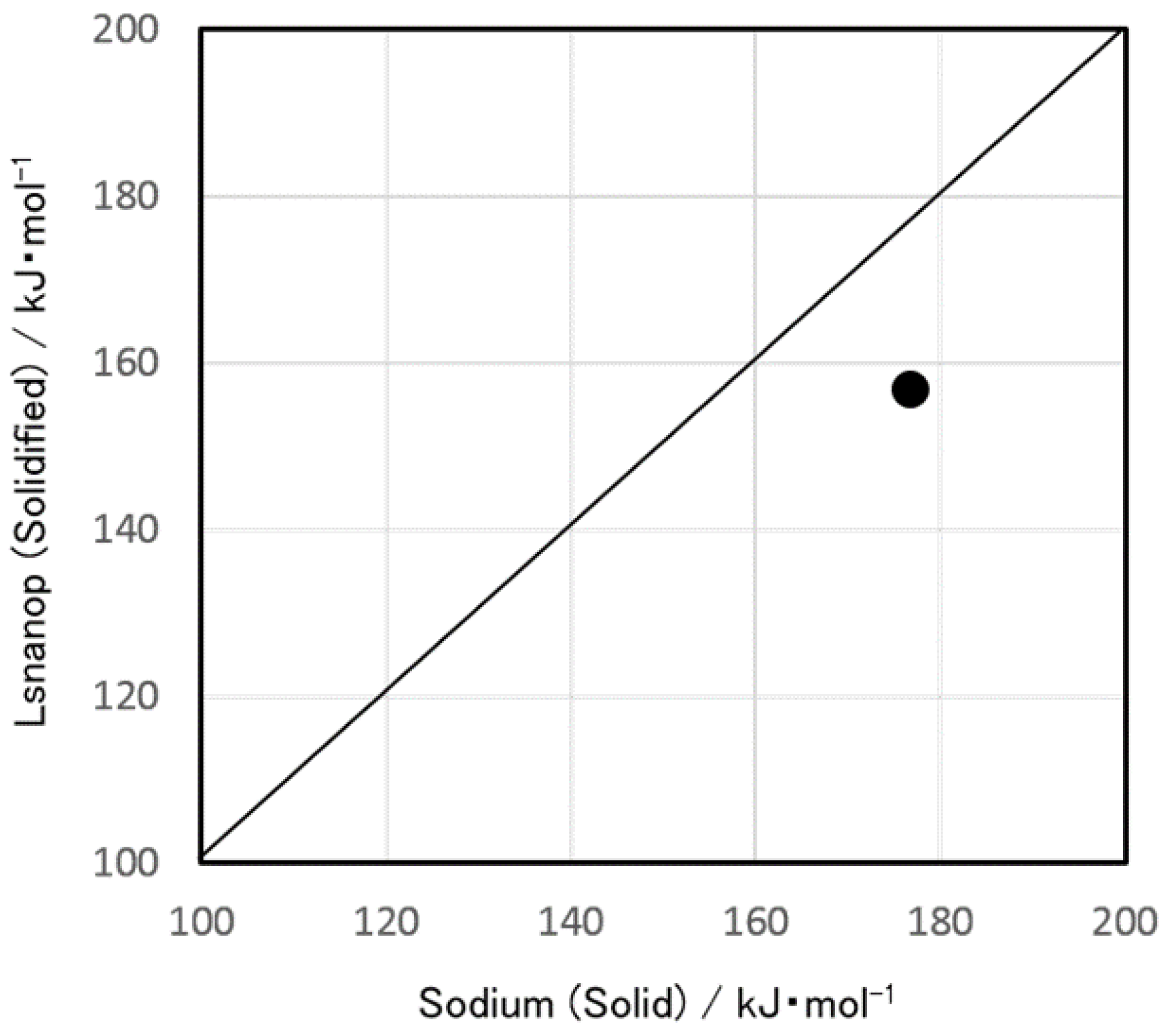
• Experimentally, a difference of heat of reaction to water was found between solidified LSnanop and solid Na. This experimental result is reliable, judging from the reproducibility of experiments and the preliminary error analysis of the thermal analysis.
• A similar decrease in the heat of reaction to water of LSnanop was also confirmed experimentally for the samples in a liquid state.
• The decrease of heat of reaction to water of LSnanop seems to be derived, not from the raise of the enthalpy of final state, but from the lowering of the enthalpy of initial state before this reaction.
• Based on Hess’ law, this difference is thought to be derived from the existence of excess cohesive energy for the LSnanop. Hess’ law is a rigorous law in thermodynamics based only on the fact that the enthalpy is a quantity of state.
• The experimentally estimated excess cohesive energy can be explained theoretically by the Born model and the “SNP in liquid Na” model. The transfer of electrons to Ti nanoparticles from Na atoms, which is the fundamental viewpoint of these models, is revealed by the ab initio DFT calculation [12] and ab initio MD simulation [9].

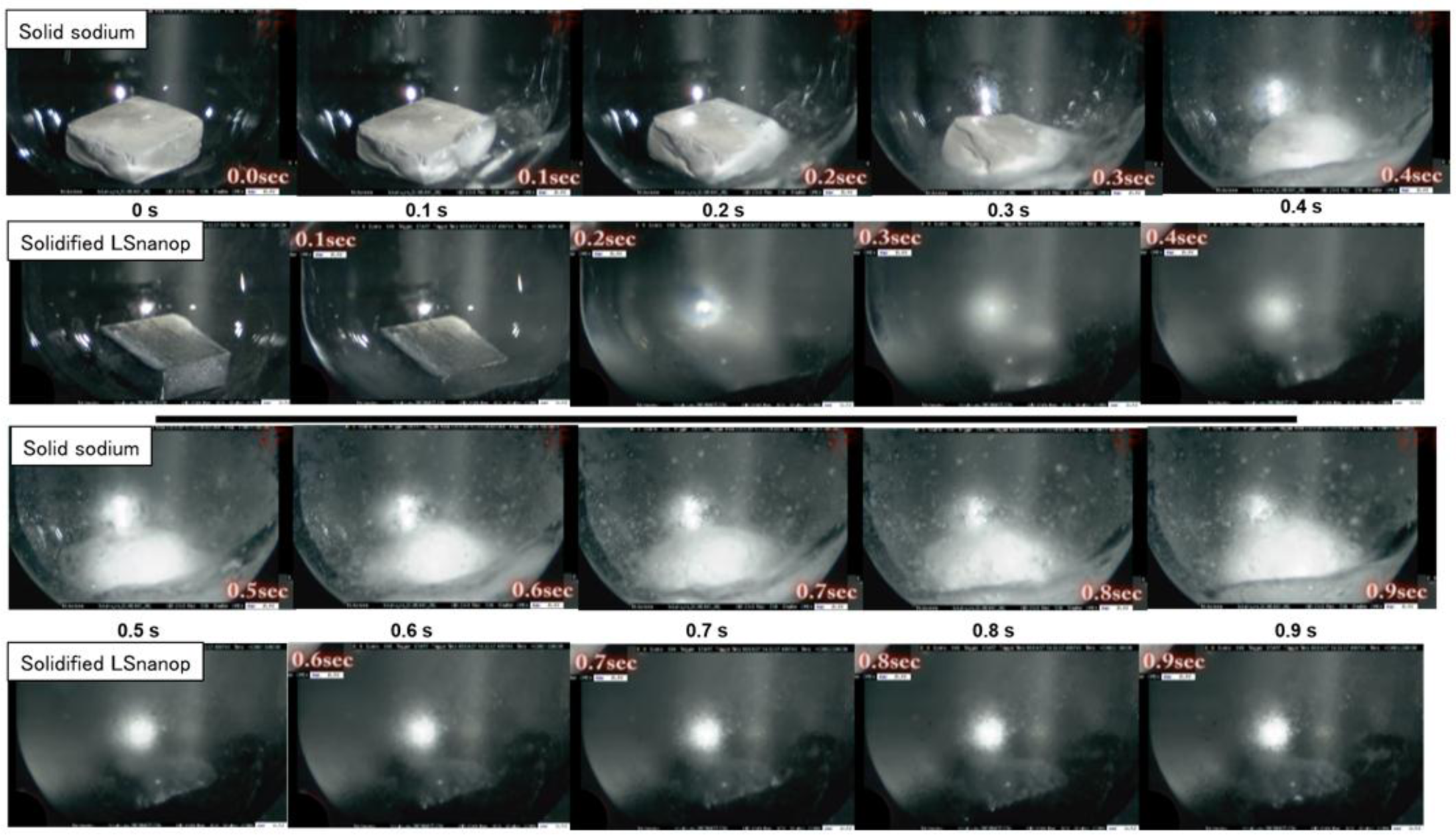
7. The Suppression of Reaction to Water and Oxygen of LSnanop

As already described, the generated heat on the exothermic reaction to water of solidified LSnanop is smaller than that of solid Na. This leads us to expect the possibility of suppression of chemical reactivity to water and oxygen. This suppression of chemical reactivity was investigated in Refs. [11,14]. In this Section is given a review of this subject, in which new important factors to be considered are pointed out.

7.1. The Suppression of Reaction to Water

Figure 9 shows a photographic comparison between the time variation of reaction to water for the solidified LSnanop and that for solid Na in the interval from the onset of reaction to 0.9 s after the onset. The hydrogen bubbles generated by the reaction (Equation (5) or (6)), are observed as the white part in water on the surface of the sample in these photographs. In the case of solid Na, the reaction to water becomes remarkable at 0.3~0.4 s and continues until 0.9 s, the end of experimental time, with an almost constant vigor. On the other hand, in the case of solidified LSnanop, the reaction to water is far milder compared to the solid Na case over the whole experimental interval. This difference of reactivity to water should be studied in detail. The accumulation of Ti nanoparticles on the surface layer of LSnanop may play an important role in the suppression of chemical reactivity to water. Ara et al. [11] investigated the time variation of hydrogen pressure generated by the reactions (Equations (5) and (6)). The water is dropped from a nozzle to the solid Na in a vessel. A similar experiment was also performed for solidified LSnanop. In the case of solid Na, in the first stage, the hydrogen pressure increased abruptly up to the maximum value with an almost constant increasing rate; then, it remained at an almost constant value until the end of the experimental time. On the other hand, in the case of solidified LSnanop, in the initial short period (first stage), the hydrogen pressure increased abruptly, similar to the solid Na case; however, in the second stage, the hydrogen pressure was suppressed, though its increasing tendency continued; and in the third stage this increasing tendency became moderate and it took a long time for the hydrogen pressure to reach the maximum pressure, which was the same as the maximum pressure for the solid Na case. These behaviors also clearly show the suppression effect of LSnanop to the chemical reaction to water. It is important to clarify the role of Ti nanoparticles in the reaction interface of chemical reaction to water. It should be noted that the experiments for the reaction to water were performed in the solid state due to the reaction rate being too fast. In the case of the liquid state experiments, the difference of surface tension and the negative adsorption in the LSnanop may play a significant role in the difference of reactivity to water between LSnanop and liquid sodium. A detailed discussion is to be given elsewhere for the difference of mechanism of the reaction to water between LSnanop and Na. The suppression of reaction to water for the LSnanop is a significant advantage for the safety of heat exchange system composed of liquid Na and water, for example, for fast reactor technology.

Figure 9. A comparison of the reaction to water between the solidified LSnanop and solid Na.

Figure 9. A comparison of the reaction to water between the solidified LSnanop and solid Na.

7.2. The Suppression of Reaction of LSnanop to Oxygen

Figure 10 shows the photographic comparison of the time variation of burning, or reaction to oxygen, between the LSnanop and liquid Na in the time interval from the onset of burning to 20 s after the onset. The burning experiment was performed by using a gas mixture of N₂-20 vol. % O₂. The initial temperature of the sample pool was kept at 773 K. In the case of liquid Na, the burning continues up to the final experimental time, 20 s. Observing Figure 10 in detail, the burning of liquid Na seems to be the hardest at 4 s, followed by a slightly moderate decrease of vigor until 20 s. On the contrary, the burning of LSnanop becomes weaker at 4 s, and almost stopped at 10 s. That is, the capability of self-extinction for the LSnanop was found to exist.

Figure 10. A comparison of reaction to oxygen between the LSnanop and liquid Na.

Figure 10. A comparison of reaction to oxygen between the LSnanop and liquid Na.

The integrated heat of combustion was also measured with the use of a specially designed apparatus [11]. The Na sample weight was 2 g. Figure 11 shows a comparison of the integrated heat of combustion [11] between LSnanop and liquid Na. Until 1.5 min from the onset of burning, the heat generation was the same for LSnanop and liquid Na. However, at 2 min, the integrated heat of combustion for the LSnanop was decreased to be 75% of that for liquid Na. At 3 min, this decrease of generated heat was 68%.

Figure 11. A comparison of the integrated heat of combustion between the LSnanop and liquid Na: The slanted line indicates the hypothetical case in which the integrated heat of combustion is same for the LSnanop and liquid Na.

Figure 11. A comparison of the integrated heat of combustion between the LSnanop and liquid Na: The slanted line indicates the hypothetical case in which the integrated heat of combustion is same for the LSnanop and liquid Na.

Nishimura et al. [14] provided a detailed explanation of the difference of burning tendency between LSnanop and liquid Na. There are too many factors that relate to the burning phenomena, as described in Ref. [14]. Here, only important points and new views are explained. The burning mechanism is schematically shown in Figure 12. In the case of liquid Na, the connection of a channel in the oxide layer (or column) grows at the crack of the oxide film. Liquid Na is pumped up through these channels to the top of the oxide layer, at which the burning occurs. Together with the progress of burning, the temperature of liquid Na is increased. This causes an increase on the solubility of oxygen in liquid Na and a decrease of surface tension, which causes an increase on the spread of liquid Na at the outlets of channels on the top of the oxide layer. At these outlets, burning occurs in terms of the evaporation of liquid Na, which proceeds significantly at higher temperatures. Thus, the burning phenomenon grows violently with the progress of burning. On the other hand, in the case of LSnanop, as shown in Figure 12, some channels are blocked by Ti oxide plugs (blue bars in Figure 12). These Ti oxide plugs are formed in the channel by the oxidation of Ti nanoparticles; oxygen is supplied from the dissolved oxygen in liquid Na or the gas transport of O₂ from the atmosphere through the fine pores or fine cracks of the oxide layer (or column). Thus, the transport of liquid Na through the channel is interrupted by these plugs. As a result, the burning at the top part of the oxide layer is suppressed.

Therefore, in the case of LSnanop, the temperature is kept low and the solubility of oxygen in liquid Na is also kept low. This keeps the surface tension of liquid Na large. As a result, the spread of liquid Na is limited at the outlet of channel on the top of the oxide layer. Thus, the burning is limited due to the decrease of the evaporation of liquid Na. In the extreme case, self-extinction occurs. The negative adsorption of LSnanop seems to work effectively for the formation of Ti oxide plugs because, in the inside of LSnanop, Ti nanoparticles are enriched due to the retirement of Ti nanoparticles into the inside of LSnanop.

Figure 12. A comparative schematic of the reaction to oxygen of LSnanop and liquid sodium; blue bars: titanium oxide plugs; small dots of red and bitter orange: burning points.

Figure 12. A comparative schematic of the reaction to oxygen of LSnanop and liquid sodium; blue bars: titanium oxide plugs; small dots of red and bitter orange: burning points.

Here, authors stress that many Ti oxide plugs are not always required for the suppression of burning. The liquid Na is supplied through the inter-dendritic channel up to its outlet on the top of the oxide layer, at which burning occurs. The inter-dendritic channel is composed of many branches and turning points, as shown in Figure 12. According to the percolation theory, obstruction of the supply of liquid Na up to the burning site at the top is realized if only some branches, for example, 17% [51,52,53,54], are blocked by Ti oxide plugs. This is the reason why a small amount of Ti nanoparticles in the LSnanop is very effective in the suppression of burning. In other words, the role of Ti nanoparticles may be very effective for the self-extinction of burning.

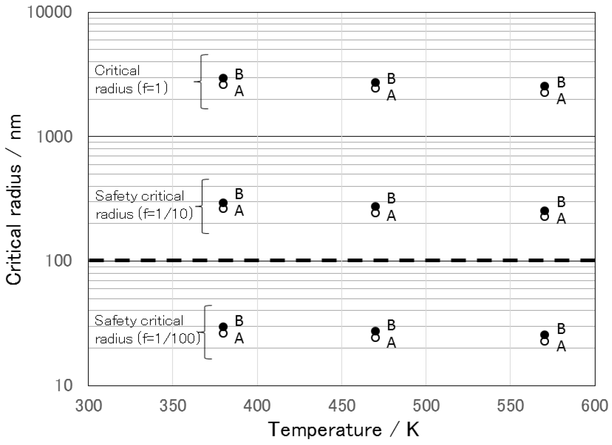
8. The Stability of LSnanop

The LSnanop contains some difficult points as a suspension liquid: the density difference between liquid Na and Ti nanoparticles is large; and it is almost impossible to adopt surface coating, which has been applied to magnetic fluids and in which suspended particles are coated with organic molecules with long bond chain to reduce the aggregation and the sedimentation and to improve the lyophilic property. Nevertheless, the LSnanop seems to be a very stable suspension liquid. Therefore, the stability of LSnanop must be discussed in detail. One important reason for this stability seems to be the existence of excess cohesive energy. The stability of LSnanop seems to be guaranteed thermodynamically by lowering (or the stabilization) of its energy state. The suspension mechanism due to the Brownian motion works effectively for particles of nanometer size, such as Ti nanoparticles in liquid Na in the case of LSnanop. Due to the absence of mutual solubility between liquid Na and Ti nanoparticles, the mechanism of Ostwald ripening does not work; Ostwald ripening is caused by the curvature dependence of chemical potential of matter. By this mechanism, small particles dissolve into a liquid medium and large particles grow. The LSnanop is irrelevant to this mechanism. The very dilute concentration of Ti nanoparticles in the LSnanop also has the advantage of the inhibition of mutual collision and the agglomeration of Ti nanoparticles, and the sedimentation due to such aggregations.

In addition, the existence of excess cohesive energy leads to the LSnanop being more stable by another mechanism, the space charge layer coating, or the Coulomb repulsive layer coating, which was proposed by Popplewell et al. [50]. They planned the improvement of suspension tendency by the Na addition to an Hg based ferrofluid containing Fe particles. The formation of a Na⁺ layer around Fe particles was expected to keep the inter-particle distance larger due to the Coulomb repulsion among Na⁺ layers. The “SNP in liquid Na” model tells us the possibility that each Ti nanoparticles of 10 nm is coated with the positively charged screening shell of 0.195 nm thickness, as described in Section 6.2.2. It is possible to consider that the Coulomb repulsive layer coating seems to be realized in the LSnanop.

The excess cohesive energy of LSnanop is derived from the charge transfer from liquid Na to Ti nanoparticles. As is well known, the accumulation of electric charge with the same sign causes the Coulomb fission. On the other hand, from Equation (19), any charge transfer gives the negative value of excess cohesive energy. Therefore, the Coulomb fission may be irrelevant to the LSnanop. However, because the theory of excess cohesive energy of LSnanop, Equation (19), is still in a very primitive stage, the possibility of Coulomb fission must be discussed a little in detail from another point of view [13]. The Coulomb fission has been reported for liquid drops of isolated metallic nanoparticles experimentally and theoretically [47(p. 78),55,56]. For example, the fission event in vacuum, Ag₂₁²⁺ →Ag₉⁺ +Ag₁₂⁺, was reported [57,58]. In this equation, the Coulomb fission occurs around the critical ratio, z/N = 0.095 (z: charge on nanoparticles in unit of the electronic charge, $\left|e\right|$; N: number of atoms). In addition to the existence of excess cohesive energy, also from the ratio, z/N ≈ 0.05, given by fitting Equation (19) to the experimental excess cohesive energy, may indicate the absence of Coulomb fission, judging from this critical ratio. The Coulomb fission event was originally obtained for isolated “charged liquid drop” of metallic nanoparticles. It is well known that, with the decrease of diameter of nanoparticles, particularly under 10 nm, the melting temperature, T_m, decreases abruptly and is far lower than the T_m of bulk metals [59,60]. Therefore, there is the possibility that the Ti nanoparticles in the LSnanop may be melted, or at least surface softening may occur. In the TEM image of solidified LSnanop, the moiré fringe was found on the Ti nanoparticles [13]. This fact may indicate that the Ti nanoparticles in the LSnanop may be present in a crystalline state. This discussion also weakens the possibility of Coulomb fission. The LSnanop seems to be free from such a Coulomb fission. In addition, the existence of excess cohesion energy, given by Equation (19), also serves to keep the essential stability of LSnanop without the Coulomb fission.

Recently, Kim et al. [15] studied theoretically the stability of LSnanop in terms of the inter-nanoparticle interaction between Ti nanoparticles with 10 nm diameter in liquid Na. They assumed that the major interactions are the van der Waals interaction of Hamaker type [37] and the solvation potential. The solvation potential between spherical Ti nanoparticles was evaluated by the Derjanguin approximation [61]. The force exerted on Na atoms from the surface of Ti nanoparticle was needed for this approximation. This was calculated by the ab initio DFT (density functional theory). The model system was composed of one Na atom and 60 Ti atoms in five layers, in which the first three layers near to Na atom were relaxed and the next two layers were taken to be the same as bulk Ti. The total interaction between Ti nanoparticles shows that an attractive interaction works only when the distance between Ti nanoparticles is very short and the repulsive interaction works in almost all ranges of inter-particle distance. The maximum height (barrier) becomes about 9630 k_BT, which means that no aggregation occurs. This result seems to guarantee the stability of LSnanop. The large repulsive inter-particle interaction may be caused by the overlapping of solvation layers. It is very interesting, from such an ab initio theoretical study, to reveal the vivid pictures for the origin of this large barrier against the mutual approach of Ti nanoparticles, the solvation, the degree, and the role of charge transfer, the role of screening effect due to the conduction electrons.

At present, some experimental evidence has been obtained for the long-term stability, which is extremely important in a thermal medium for the practical operation of technologies requiring highly efficient heat removal, such as fast reactors. One piece of evidence is the fact that measured physical properties, such as surface tension and viscosity, of LSnanop showed similar values irrespective to the passage of time (up to 100 h) since the preparation time. Another piece of evidence is the fact that these physical properties showed almost the same values, even if the solidified samples were supplied to repeated measurements after they were melted again [13]. Anyway, long-term stability must be confirmed experimentally, though the stability of various origins described above is expected to work.

9. Conclusions

A review of the preparation, physicochemical properties, and the suppression of chemical reactivity to water and oxygen of LSnanop (Liquid Sodium containing nanoparticle of titanium) was given. Despite the addition of only a small amount of Ti nanoparticles (2% as the atomic % of Ti, 6.92 × 10⁻⁷ as the number fraction of Ti nanoparticles, and 0.0088 as their volume fraction), physicochemical properties changed considerably, compared to liquid Na. The surface tension of LSnanop is 17% larger than that of liquid Na. The viscosity of LSnanop is almost the same as that of liquid Na. The heat of reaction to water of solidified LSnanop is 11% smaller than that of solid Na. This difference of heat of reaction to water seems to be derived from the existence of excess cohesive energy for the LSnanop. The LSnanop is a very stable suspension liquid, for many reasons including, the Brownian motion due to the movement of liquid Na atoms, the existence of excess cohesive energy, the absence of the mutual collision and the aggregation among nanoparticles due to the extremely dilute character and the Coulomb repulsive layer coating, and the absence of Ostwald ripening. Finally, from the fundamental point of view, it must be stressed that using ideas similar to LSnanop, it is possible to produce many interesting and valuable materials and technologies. Together with the suppression of reactivity to water and oxygen, ferromagnetism can be given to liquid Na with the choice of suspended particles. It may also be possible to establish power generation of high efficiency by coupling MHD (Magneto-Hydrodynamics) power generation with fast reactors.

References

1. Faber, T.E. Introduction to the Theory of Liquid Metals; Cambridge Univ. Press: London, UK, 1972. [Google Scholar]
2. Shimoji, M. Liquid Metals; Academic Press: London, UK, 1977. [Google Scholar]
3. Cusack, N.E. The Physics of Structurally Disordered Matter: Introduction; Adam Hilger: Bristol, UK, 1987. [Google Scholar]
4. Ziman, J.M. A Theory of the Electronic Properties of Liquid Metals I: The Monovalent Metals. Philos. Mag. 1961, 6, 1013–1034. [Google Scholar] [CrossRef]
5. Das, S.K.; Choi, S.U.S.; Yu, W.; Pradeep, T. Nanofluids Science and Technology; John Wiley & Sons, Inc.: Hoboken, NJ, USA, 2008. [Google Scholar]
6. Keeting, L.; Charles, S.W.; Popplewell, J. The prevention of diffusional growth of cobalt particles in mercury. J. Phys. F Metal Phys. 1984, 14, 3093–3100. [Google Scholar] [CrossRef]
7. Abu-Aljarayesh, I.; Abu-Libdeh, A. Initial susceptibility of iron in mercury magnetic fluids. J. Magn. Magn. Mater. 1991, 96, 89–123. [Google Scholar] [CrossRef]
8. Massart, J.R.; Rasolonjatovo, B.; Neveu, S.; Cabuil, V. Mercury-based cobalt magnetic fluids and cobalt nanoparticles. J. Magn. Magn. Mater. 2007, 308, 10–14. [Google Scholar] [CrossRef]
9. Ara, K. Development of chemical reaction suppression technology of liquid sodium metal based on nanotechnology. In Annual Report of Japan Atomic Energy Agency by the Ministry of Education, Culture, Sports, Science and Technology of Japan (MEXT); The Ministry of Education, Culture, Sports, Science and Technology of Japan: Tokyo, Japan, 2007. [Google Scholar]
10. Ara, K.; Sugiyama, K.; Kitagawa, H.; Nagai, M.; Yoshioka, N. Study on chemical reactivity control of sodium by suspended nanoparticles I. J. Nucl. Sci. Technol. 2010, 47, 1165–1170. [Google Scholar] [CrossRef]
11. Ara, K.; Sugiyama, K.; Kitagawa, H.; Nagai, M.; Yoshioka, N. Study on chemical reactivity control of sodium by suspended nanoparticles II. J. Nucl. Sci. Technol. 2010, 47, 1171–1181. [Google Scholar] [CrossRef]
12. Saito, J.; Ara, K. A study of atomic interaction between suspended nanoparticles and sodium atoms in liquid sodium. Nucl. Eng. Des. 2010, 240, 2664–2673. [Google Scholar] [CrossRef]
13. Saito, J.; Itami, T.; Ara, K. The preparation, physicochemical properties and the cohesive energy of liquid sodium containing titanium nanoparticles. J. Nanoparticle Res. 2012, 14, 1298–1315. [Google Scholar] [CrossRef]
14. Nishimura, M.; Nagai, K.; Onojima, T.; Saito, J.; Ara, K.; Sugiyama, K. The sodium oxidation reaction and suppression effect of sodium with nanoparticles-growth behavior of dendritic oxide during oxidation. J. Nucl. Sci. Technol. 2012, 49, 71–77. [Google Scholar] [CrossRef]
15. Kim, S.J.; Park, G.; Park, H.S.; Kim, M.H.; Baek, J. Dispersion behavior of 10 nm Ti nanoparticle in liquid Na: Theoretical approach. In Proceedings of the Ninth Korea-Japan Symposium on Nuclear Hydraulic and Safety, Buyeo, Korea, 16–19 November 2014.
16. Darken, L.S.; Gurry, R.W. Physical Chemistry of Metals; McGrow-Hill Inc.: New York, NY, USA, 1953; p. 349. [Google Scholar]
17. Goto, K. Magnetic Fluids in the Forefront of Physics No.23; Kyoritsu Pub.: Tokyo, Japan, 1989; p. 49. [Google Scholar]
18. Bird, B.B.; Stewart, W.E.; Lightfoot, E.D. Transport Phenomena; John Wiley & Sons Inc.: New York, NY, USA, 1969; p. 513. [Google Scholar]
19. Shimoji, M.; Itami, T. Atomic Transport in Liquid Metals; Trans Tech Pub.: Aedermannsdorf, Switzerland, 1986; p. 32. [Google Scholar]
20. Fukunaga, K.; Ogata, K.; Nagai, M.; Oka, N.; Ara, K.; Saito, J.; Kitagawa, H.; Yamauchi, M. Influence factor of the nanoparticles generation by the flash vaporization method. In Proceeding of the 2008 Fall Meeting of Japan Institute of Metal, Kumamoto, Japan, 23–25 September 2008; p. 586.
21. Japan Institute Metals. Metal Data Book, Revised ed.; Trans. JIM: Sendai, Japan, 1993. [Google Scholar]
22. Waseda, Y. The Structure of Non-Crystalline Materials; McGrow Hill Inc.: New York, NY, USA, 1980; p. 58. [Google Scholar]
23. Shpil’rain, E.E.; Yakimovich, K.A.; Fomin, V.A.; Skovorodjko, S.N.; Mozgovoi, A.G. Density and thermal expansion of liquid alkali metals. In Handbook of Thermodynamic and Transport Properties of Alkali Metals; Ohse, R.W., Ed.; Int. Union of Pure and Appl. Chemistry, Blackwell Scientific Pub.: Oxford, UK, 1985; p. 435. [Google Scholar]
24. Shpil’rain, E.E.; Yakimovich, K.A.; Fomin, V.A.; Skovorodjko, S.N.; Mozgovoi, A.G. Dynamic and kinetic viscosity of liquid alkali Metals. In Handbook of Thermodynamic and Transport Properties of Alkali Metals; Ohse, R.W., Ed.; Int. Union of Pure and Appl. Chemistry, Blackwell Scientific Pub.: Oxford, UK, 1985; p. 753. [Google Scholar]
25. Einstein, A. Eine neue Bestimmung der Moleküldimensionen. Ann. Phys. IV 1906, 19, 289–305. [Google Scholar] [CrossRef]
26. Einstein, A. Berichtigung zu meimer Arbeit: “Eine neue Bestimmung der Moleküldimensionen”. Ann. Phys. 1911, 34, 591–592. [Google Scholar] [CrossRef]
27. Allen, B.C. Surface Tension. In Handbook of Thermodynamic and Transport Properties of Alkali Metals; Ohse, R.W., Ed.; Int. Union of Pure and Appl. Chemistry, Blackwell Scientific Pub.: Oxford, UK, 1985; p. 691. [Google Scholar]
28. Hudson, J.B. Surface Science Introduction; John Wiley Interscience: New York, NY, USA, 1998; p. 94. [Google Scholar]
29. Emsley, J. The Elements, 3rd ed.; Oxford Univ. Press: New York, NY, USA, 1999; p. 216. [Google Scholar]
30. Iida, T.; Guthrie, R.O. The Physical Properties of Liquid Metals; Clarendon Press: Oxford, UK, 1988; p. 132. [Google Scholar]
31. Haynes, W.H.; Lide, D.R. CRC Handbook of Chemistry and Physics, 91st ed.; CRC Press: Boca Raton, FL, USA, 2010; pp. 5–85. [Google Scholar]
32. Foust, O.J. Sodium-NaK Engineering Handbook Vol. I Sodium Chemistry and Physical Properties; Gordon and Breach, Science Pub.: New York, NY, USA, 1972. [Google Scholar]
33. Thermodynamic Database Group. Japan Society of Calorimetry and Thermal Analysis. In Materials-Oriented Little Thermodynamic Database for PC (MALT2); (CD-ROM); Kagaku Gijutsu-Sha: Tokyo, Japan, 1992. [Google Scholar]
34. Klotz, I.M.; Rosenberg, R.M. Chemical Thermodynamics Basic Theory and Methods, 6th ed.; John Wiley & Sons Inc.: New York, NY, USA, 2000; p. 42. [Google Scholar]
35. Safran, S.A. Statistical Thermodynamics of Surfaces, Interface and Membrains; Perceus Books: New York, NY, USA, 1994. [Google Scholar]
36. Thompson, R. The stability of metal particles and particle-plate interactions in liquid metals. In Material Behavior and Physical Chemistry in LIQUID METAL SYSTEMS; Borgstedt, H.U., Ed.; Plenum Press: New York, NY, USA, 1982. [Google Scholar]
37. Hamaker, H.C. The London-van der Waals attraction between spherical particles. Physica 1937, 4, 1058–1072. [Google Scholar] [CrossRef]
38. Lifshitz, E.W. The theory of molecular attraction forces between solid bodies. Sov. Phys. JETP Engl. Transl. 1956, 2, 73–83. [Google Scholar]
39. Ferrante, J.; Smith, J.R. Theory of the bimetallic interface. Phys. Rev. 1985, 31, 3427–3434. [Google Scholar] [CrossRef]
40. Andriotis, A.N. Bimetallic interface: A periodic planar jellium approach. Phys. Rev. 1993, 47, 6772–6775. [Google Scholar] [CrossRef]
41. Kittel, C. Introduction to Solid State Physics, 2nd ed.; John Wiley & Sons Inc.: New York, NY, USA, 1967; p. 68. [Google Scholar]
42. Lang, N.D.; Kohn, W. Theory of metallic surfaces: Charge density and surface energy. Phys. Rev. 1970, 1, 4555–4568. [Google Scholar] [CrossRef]
43. Atkins, P.; de Paula, J. Physical Chemistry, 7th ed.; Oxford Univ. Press: New York, NY, USA, 2002; p. 255. [Google Scholar]
44. Mott, N.F.; Jones, H. The Theory of the Properties of Metals and Alloys; Dover Pub. Inc.: New York, NY, USA, 1958; p. 124. [Google Scholar]
45. Alonso, J.A.; March, N.H. Electrons in Metals and Alloys; Academic Press: Salt Lake City, UT, USA, 1889; p. 108. [Google Scholar]
46. Raims, S. The Wave Mechanics of Electrons in Metals; North-Holland Pub.: Amsterdam, The Netherlands, 1967; p. 194. [Google Scholar]
47. Sugano, S.; Koizumi, H. Microclusters; Springer-Verlag: Berlin/Heidelberg, Germany, 1998; p. 50. [Google Scholar]
48. Dreirach, O.; Evans, R.; Güntherodt, H.J.; Kunzi, H.U. A simple muffin tin model for the electrical resistivity of liquid noble and transition metals and their alloys. J. Phys. F Metal Phys. 1972, 2, 709–725. [Google Scholar] [CrossRef]
49. Itami, T. Condensed Matter-Liquid Transition Metals and Alloys in Condensed Matter-Disordered Solids; Srivastava, A.K., March, N.H., Eds.; World Scientific: Singapore, 1995; p. 206. [Google Scholar]
50. Popplewell, J.; Charles, S.W.; Hoon, S.R. The long term stability of metallic ferromagnetic liquid. In Proceeding of the Second Conference on Advances in Magnetic Materials and Their Applications, London, UK, 1–3 September 1976.
51. Nozaki, K.; Itami, T. Dual percolation transition of ionic conductor in the AgI-BN composite system. J. Phys. Condens. Matter 2004, 16, 7763–7767. [Google Scholar] [CrossRef]
52. Nozaki, K.; Itami, T. The determination of the full set of characteristic values of percolation, percolation threshhold and critical exponents for the artificial composite with ionic conduction, Ag4RbI5-β-AgI. J. Phys. Condens. Matter 2006, 18, 2191–2198. [Google Scholar] [CrossRef]
53. Nozaki, K.; Itami, T. The evolution of the ionic conduction of (AgI)x-(Ag2O)y-(B2O3)1-(x+y). J. Phys. Condens. Matter 2006, 18, 3617–3627. [Google Scholar] [CrossRef]
54. Nozaki, K.; Itami, T. Ionic Conduction in Heterogeneous Systems Containing Superionic Conductors in Condensed Matter; Das, M.P., Ed.; Nova Scientific Pub.: New York, NY, USA, 2007; pp. 191–220. [Google Scholar]
55. Bréchignac, C.; Cahuzac, P.H.; de Frutos, M. Asymmetric fission of Nan++ around the critical size of stability. Phys. Rev. Lett. 1990, 64, 2893–2896. [Google Scholar] [CrossRef] [PubMed]
56. Saunders, W.A. Fisson and liquid-drop behavior of charged gold clusters. Phys. Rev. Lett. 1990, 64, 3046–3049. [Google Scholar] [CrossRef] [PubMed]
57. Katakuse, I.; Ito, H.; Ichihara, T. Fission-like dissociation of doubly charged silver clusters. Int. J. Mass Spectrom. Ion Process. 1990, 97, 47–54. [Google Scholar] [CrossRef]
58. Koizumi, H.; Sugano, S.; Ishii, Y. Shell correction study of fission of doubly charged silver clusters. Z. Phys. 1993, 28, 223–234. [Google Scholar] [CrossRef]
59. Buffat, P.H.; Borel, J.P. Size effect on the melting temperature of gold particles. Phys. Rev. 1976, 13, 2287–2298. [Google Scholar] [CrossRef]
60. Ohshima, K.; Harada, J. A X-ray diffraction study of soft surface vibrations of FCC fine metal particles. J. Phys. C Solid State Phys. 1984, 17, 1607–1616. [Google Scholar] [CrossRef]
61. Derjaguin, B. Friction and adhesion, IV. The theory of adhesion of small particles. Kolloid Zeits 1934, 69, 155–164. [Google Scholar] [CrossRef]