Contaminant Particle Motion in Lubricating Grease Flow: A Computational Fluid Dynamics Approach


1
Division of Fluid and Experimental Mechanics, Luleå University of Technology, SE-97187 Luleå, Sweden
2
MicroTech Lab, Mechanical Engineering Department, Universitat Politècnica de Catalunya, 08222 Terrassa, Spain
3
Department of Mechanical Engineering, Indian Institute of Technology Patna, 801103 Bihta, India
*
Author to whom correspondence should be addressed.
Lubricants 2018, 6(1), 10; https://doi.org/10.3390/lubricants6010010
Submission received: 21 November 2017
/
Revised: 29 December 2017
/
Accepted: 9 January 2018
/
Published: 17 January 2018
(This article belongs to the Special Issue Lubricating Greases 2017)
Abstract
:In this paper, numerical simulations of particle migration in lubricating grease flow are presented. The rheology of three lithium greases with NLGI (National Lubricating Grease Institute) grades 00, 1 and 2 respectively are considered. The grease is modeled as a single-phase Herschel–Bulkley fluid, and the particle migration has been considered in two different grease pockets formed between two concentric cylinders where the inner cylinder is rotating and driving the flow. In the wide grease pocket, the width of the gap is much smaller compared to the axial length scale, enabling a one-dimensional flow. In the narrow pocket, the axial and radial length is of the same order, yielding a three-dimensional flow. It was found that the change in flow characteristics due to the influence of the pocket lateral boundaries when going from the wide to the narrow pocket leads to a significantly shorter migration time. Comparing the results with an existing migration model treating the radial component contribution, it was concluded that a solution to the flow in the whole domain is needed together with a higher order numerical scheme to obtain a full solution to the particle migration. This result is more pronounced in the narrow pocket due to gradients in the flow induced by the lateral boundaries.
1. Introduction
Lubricating greases are non-Newtonian, semi-solid materials used in many applications such as bearings, gears and railway lubrication. Grease lubrication not only reduces friction losses; it also contributes to reduced wear and heat transfer in the mechanical systems [1,2]. The sticky and adhesive grease consistency also enhances the water-tightness of the sealing and prevents contaminant particles entering a system to reach the lubricated contacts [3]. An increased understanding of the grease flow dynamics is valuable for optimizing the lubricant’s performance and reduces the need for machine maintenance. In general, the grease sealing properties increase with a higher consistency (thicker grease), but at the cost of a higher yield stress value, which in turn may reduce the grease lubricating properties, as the grease ability to flow is reduced. The grease flow properties as a function of the rheology were studied by Westerberg et al. [4], who used flow visualizations to investigate the grease flow through a straight channel. Focusing on grease particle migration, Li et al. [5] studied the effect of channel restrictions on the grease flow and how the restrictions affect the particle migration. They found that the rate of shear distribution in the flow domain is important as regions with low shear may serve as particle traps. In general, a good understanding of particle motion in grease flow (such as wear particles) is important in order to optimize the geometrical design of grease lubricated components. Wear particles generated, e.g., in a gear contact and not being able to migrate increase the possibility of gear failure and in some applications enhance wear due to the contact micro-motion [6,7]. Following the objective to understand particle motion in lubricants, Strube et al. [8] present a method using particle image velocimetry [9] to visualize particle trajectories on a ball-on-disk tribometer. It was found that the effect of backflow hampers the entrapment of particles. Further, oil leakage through seals was studied by Franke et al. [10]. They show that the load direction has a high effect on the bearing site where oil leakage is present due to higher shear stresses.
Baart et al. [11] investigated the motion of contaminant particles in a grease pocket in a double restriction seal geometry developed by Green et al. [12]; see Figure 1. Baart et al. [11] used the analytical velocity model developed by Batchelor [13] for the flow in a wide pocket where the velocity is solely linear and one-dimensional. For the migration problem in a narrow pocket where the flow is heavily affected by the lateral boundaries, velocity profiles from micro Particle Image Velocimetry (µPIV) data are used to describe the velocity variation in the pocket. The model by Baart et al. can be seen as a lowest order approach as the full flow problem is not solved. Furthermore, the particle position is integrated using a lowest order numerical scheme with a fixed time step. To extend this approach, a numerical model of the particle model in the Double Restriction Seal (DRS) grease pocket is considered in the present paper. The model calculates the full 3D velocity field in the pocket, analogous to the model developed by Westerberg et al. [14], resulting in the contribution from the three spatial components on the forces acting on the particles; and hence, the effect on the particle migration. The numerical model also uses a fourth order Runge–Kutta scheme to solve the governing equations, which generally is considered more accurate.
2. Method
2.1. Particle Migration Model by Baart et al. [11]
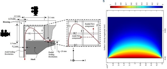
We start by summarizing the modeling approach by Baart et al. [11] as the numerical model is based on the same equations. Baart et al. [11] has used µPIV to measure the velocity profile across the grease pocket at a given plane set by the focal plane of the microscope. µPIV is a non-intrusive method that uses a high-speed camera connected to a microscope, and synchronized/triggered by a computer, to take images of a particle seeded (grease) flow; see, e.g., Green et al. [12] for further details. Through a correlation algorithm, the particle motion is tracked, and the velocity vectors in the geometry are obtained. In µPIV, the location of the measurements is set by the focal plane of the microscope, enabling measurements at different planes throughout a domain. For more details of the µPIV method the reader is referred to Raffel et al. [15]. Measuring the motion in the xr-plane, the camera is positioned to the left in Figure 1, and planes F1–3 represent possible locations of the actual plane. For a fully-transparent medium, the plane of measurement can be anywhere between F1 and F3 (and even closer to the boundaries). For greases, the possibility to measure deep into the flow is limited as the grease transparency is limited due to the thickener.
Baart et al. [11] used a correction factor (see below for more details) to account for the non-linearity in the flow due to the shear thinning rheology of the grease. The analytical model by Batchelor [13] is valid for the ideal flow case, i.e., a 1D flow where the ratio between the pocket gap and pocket length is <<1. For such a flow, the velocity profile is only dependent of the coordinate perpendicular to the gap (r-direction in Figure 1). The flow is driven by the rotating shaft (Figure 1). One of the benefits with the DRS geometry is that it enables a combined axial (leakage) flow; see Westerberg et al. [14], where the evolution of an introduced particle concentration is modeled. As the centrifugal force increases with a larger radius, a particle in the flow migrates to a larger radius, i.e., they travel in the positive radial direction from the rotating shaft. Baart et al. did not consider hydrodynamic effects due to shear, shear thinning, or normal stresses as discussed by e.g. Karnis and Mason [16]. The centrifugal force is written:
where a is the particle radius, ρp the particle density, ρg the grease density, the circumferential velocity and r the particle radial position (see Figure 1, Figure 2 and Figure 3). The drag force is described by the Stokes law:
where is the grease viscosity obtained from the four parameter Herschel-Bulkley model and is the particle velocity in the circumferential ϕ-direction. Table 1 summarizes the test particle migration parameters used by Baart et al. [11], and Table 2 summarizes the rheological parameters of the three greases used. Applying Newton’s second law for the forces and motion in the radial direction gives:
Here, mp is the particle mass and ar the particle acceleration. Considering the leakage flow velocity in the axial direction to be significantly lower than the velocity induced by the rotating axis, only the radial velocity component is considered. For the influence of a leakage flow on a contaminant particle concentration inserted into the domain, please see Westerberg et al. [14]. Further, the particle acceleration is set to zero as the grease viscosity is very high and the contaminant particles are very small, resulting in long migration times. Applying Equations (1) and (2) in Equation (3) and solving for the circumferential velocity component then yields:
In order to obtain the particle position as a function of time, Equation (4) was integrated numerically for a given time step (dt = 1 s) as the non-linear rheology of the grease does not enable an analytical solution. This forward integration method is called the Euler method and is the lowest order Runge–Kutta numerical scheme. This topic is discussed later on as it has particular relevance for the accuracy of the solution. is determined from an approach where the velocity profile for a Newtonian fluid between two circular cylinders [13] is combined with a correction term to account for the non-linearity in the flow due to the non-Newtonian rheology of the grease. The solution for the Newtonian flow reads.
where ri and ro are the inner and outer cylinders, respectively, and is the shaft speed. To obtain a solution for the non-Newtonian grease flow, Equation (5) has been modified such that:
where α is a fitting parameter and whose value is obtained from matching the expression for the velocity with measured velocity profiles using µPIV. For the case of an ideal 1D flow, there are no constraints in this approach as the flow velocity is solely dependent on the radial coordinate. As the velocity profile is measured in a plane located at a distinct location, this approach implies that the expression for the velocity given by Equation (6) is valid at the actual location of the measurement plane. However, at the same time, as the velocity profile is independent of the axial coordinate (i.e., the location of the measurement plane) for an ideal 1D flow, the obtained velocity profile is valid throughout the whole geometry, which for the actual case is comprised by the grease pocket; cf. location of planes F1–3 in Figure 1. The flow in the DRS grease pocket can be considered 1D when a ring is applied to reduce the gap in the radial direction (Figure 1) to 0.1 mm, compared to the distance between the boundaries in the axial (z) direction of 2 mm. For the case without ring, the situation is different as the length scales in both the z- and r-directions are of the same order. This implies that the boundaries with surface normal in the z-direction will influence the flow in the whole domain, and the velocity consequently also is a function of the z-coordinate.
2.2. Numerical Modeling of Particle Position in the Grease Pocket
In the numerical model, the exact same grease parameter values are used as in Baart et al. [11] in order to be able to conclude eventual differences in the migration results. Important to point out is that in reality, a difference in migration time can absolutely be due to the rheology of the grease or, more specifically, to local variations of the rheology due to the grease multiphase characteristics. It is not uncommon that lubricating greases experience local gradients of base oil or thickener concentration, causing effects such as shear banding in the bulk flow and slip effects in connection to solid boundaries. Both Baart et al.’s model and the present one however consider a single-phase grease, meaning the rheological properties of the grease are homogeneous throughout the grease pocket. As the same governing equations are used, with the exception of neglected acceleration by Baart et al., and the same rheology is used, eventual differences in migration results should reasonably be due to different numerical schemes used or limitations in the model(s), which do not enable one to fully resolve the physics in the flow.
Flow and Migration Model
Comsol Multiphysics v5.3 (denoted Comsol for simplicity) is used to simulate the results achieved on the narrow and the wide pockets. The analytical models presented by Baart et al. [11] do not consider the grease flow at the inlet at the radial sealing restriction (Figure 1), meaning they simplified one parameter of the experimental µPIV model presented by Green et al. [12]. It also means that a geometric simplification has been assumed for the pocket. The grease pocket flow modelled with Comsol has the same dimensions as the Baart et al. [11] model used for the grease particle migration without the radial and axial sealing restrictions (inlet and outlet). In the present model, the particle flow is affected by the centrifugal force (Fc.r) produced by the rotating shaft and the drag force (Fd.r) of the grease flow. Under these conditions, the particles experience forces in the radial (r) and tangential (z) directions as presented in Section 2.1.
The particle migration is modelled by first modelling the grease flow in the pocket. The flow model is built analogously to the flow model in Westerberg et al. [14]. Second, using the results from the grease flow model, a particle tracing model is used to include the particle’s drag force. To solve the laminar flow Comsol, use the equations for mass conservation (i.e., the continuity equation) and conservation of momentum, which for a stationary incompressible fluid read:
Here, η is the dynamic viscosity (which for the general case is a function of the shear rate; see Equation (11)), u the velocity, ρ the fluid density, p the pressure and I the identity matrix. The term in brackets multiplied with the viscosity is the general expression for the shear rate. For the particle migration model, the field variables change over time as the particle position does, meaning a time-dependent solver is chosen. Within the particle tracing module, the setting to include out-of-plane degrees of freedom is activated to consider the shaft rotation velocity on the particle model. The particle density and diameter are set according to the values in Table 1. As implemented in Comsol, the Stokes drag force law reads:
where v is the particle velocity, u the flow velocity and τ the particle velocity response (or relaxation) time:
Here, ρp is the particle density and dp the particle diameter. The right-hand side of Equation (9) can easily be shown to equal 6πηa(u − v) by expressing the mass using the density, a being the particle radius. This expression is perhaps better known as the Stokes law. In Comsol (Equation (9)), the centrifugal force is inherently considered, meaning the same governing equations are used as in Baart et al. [11] to describe the particle motion. The particle entrance flow is setup to inject one unique particle when the simulation starts. The initial radial position of the particle is at the rotating shaft (Figure 2), and the particle initial velocity is set from the module results of the grease flow model. The initial vertical position along the shaft boundary is varied depending on the case studied as shown later on in the paper. The housing wall has a frozen boundary condition, meaning the particle position and the velocity remain fixed once the particle has made contact with the housing.
The meshes used are Comsol’s automatically generated extremely fine meshes, controlled by the actual model physics. The DRS domain has a total of 230,416 and 33,966 elements for the wide and narrow pocket, respectively. Considering the symmetry in the DRS geometry, the domain is modelled using the 2D axisymmetric component in Comsol. The equations are solved using a single phase laminar flow model with a PARIDOS solver. As field variables do not change over time, a stationary solver is chosen. The laminar flow model is set up using an incompressible flow model without turbulence. The shaft rotation component velocity is considered through the variable uphi, which activates the Comsol swirl flow option. The fluid is described as a single-phase four-parameter Herschel–Bulkley (H-B) fluid with the density and rheological parameters presented in Table 2. The H-B model is considered as it is used in the model by Baart et al. [11]. Comsol enables a user-defined dynamic viscosity using the built-in variable spf.sr representing the shear rate in the flow. In terms of the dynamic viscosity, the four-parameter Herschel–Bulkley rheology model reads η = τy/γ + K∙γn−1 + ηbo, where τy is the yield stress value, γ the shear rate, K the grease consistency, n the shear thinning (n < 1) (or thickening, n > 1) parameter and ηbo the base oil viscosity. The values for these parameters are presented in Table 2. When modelling the flow numerically, the yield stress is a specific problem, as in the H-B model, it implies that the grease starts to deform (flow) when the shear stress in the flow is greater than the yield stress value; i.e., it is a discontinuous transition from not moving to moving grease. Numerically, we need to describe the transition in order for it to be continuous. Another numerical problem may arise in the limit of very small shear rates as the denominator in the expression for the H-B model will be very small, leading to convergence problems. The expression for the dynamic viscosity has then been described as (recalling that in Comsol spf.sr is the built-in shear rate value):
where f(spf.sr) = max(spf.sr, 0.0001) is a max-function returning the maximum value of the two arguments, i.e., if spf.sr (the shear rate) is greater than 0.0001, the actual value of spf.sr is returned. Otherwise, if spf.sr is smaller than 0.0001, the value 0.0001 will be returned. η is used to denote the dynamic viscosity in order to be consistent with previous notation, even though µ is used for the dynamic viscosity in Comsol. The term in the brackets multiplied with the yield stress serves to treat the transition from fully stationary grease to yielded grease. As shown in Figure 2, the shaft rotation is set up as a moving wall selecting the swirl flow option, which enables the velocity component in the azimuthal direction (uphi) to represent the shaft velocity . The housing pocket walls are set up with a no slip boundary condition. For avoiding singularities, a pressure point constraint of 0 Pa at the edge (corners in the axisymmetric geometry) of the housing wall is also set.
3. Results and Discussion
3.1. Velocity Field and Velocity Profiles in the Wide and Narrow Grease Pocket
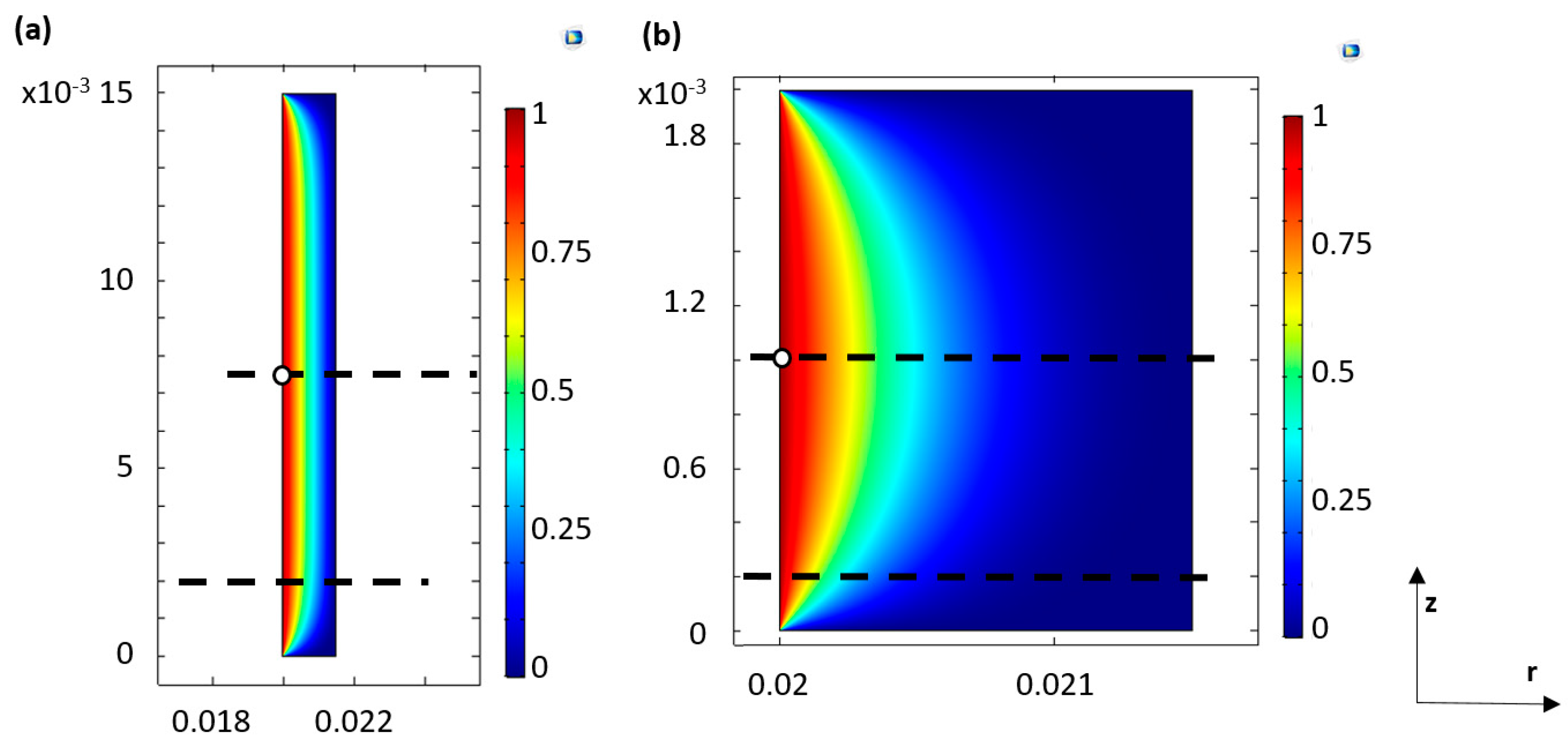
Modeling the particle migration, the first part is comprised of modeling the velocity field in the grease pocket. This flow field is then used by the particle migration module to calculate the forces acting on the particle. The velocity field magnitude distribution in the wide and narrow pocket is shown in Figure 3. Both pockets have the same width (distance between the rotating shaft and stationary housing); the wide grease pocket case (3a) has been modelled with the distance between the lateral walls (top and bottom boundaries) being 10-times the radial gap. This is to represent a 1D flow where the influence of the lateral walls is neglected. From the velocity distribution, it follows that the velocity is independent of the z-coordinate in the wide pocket, while the velocity is dependent on both r and z in the narrow pocket. This will have an impact on the particle migration time, as will be shown in the next subsection.
3.2. Particle Migration in the Wide Grease Pocket
The particle motion in the grease pocket is calculated by using the Comsol particle tracing module. The procedure is to first model with the Comsol laminar flow module the geometry and solve with the stationary solver to achieve the velocity field, as done in the previous paragraph. Then, from a given start position for a particle with a given density and radius (a spherical shape is assumed), the acting forces by means of the drag force and centrifugal force are calculated using the Comsol particle tracing module with a time-dependent solver. The time-dependent solver uses as the input value the velocity profile calculated at the stationary velocity field to calculate the dynamic viscosity due to the shear forces caused by the rotating shaft and then the drag force at the particle to obtain the particle position. Comsol uses a higher order Runge–Kutta algorithm for time integration, meaning the time step is set by the solver. Hence, the time step between iterations used by the time-dependent solver for the particle tracing simulations is dependent on the flow characteristics. This is highly important when discussing the results from the comparison with Baart et al. [11] later on as they used the Euler method, i.e., lowest order Runge–Kutta scheme, with a time step of 1 s when numerically integrating the particle velocity. Reconnecting to the Introduction, the numerical approach is also of specific interest in order to investigate its influence on the solution.
Figure 3a shows the initial position of the particle, placed at the left boundary (rotating shaft) and vertically halfway between the stationary lateral boundaries. This is to avoid the influence of the lateral walls in order to compare with the results by Baart et al. [11] who assume an ideal 1D flow for the wide pocket case. Figure 5 shows the results of the particle position in the radial direction over time in the wide channel compared with the corresponding results from the migration model by Baart et al. [11]. As shown, there is a phase shift (offset) between the two models, which correspond to a total deviation in migration time of 16%. In order to investigate the reason for this deviation, we recall that the rheology model used has been validated by Westerberg et al. [14]. Further, there is no difference for the case of a wider pocket; this is also supported by the velocity field in Figure 3 showing a homogeneous velocity distribution except for close to the boundaries. It is hence reasonable to assume that other physical properties of the flow affect the solutions and which effects have not been captured by the approach used by Baart et al. [11]. For instance, as presented earlier, Baart et al. [11] have neglected the acceleration of the particle, and they also have used the straightforward Euler method of integrating the particle position considering a fixed time step of 1 s. The Euler method is also the lowest order Runge–Kutta method. Runge–Kutta methods comprise a family of numerical methods which approximate solutions to ordinary differential equations (ODEs).
For a more in-depth coverage of numerical methods and details on the Runge–Kutta methods, the reader is referred to books on numerical analysis, e.g., Moin [17], which has an engineering approach. To zoom in on the most relevant parts for the present flows scenarios, we consider the time step error, which is a product of the error coefficient, and the time step to a certain power, which denotes the order of the method. The Euler method is of order one. The difference between a higher order method and the Euler method is that the time step error decreases, consequently increasing the accuracy of the model. Moin [17] compares the analytical solution of an oscillating spring, which initially has been subjected to a certain displacement causing an oscillation around the equilibrium position. It follows that the Euler method does not fully capture the dynamics of the solution, showing both a phase shift and a lower amplitude. It requires a Runge–Kutta method of order four to obtain an approximate solution that fits the analytical solution. Putting this into the context of the present flow and calculation of the particle position, the first order Runge–Kutta method does not capture the dynamics of the particle in the grease flow, resulting in the phase shift observed in Figure 5. Investigating the velocity evolution, the numerical model reveals that the particle experiences an acceleration peak the first 10 seconds; this is of course not captured by the analytical model neglecting the acceleration. Furthermore, rapid changes are not captured by applying the Euler method. The rapid changes appear in connection with the rotating shaft where the particle is inserted into the flow, the centrifugal forces are largest and the particle undergoes a change (acceleration) from stationary to moving with the flow. Altogether, it can be concluded that the improved accuracy of the higher (fourth) order Runge–Kutta method compared to the Euler method is mirrored by the faster migration time.
3.3. Particle Migration in the Narrow Grease Pocket
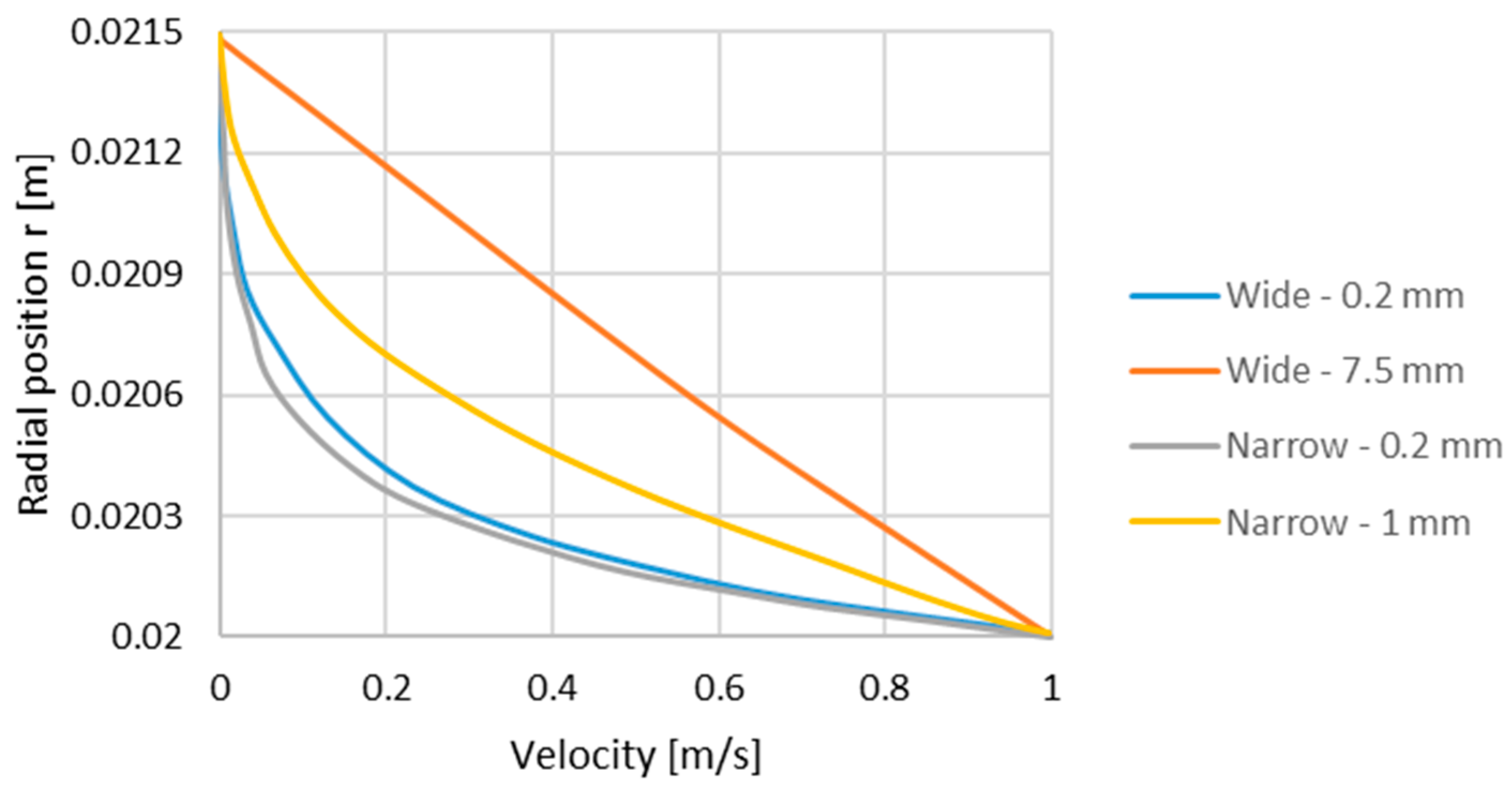
Figure 6 shows the results of particle migration in the narrow grease pocket. Comparing with the results by Baart et al. [11], the numerical model shows a significantly shorter migration time. Comparing with the migration time in the wide pocket, it follows that the numerical model indicates a shorter migration time in the narrow pocket, while the model by Baart et al. [11] indicates a longer migration time in the narrow pocket compared to in the wide pocket. There hence is a difference between the two models for a given pocket size, but also how the migration time changes between different pocket sizes. Here, we recall that the actual migration considered is for the radial direction from the rotating shaft to the (in the radial direction opposite located) stationary housing. The radial distance for the particle to travel is also the same for both grease pockets. To unravel the mechanisms behind these observations, we start by comparing the difference in migration time between the grease pocket sizes as modeled by Baart et al. [11]. From Figure 5 and Figure 6, it follows that the migration time is longer in the narrow pocket. This result is directly mirrored by the orange and grey velocity profiles in Figure 4, which are used in the calculation of the particle velocity. For the wide pocket inheriting a 1D flow independent of the gradients induced by the lateral walls, the orange velocity profile represents the profile in the pocket. The grey velocity profile is the corresponding profile in the narrow pocket used in the modeling work. The orange profile equals the analytical solution by Batchelor (Equation (5)), and the grey velocity profile is the one from which the α-value used in Equation (6) is calculated. The α-value is used in the exponential function, which is used to account for the non-linearity in the flow due to the shear thinning rheology of the grease. Baart et al. [11] used velocity profiles from µPIV measurements; the grey velocity profile in Figure 4 in Westerberg et al. [14] has been validated with µPIV data for the NLGI2 grease, meaning they are considered equal. The straightforward explanation for the faster migration time in the wide pocket is that the particle gas exhibited a higher velocity throughout the gap (cf. the orange and grey velocity profiles). For both the wide and narrow pocket, the velocity field is by Baart et al. [11] assumed 1D in the sense that u = uϕ(r)aϕ, where aϕ is the unit vector in the circumferential direction. This is in every aspect correct for the wide channel (ideal 1D flow) as the lateral boundaries will not influence the flow, and hence, the velocity field only has one component (ϕ), which is only dependent on the radial coordinate. The µPIV measurements used for the wide pocket migration modeling enable measurements of the velocity at a plane determined by the focal plane of the microscope. This means that the motion/flow in and out of the plane is not captured, which in turn yields that the velocity profile used in the migration model by Baart et al. [11] for the wide channel implies a migration model valid in this particular plane; physically, this can be viewed as the radial component contribution to the migration. Important to point out is that this indeed is a valid and relevant model, but it can be considered as a lowest order solution, as the full velocity field is not solved, meaning the contribution from components other than the radial component are not included. Continuing with the migration results from the numerical model, it is clear that in the narrow pocket, the migration time is several orders of magnitude smaller than in the wide pocket. Reconnecting to the velocity profile in the narrow pocket versus the corresponding profile in the wide pocket (Figure 4), it may seem contradictory with a faster migration in the narrow pocket as the velocity is lower. However, the velocity profiles in Figure 4 are valid for the location of the actual plane as denoted in the figure (dashed red line in Figure 3); i.e., the vertical distance from the lateral wall. With gradients in the flow in other spatial directions, the particle will be subject to a flow field dependent also on the z-coordinate, inducing drag force components in other directions than the radial direction. In Figure 7, the particle positions (r- and z-components) for different start positions in the wide pocket are shown. Interestingly, for other vertical start positions than between the lateral walls (F2 = 1 mm; F2 represents the plane for which the µPIV measurements have been made), the particle does not reach the stationary housing before hitting the lateral wall as shown by the z-coordinate of the particle. Additionally, with a no-slip boundary condition (u = 0), the particle is stuck at the lateral wall once reaching it. Gradients in the flow induced by the lateral walls can hence be concluded to influence the particle migration except at the mid-plane between the lateral boundaries (z = 1 mm). With a parabolic velocity distribution (Figure 4), the maximum velocity is at the mid-plane between the lateral walls, and with that start position being the only position from which the particle manages to reach the stationary housing, it can be argued that that is the reason for the shorter migration time in the narrow pocket compared to the results by Baart et al. [11]. Furthermore, the velocity profile from µPIV measurements used by Baart et al. cannot be from a plane as far into the flow as 1 mm due to the limited transparency of the grease. According to Baart et al., the location of the plane is approximately 0.2 mm from the lateral wall, represented by the transparent window in the DRS geometry. This supports the observation of a longer migration time from the model by Baart et al. as the velocity is significantly lower, so close to the lateral boundary as 0.2 mm. As shown in Figure 7, the trend is clear with the particle hitting the lateral wall earlier as the initial distance from the lateral wall decreases. Relating this to the model by Baart et al., their model indeed is relevant for comparisons with the numerical results, as the physics close to the wall is not resolved in the numerical model. There, the rheology of the grease is assumed to be homogeneous throughout the whole grease pocket. However, as shown, e.g., by Westerberg et al. [4], there is a heterogeneous region present close to the solid boundaries where the shear rate is high, enabling particle migration due to, e.g., wall slip or shear banding caused by a locally different grease rheology and phase composition.
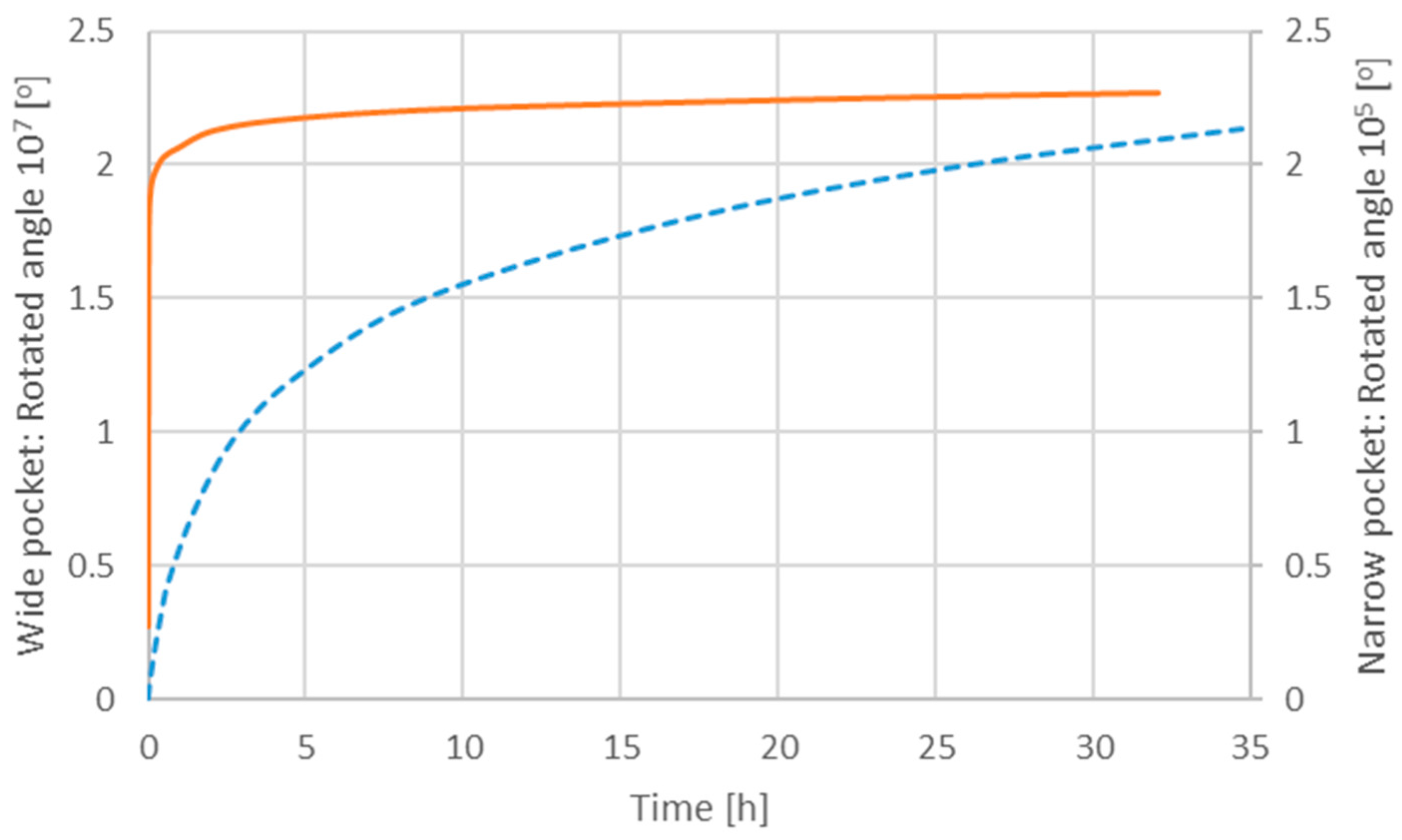
Going back to the seemingly strange numerical result of shorter migration time in the narrow pocket compared to the wide pocket, Figure 8 shows the number of degrees in the ϕ-direction the particle travels with time. From these plots, we see that in the wide pocket, the rotated angle is much greater than in the narrow pocket (note the different scale). In the narrow pocket, the particle reaches its maximum angle rotated after the time elapsed for migrating the full radial distance to the stationary housing (cf. Figure 6). Comparing with the degrees rotated in the wide channel, during the same time lapse, the particle rotation angle in the wide pocket is approximately a factor 50 larger compared to the rotation angle in the narrow pocket. Recalling that the rotating shaft has the same speed (1 m/s) in both cases, the reason for the faster rotation in the wide pocket must lie in the geometry of the pocket, which in turn yields a different shear rate. However, with the same distance between the rotating shaft and the stationary housing in both the wide and narrow pocket, the change in flow dynamics due to the lateral walls is then arguably the reason for the difference in migration time. The narrow pocket can be viewed as the merged ideal 1D cases comprised by the present wide pocket where the distance between the lateral walls is much greater than the distance between the shaft and housing and the opposite 1D case where the distance between the lateral walls are as in the present narrow pocket, while the distance between the shaft and housing is much greater. For the latter case, there is a contribution from the lateral boundaries to the shear rate equaling , in addition to the shear rate in the wide pocket case equaling . The net shear rate in the narrow pocket then reads . The increased shear motion in the circumferential direction induces the increased rotation in the narrow pocket, which in turn increases the centrifugal force on the particle, consequently speeding up the migration. Furthermore, as the grease is shear thinning, an increased shear rate yields a lower viscosity, which in turn yields a reduced drag on the particle.
4. Summary and Conclusions
In this study, the commercial software Comsol Multiphysics v.5.3 is used to numerically model particle migration in a grease pocket where the flow is driven by a rotating shaft. The model uses the same rheology as in Baart et al. [11], and the results obtained have been compared with their model results. The main differences between the two models are that the numerical model uses a higher order numerical scheme to solve the particle position as function of time and that the full 3D flow in the pocket is modelled, which results in all forces acting on the particle, compared to Baart et al. [11], who solely investigate the contribution from the radial component.
It was found that for a one-dimensional pocket flow, the two migration models differ solely by means of a phase shift (offset), with a faster migration time observed for the numerical model. This result is argued to be due to the numerical methods used, with the lowest order Runge–Kutta method used by Baart et al. [11] having limited accuracy solving the temporal behavior compared to the higher order method used in the numerical model. For the flow in a pocket geometry where the distance between the lateral boundaries, which in the previous case is much greater than the distance between the rotating shaft driving the flow and in the radial direction opposite the stationary housing, is of the same order as the distance between the shaft and housing, there is a great difference in migration time between the two models with the numerical model showing a significantly faster migration time. In addition to the effects from the numerical solver as previously addressed, the geometry of the grease pocket holds the secret of the faster migration. The lateral walls induce gradients in the flow, causing the shear rate in the pocket to increase and, as a consequence, a faster motion in the azimuthal direction. This in turn yields increased centrifugal force acting on the particle, leading to a stronger driving force in the radial direction and ultimately a faster particle transport in the pocket.
Acknowledgments
This project is part of Smart Machines and Material (SM2) at Luleå University of Technology (LTU). Laulagun Bearings, S. L. is gratefully acknowledged for fruitful discussions.
Author Contributions
The numerical simulations were conducted by Josep Farré-Lladós and Chiranjit Sarkar. Jasmina Casals-Terré and Lars-Göran Westerberg provided technical and scientific guidance to the computational work. Lars-Göran Westerberg wrote the paper.
Conflicts of Interest
The authors declare no conflict of interest.
References
- Lugt, P.M. Grease Lubrication in Rolling Bearings; Wiley: Hoboken, NJ, USA, 2013; ISBN 978-1-118-35391-2. [Google Scholar]
- Torbacke, M.; Rudolphi, A.K.; Kassfeldt, E. Lubricants Properties and Performance; Luleå Tekniska Universitet: Luleå, Sweden, 2012; ISBN 978-91-7439-410-8. [Google Scholar]
- Rizvi, S.Q.A. A Comprehensive Review of Lubricant Chemestry, Technology, Selection and Design; ASTM International: Conshohocken, PA, USA, 2009; ISBN 978-0-8031-7000-1. [Google Scholar]
- Westerberg, L.G.; Lundström, T.S.; Höglund, E.; Lugt, P.M. Investigation of Grease Flow in a Rectangular Channel Including Wall Slip Effects Using Microparticle Image. Tribol. Trans. 2010, 53, 600–609. [Google Scholar] [CrossRef]
- Li, J.X.; Höglund, E.; Westerberg, L.G.; Green, T.M.; Lundström, T.S.; Lugt, P.M.; Baart, P. μpIV measurement of grease velocity profiles in channels with two different types of flow restrictions. Tribol. Int. 2012, 54, 94–99. [Google Scholar] [CrossRef]
- Tallian, T.E. Failure Atlas for Hertz Contact Machine Elements, 2nd ed.; ASME Press: New York, NY, USA, 1999; ISBN 0-7918-0084-9. [Google Scholar]
- Farré-Lladós, J.; Westerberg, L.G.; Casals-Terré, J. New method for lubricating wind turbine pitch gears using embedded micro-nozzles. J. Mech. Sci. Technol. 2017, 31, 797–806. [Google Scholar] [CrossRef]
- Strubel, V.; Simoens, S.; Vergne, P.; Fillot, N.; Ville, F.; El Hajem, M.; Devaux, N.; Mondelin, A.; Maheo, Y. Fluorescence Tracking and µ-PIV of Individual Particles and Lubricant Flow in and around Lubricated Point Contacts. Tribol. Lett. 2017, 65, 75. [Google Scholar] [CrossRef]
- Tropea, C.; Yarin, A.L.; Foss, J.F. Handbook of Experimental Fluid Mechanics; Springer: Berlin, Germany, 2007; ISBN 978-3-540-25141-5. [Google Scholar]
- Franken, M.J.Z.; Chennaoui, M.; Wang, J. Mapping of Grease Migration in High-Speed Bearings Using a Technique Based on Fluorescence Spectroscopy. Tribol. Trans. 2017, 60, 789–793. [Google Scholar] [CrossRef]
- Baart, P.; Green, T.M.; Li, J.X.; Lundström, T.S.; Westerberg, L.G.; Höglund, E.; Lugt, P.M. The Influence of Speed, Grease Type, and Temperature on Radial Contaminant Particle Migration in a Double Restriction Seal. Tribol. Trans. 2011, 54, 867–877. [Google Scholar] [CrossRef]
- Green, T.M.; Baart, P.; Westerberg, L.G.; Lundström, T.S.; Höglund, E.; Lugt, P.M.; Li, J.X. A New Method to Visualize Grease Flow in a Double Restriction Seal Using Microparticle Image Velocimetry. Tribol. Trans. 2011, 54, 784–792. [Google Scholar] [CrossRef]
- Batchelor, G.K. An Introduction to Fluid Dynamics; Cambridge University Press: New York, NY, USA, 2009. [Google Scholar]
- Westerberg, L.G.; Sarkar, C.; Farre, J.; Lundstrom, T.S. Lubricating Grease Flow in a Double Restriction Seal Geometry: A Computational Fluid Dynamics Approach. Tribol. Lett. 2017, 65, 1–17. [Google Scholar] [CrossRef]
- Raffel, M.; Willert, C.E.; Wereley, S.; Kompenhans, J. Particle Image Velocimetry, 2nd ed.; Springer: Berlin, Germany, 2007. [Google Scholar]
- Karnis, A.; Mason, S.G. Particle Motions in Sheared Suspensions. XIX. Viscoelastic Media. J. Rheol. 1966, 10, 571–592. [Google Scholar] [CrossRef]
- Moin, P. Fundamentals of Engineering Numerical Analysis; Cambridge University Press: Cambridge, UK, 2010; ISBN 9780511781438. [Google Scholar]
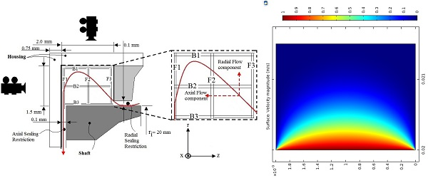
Figure 1.
Schematic of the DRS geometry developed by Green et al. [12] to visualize velocity profiles in the grease pocket using micro Particle Image Velocimetry (µPIV). The setup enables measurements of the three flow components. F1–3 and B1–3 symbolize possible measurement planes. The thick red arrow indicates the direction of the leakage particle motion [14] (not covered in the present study), while the dashed black line is the rotating shaft, and the solid black lines are the stationary housing. The solid black lines also denote the lateral boundaries.
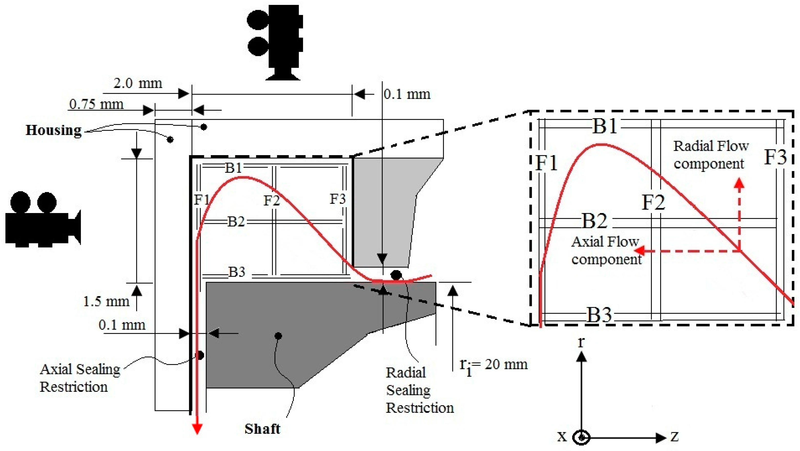
Figure 2.
Comsol 2D axisymmetric geometry model of the narrow pocket. The blue boundaries represent the stationary boundaries.
Figure 2.
Comsol 2D axisymmetric geometry model of the narrow pocket. The blue boundaries represent the stationary boundaries.
Figure 3.
NLGI2 grease velocity field, wide pocket (a) and narrow pocket (b). The red dashed lines illustrate the planes at which the velocity profiles in Figure 4 are. The white dot is the starting position for the particle in the migration simulation.
Figure 3.
NLGI2 grease velocity field, wide pocket (a) and narrow pocket (b). The red dashed lines illustrate the planes at which the velocity profiles in Figure 4 are. The white dot is the starting position for the particle in the migration simulation.

Figure 4.
NLGI2 grease velocity profile for the narrow and wide pocket with a shaft speed velocity of 1 m/s. The velocity profiles for the narrow pocket (positions 0.2 mm and 1 mm) were also validated by Westerberg et al. [14].
Figure 4.
NLGI2 grease velocity profile for the narrow and wide pocket with a shaft speed velocity of 1 m/s. The velocity profiles for the narrow pocket (positions 0.2 mm and 1 mm) were also validated by Westerberg et al. [14].

Figure 5.
Particle migration in the NLGI00, NLGI1 and NLGI2 greases. The dashed lines are the results from Baart et al.’s model [11] and the solid lines the numerical results. The initial position for the particle for the numerical model is shown by the white dot in Figure 3b. Blue: NLGI2, black: NLGI1, and red: NLGI00.
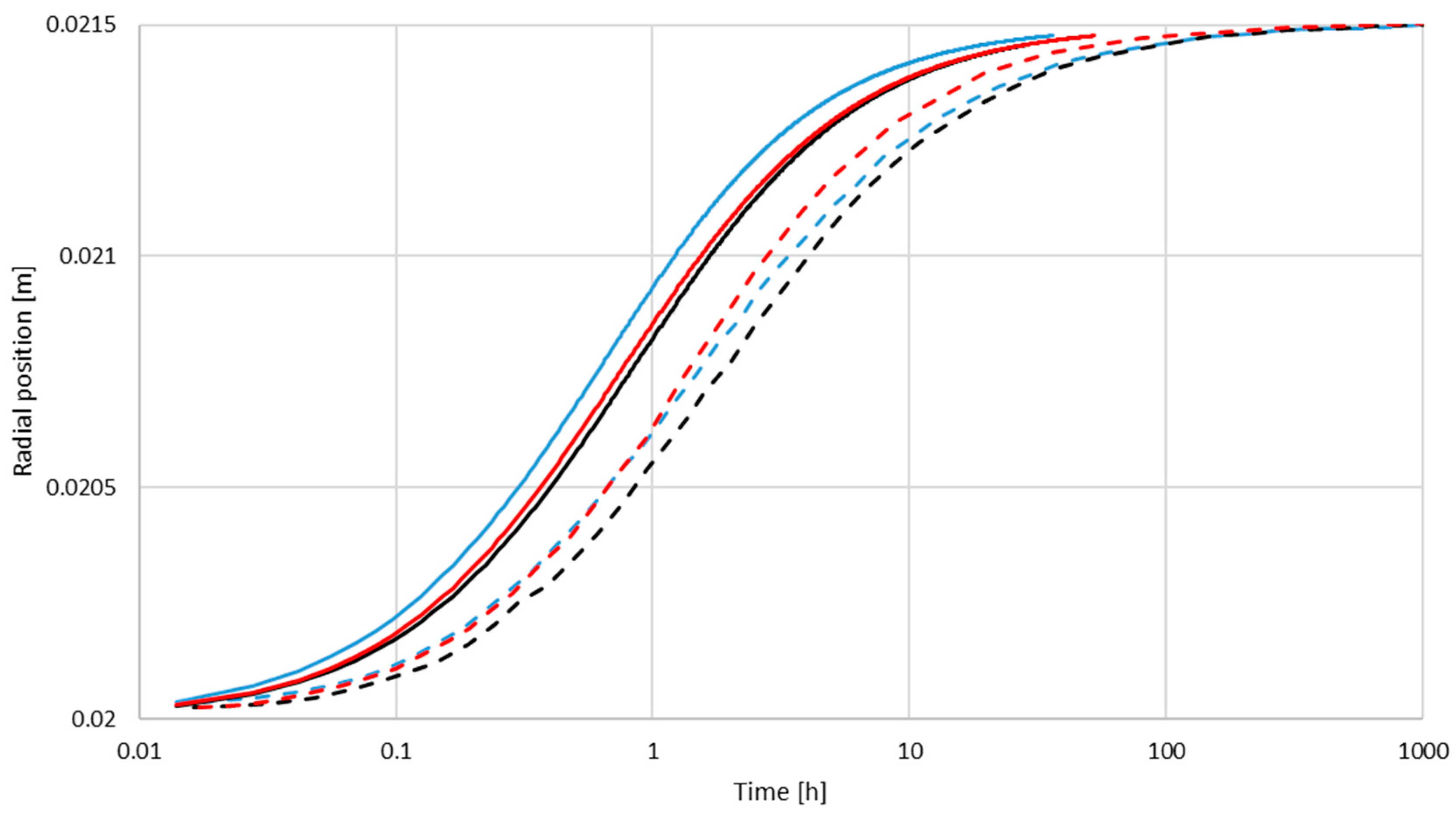
Figure 6.
Particle migration of the three greases. Numerical model results (solid lines) and Baart et al.’s results [11] (dashed lines). The initial position for the particle for the numerical model is shown by the white dotted in Figure 3b. Blue: NLGI2, black: NLGI1, and red: NLGI00.
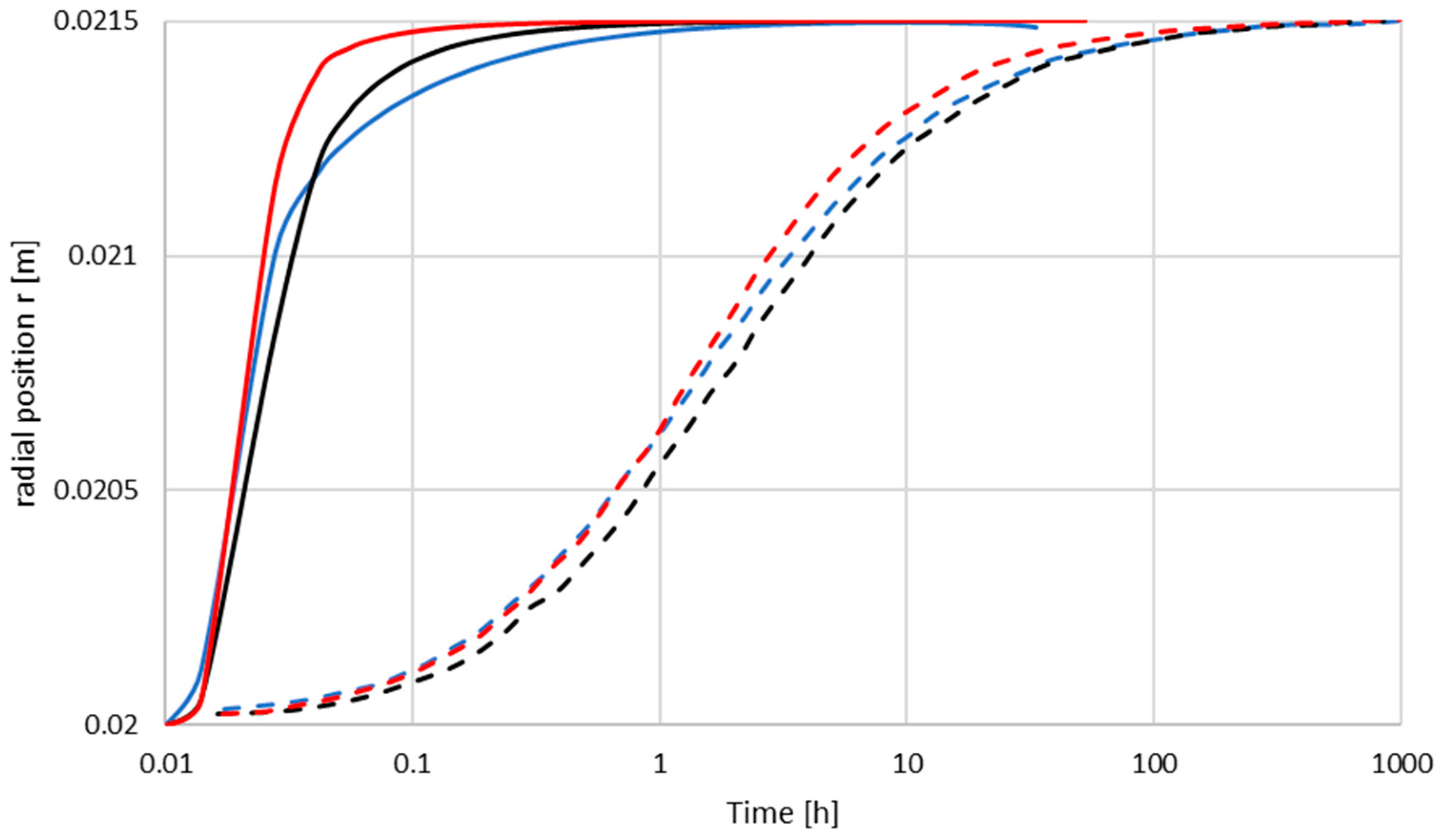
Figure 7.
Particle motion of the NLGI2 grease (r- and z-components) in the narrow grease pocket for different start locations along the rotating shaft, calculated from the lateral boundary. One millimeter equals a start position at the mid-plane between the two lateral boundaries.
Figure 7.
Particle motion of the NLGI2 grease (r- and z-components) in the narrow grease pocket for different start locations along the rotating shaft, calculated from the lateral boundary. One millimeter equals a start position at the mid-plane between the two lateral boundaries.
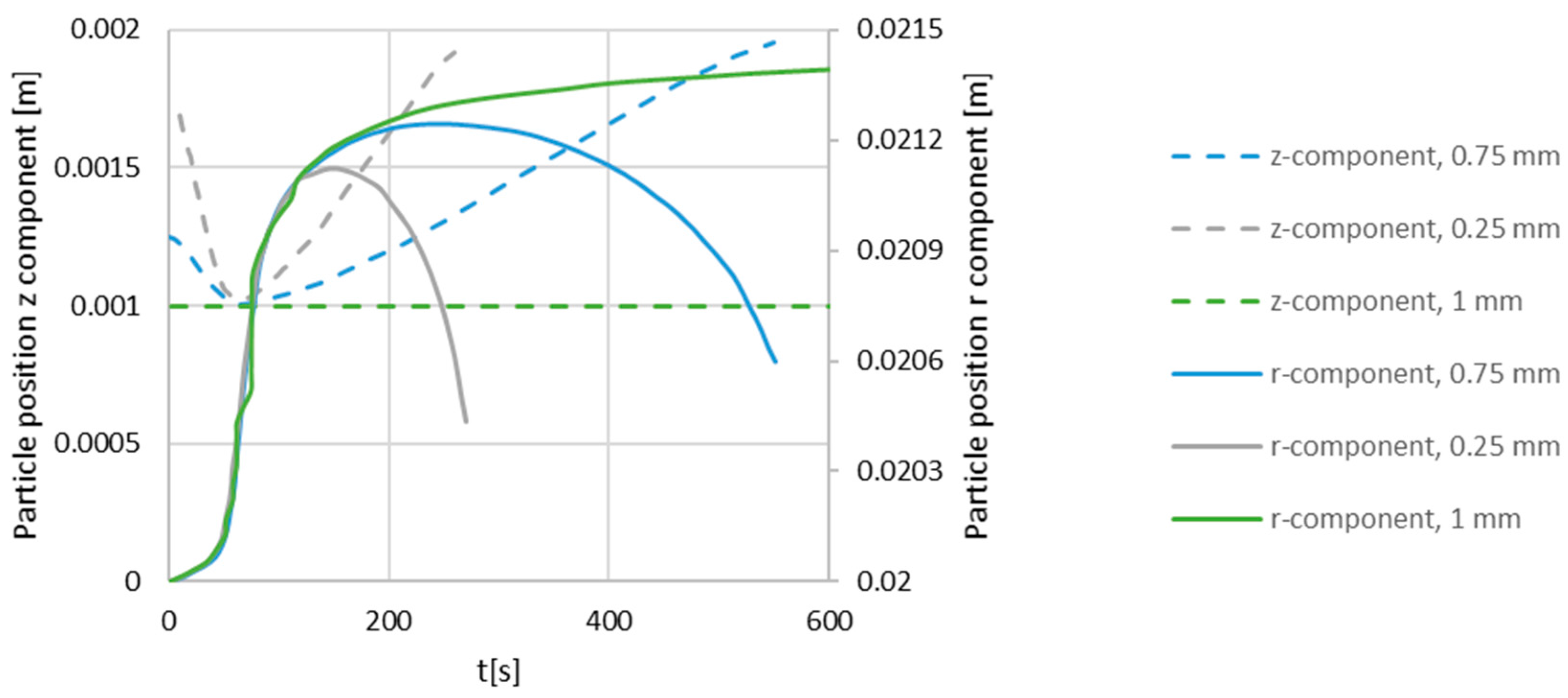
Figure 8.
Number of particle revolutions (in degrees) due to the circumferential velocity as a function of time (hours). Dashed line: wide pocket. Solid line: narrow pocket.
Figure 8.
Number of particle revolutions (in degrees) due to the circumferential velocity as a function of time (hours). Dashed line: wide pocket. Solid line: narrow pocket.

Table 1.
Test parameters from Baart et al. [11].
Table 1.
Test parameters from Baart et al. [11].
| a (µm) | ρp (kg/m3) | (m/s) | Temperature Test (°C) |
|---|---|---|---|
| 7 | 2100 | 1 | 25 |
Table 2.
Grease rheological parameters based on the three-parameter Herschel–Bulkley rheological model. From Baart et al. [11]. The parameters are (from left to right): the yield stress, grease consistency, shear thinning exponent, base oil viscosity and density. α is the fitting parameter in Equation (6).
| NLGI 1 grade | τyield (Pa) | K (Pa.s) | n | ƞbo (Pa.s) | ρg (kg/m3) | α (m−1) |
|---|---|---|---|---|---|---|
| 00 | 15 | 12 | 0.63 | 0.89 | 890 | −1000 |
| 1 | 260 | 61 | 0.42 | 0.49 | 910 | −2000 |
| 2 | 500 | 8.2 | 0.63 | 0.25 | 930 | −3000 |
1 The National Lubricating Grease Institute.
© 2018 by the authors. Licensee MDPI, Basel, Switzerland. This article is an open access article distributed under the terms and conditions of the Creative Commons Attribution (CC BY) license (http://creativecommons.org/licenses/by/4.0/).
Share and Cite
MDPI and ACS Style
Westerberg, L.-G.; Farré-Lladós, J.; Sarkar, C.; Casals-Terré, J. Contaminant Particle Motion in Lubricating Grease Flow: A Computational Fluid Dynamics Approach. Lubricants 2018, 6, 10. https://doi.org/10.3390/lubricants6010010
AMA Style
Westerberg L-G, Farré-Lladós J, Sarkar C, Casals-Terré J. Contaminant Particle Motion in Lubricating Grease Flow: A Computational Fluid Dynamics Approach. Lubricants. 2018; 6(1):10. https://doi.org/10.3390/lubricants6010010
Chicago/Turabian StyleWesterberg, Lars-Göran, Josep Farré-Lladós, Chiranjit Sarkar, and Jasmina Casals-Terré. 2018. "Contaminant Particle Motion in Lubricating Grease Flow: A Computational Fluid Dynamics Approach" Lubricants 6, no. 1: 10. https://doi.org/10.3390/lubricants6010010
Note that from the first issue of 2016, this journal uses article numbers instead of page numbers. See further details here.