Thermo-Hydrodynamic Analysis of a Plain Journal Bearing on the Basis of a New Mass Conserving Cavitation Algorithm

Abstract

Accurate prediction of cavitation is an important feature in hydrodynamic bearing modeling. Especially for thermo-hydrodynamic modeling, it is crucial to use a mass-conservative cavitation algorithm. This paper introduces a new mass-conserving Reynolds cavitation algorithm, which provides fast convergence and easy implementation in finite element models. The proposed algorithm is based on a variable transformation for both the pressure and mass fraction, which is presented in the form of a complementary condition. Stabilization in the streamline and crosswind direction is provided by artificial diffusion. The model is completed by including a simple and efficient thermal model and is validated using the numerical values of a reference plain journal bearing experiment under steady-state conditions. In addition, a transient analysis is performed of a journal bearing subjected to a harmonic load. It is shown that the proposed cavitation algorithm results are in good agreement with the reference measurement results. Moreover, the algorithm proves to be stable and requires only a small number of iterations to convergence in the Reynolds-based finite element model.

1. Introduction

Hydrodynamic bearings are machine elements used for separating moving components that have a relative velocity. In these bearings, the relative sliding velocity of the surfaces that border the fluid film causes a shear flow in the fluid. When this flow enters a converging volume, the pressure increases, which explains the carrying capacity of the bearing. Accurate predictions of this carrying capacity are crucial for an accurate design and, thus, for preventing any unwanted contact that can result in noise, wear, excessive friction or even failure of the bearing [1].

The commonly-used mathematical description of the pressure distribution in a hydrodynamic bearing is the classical Reynolds equation. Solutions of the Reynolds equation can contain negative pressures for flow through diverging sections or for the normal motion of walls moving apart. Fluids, however, can only hold a very limited amount of tensile stress before film rupture occurs [2]. This cavitation thus needs to be included in the bearing modeling. Numerous methods have been proposed for this purpose, as summarized in the review papers of Dowson and Braun [2,3].

In many of the early approaches, such as the Sommerfeld, the Gümbel "half-Sommerfeld" and the Swift and Stieber Reynolds approach, conservation of mass throughout the fluid and cavitation domain is not considered [3]. This shortcoming might sometimes only slightly affect the bearing reaction forces; conservation of mass is, however, an important condition for models that should include thermal modeling [4] or for models that treat surface texture, especially if accurate friction losses are to be calculated [5,6].

A popular cavitation algorithm nowadays was proposed by Elrod [7], who developed a method in which a switch function is used, automatically satisfying the boundary conditions at the cavitation interfaces, and which is based on the mass-conservative boundary conditions formulated by Floberg, Jakobson and Olsson [8]. Brewe [9,10] found excellent agreement with Jakobson’s experimental data for dynamically loaded bearings using Elrod’s algorithm.

Cavitation algorithms based on a finite element formulation are compared in Bayada et al. [11]. Many of these algorithms are presented in the form of a complimentary condition, i.e., in the cavitated regions, the mass fraction distribution is unknown, and the pressure distribution is known, whereas in the full film region, the pressure distribution is unknown, and the mass fraction distribution is known.

In the proposed algorithm in this paper, the same logic has been implemented, based on a variable transformation where both the mass fraction f and the pressure p are replaced by known functions of a new variable ξ. Thus, the modified Reynolds equation can be solved for this variable, and the pressure and mass fraction distribution can be obtained from the inverse transformation functions. The proposed mass-conserving cavitation algorithm is developed and used in a general purpose finite element code [12], which allows for the formulation of problems as a set of strongly coupled non-linear partial differential equations (PDEs). Moreover, it can be used in any finite element code that allows the arbitrary definition of the PDE coefficients and the solution of non-linear systems of equations using a simple fixed-point iteration.

In this paper, the cavitation algorithm is first applied on a 1D test problem, the infinitely long journal bearing, in order to demonstrate the streamline stabilization technique. Subsequently, the 1D stabilized model is expanded to a 2D finite journal bearing model in order to demonstrate the crosswind stabilization technique from which the complete stabilized 2D Reynolds equation is obtained. This model is then expanded to include a classic adiabatic thermal model, i.e., assuming adiabatic boundary conditions at the fluid-solid interfaces and assuming an effective temperature field across the film thickness (see, for instance, Pinkus [13]). These simplifications reduce the 3D heat transport model to a simple and efficient 2D model for the thin oil film. Subsequently, the 2D THD model is validated by a numerical case study of a finite length journal bearing under steady load conditions [14]. Finally, for the sake of completeness, a time transient analysis is performed using a dynamic load on the journal, after which the results are discussed.

2. Development of a New Mass-Conserving Reynolds Cavitation Algorithm

The distribution of pressure p and mass fraction f in a 2D lubricating film with film thickness h can be described using the Reynolds equation:

$$\frac{\partial }{\partial x}\left(-\frac{h^{3}f\rho }{12\eta }\frac{\partial p}{\partial x}+\frac{Uhf\rho }{2}\right)+\frac{\partial }{\partial y}\left(-\frac{h^{3}f\rho }{12\eta }\frac{\partial p}{\partial y}\right)+\frac{\partial hf\rho }{\partial t}=0$$

(1)

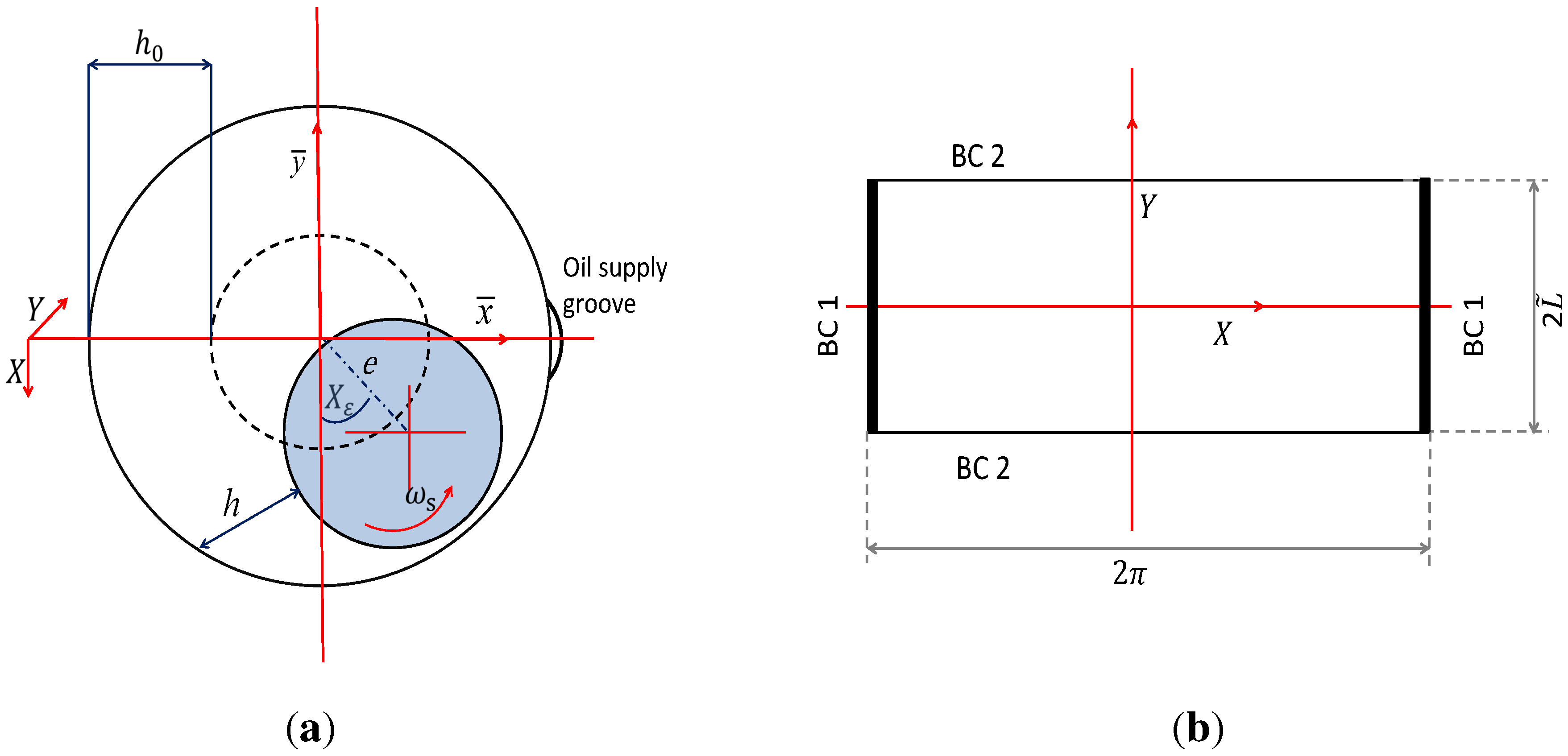
where $\eta ,\rho$ and U are the viscosity, density and surface velocity, respectively. x- and y-directions are in the direction of and perpendicular to the surface sliding velocity, respectively. It is assumed that only the shaft has velocity U in the x-direction; all other surfaces are stationary. Moreover, all surfaces are assumed to be rigid. As schematically depicted in Figure 1a, the attitude angle $X_{\epsilon }$ can be calculated as follows:

$$X_{\epsilon }=arctan\left(\frac{{\epsilon }_{\overline{y}}}{{\epsilon }_{\overline{x}}}\right)$$

(2)

where ε is the eccentricity ratio $(\epsilon =\frac{e}{h_0})$. $\overline{x}$ and $\overline{y}$ are the global coordinates with the origin in the center of the bearing. Assuming perfect alignment of the journal and taking into account the attitude angle $X_{\epsilon }$, the expression for the film thickness may be written as:

$$h=h_0(1-{\epsilon }_{\overline{x}}cos\left(x/R\right)-{\epsilon }_{\overline{y}}sin(x/R))$$

(3)

where $h_0$ is the nominal radial clearance. For the sake of numerical robustness, the problem is scaled using the following dimensionless variables:

$$\begin{array}{cccccccccc}\hfill P& =\frac{p{h}_0^2}{{\eta }_{0}UR}\hfill & \hfill W& =\frac{w{h}_0^2}{{\eta }_{0}U{R}^3}\hfill & \hfill \tilde{\rho }& =\frac{\rho }{{\rho }_0}\hfill & \hfill \tilde{\eta }& =\frac{\eta }{{\eta }_0}\hfill & \hfill X& =\frac{x}{R}\hfill \\ \hfill Y& =\frac{y}{R}\hfill & \hfill H& =\frac{h}{h_0}\hfill & \hfill \tilde{L}& =\frac{L}{R}\hfill & \hfill \tilde{t}& =t\omega \hfill \end{array}$$

(4)

which results in the following dimensionless Reynolds equation:

$$\frac{\partial }{\partial X}\left(-\frac{H^{3}f\tilde{\rho }}{12\tilde{\eta }}\frac{\partial P}{\partial X}+\frac{Hf\tilde{\rho }}{2}\right)+\frac{\partial }{\partial Y}\left(-\frac{H^{3}f\tilde{\rho }}{12\tilde{\eta }}\frac{\partial P}{\partial Y}\right)+\frac{\partial Hf\tilde{\rho }}{\partial \tilde{t}}=0$$

(5)

where the normalized film thickness is given by:

$$H=1-{\epsilon }_{\overline{x}}cos\left(X\right)-{\epsilon }_{\overline{y}}sin\left(X\right)$$

(6)

Note that the circumferential and axial flows, $q_X$ and $q_Y$, respectively, are represented by the terms between brackets $\left(\frac{\partial }{\partial X}\left(q_X\right)\mathrm{and}\frac{\partial }{\partial Y}\left(q_Y\right)\right)$ in Equation 5 and can thus simply be computed as follows:

$$\begin{array}{}\mathrm{(7a)}& \hfill q_X& =-\frac{H^{3}f\tilde{\rho }}{12\tilde{\eta }}\frac{\partial P}{\partial X}+\frac{Hf\tilde{\rho }}{2}\hfill \mathrm{(7b)}& \hfill q_Y& =-\frac{H^{3}f\tilde{\rho }}{12\tilde{\eta }}\frac{\partial P}{\partial Y}\hfill \end{array}$$

In Figure 1a,b, the kinematics of the plain journal bearing and the computational fluid domain with the imposed boundary conditions are presented, respectively. The supply groove is positioned at $X=-\pi ,X=\pi$, over the full width of the bearing. The specific boundary conditions (BCs) for the 1D and 2D case will be defined in each section. In Figure 1, the X-and Y-directions are in the direction of and perpendicular to the surface sliding velocity, respectively.

Figure 1. Bearing configuration: (a) kinematics of the plain journal bearing (dimensions are exaggerated) with eccentricity amplitude e; (b) fluid domain of the plain journal bearing with applied boundary conditions $BC$.

Figure 1. Bearing configuration: (a) kinematics of the plain journal bearing (dimensions are exaggerated) with eccentricity amplitude e; (b) fluid domain of the plain journal bearing with applied boundary conditions $BC$.

For most practical applications where the hydrodynamic pressure will increase to values much higher than the cavitation pressure, it may be assumed that the cavitation pressure is equal to zero. With this simplification, the lubricating film can be divided into two parts:

• the full film region, where P is unknown (but larger than zero) and f is known ($f=1$), and
• the cavitated region, where P is known ($P=0$) and f is unknown (but between zero and one).

This logic has been captured by the proposed cavitation algorithm, based on a variable transformation where both the mass fraction f and the pressure p are replaced by known functions of a new variable ξ:

$$\begin{array}{}\mathrm{(8a)}& \hfill P& =(\xi \ge 0)\xi \hfill \mathrm{(8b)}& \hfill f& =1+(\xi <0)c_f\xi \hfill \end{array}$$

where $(\xi <0)$ and $(\xi \ge 0)$ are Boolean expressions, equal to one if true and zero if not true. This transformation resembles Elrod’s algorithm [7], although the algorithm proposed here has some different properties. Firstly, the Boolean functions are present both in the pressure and in the mass fraction functions, instead of just in the pressure function. Furthermore, the pressure and mass fraction functions are independent of each other. Thus, both functions can be optimally scaled for a stable numerical solution, which is an advantage compared to Elrod’s transformation, i.e., the transformation constant $c_f$ can be equal to any desired positive value. For Elrod’s transformation to be numerically stable, the bulk modulus has to be 10- to 100-times smaller than the value considered by Elrod, which at least reduces the physical meaning of the transformation [15,16]. Moreover, the accuracy of Elrod’s transformation is not always optimal, as it will result in mass fractions slightly above one in full film regions.

2.1. 1D Stationary Situation: Streamline Numerical Stabilization

The characteristics of the proposed transformation will first be tested on a simple 1D problem: the statically-loaded, infinitely long plain journal bearing. In the remainder of this section, it is assumed that the supply groove is infinitely small in the circumferential direction. Furthermore, we assume incompressible $(\tilde{\rho }=1)$ lubricant properties. Considering this simplification and substituting Equation (8a) and (8b) in Equation (5), the following 1D Reynolds equation is obtained:

$$\frac{\partial }{\partial X}\left(\frac{-H^{3}f(\xi \ge 0)}{\tilde{\eta }}\frac{\partial \xi }{\partial X}+6Hf\right)=0$$

(9)

In the 1D-domain, the dimensionless pressure is set equal to one at the supply ($X=-\pi ,X=\pi$) (BC1: $P=1$). It is worth mentioning that in this analysis, it is assumed that the derivative of the Boolean expression is zero and not equal to the Dirac-delta function. 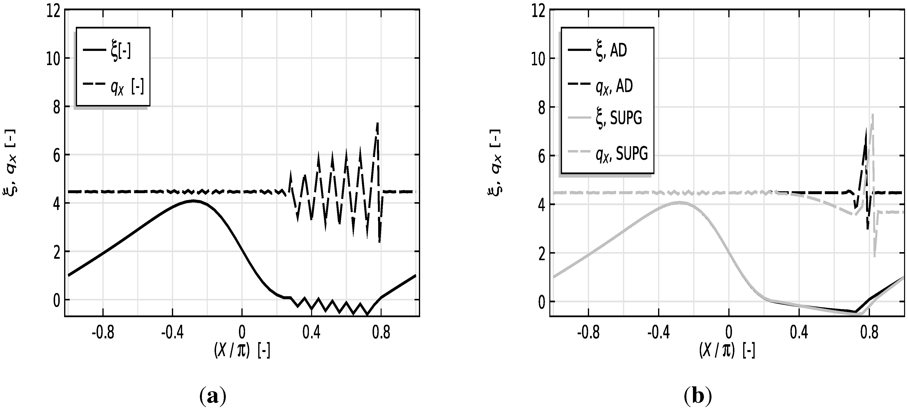It is difficult to solve Equation (9) using the standard Galerkin finite element approach because in the cavitated region $(\xi <0)$, the equation is purely convection dominated and, thus, will exhibit oscillations when solved using a standard Galerkin FEM. This can be observed in Figure 2a, where the dependent variable ξ and the dimensionless flow $\left(q_X\right)$ have been plotted against the dimensionless length. Plotting ξ provides direct insight into both the pressure and mass fraction distribution.

In the literature [17,18,19], one may find many approaches to numerically stabilize the FEM solution of the convection-dominated part in convection-diffusion equations. Some of these methods are the streamline upwind Petrov-Galerkin method (SUPG), the SU method and the artificial diffusion method (AD). The SUPG method adds an additional term to the test function to suppress the unwanted oscillations, whereas the SU method only adds the additional term to the convection-dominated part of the equation [19]. In the AD method, the diffusion part, of the convection-diffusion equation, is slightly modified with an additional artificial diffusion term in the convection-dominated part of the film.

Other techniques in the literature that deal with the convection-dominated aspect include semi-Lagrangian (or characteristic) methods [20,21]. The semi-Lagrangian technique has the advantage that it does not require the tuning parameters associated with the AD-method. However, this method requires substantial numerical effort and is not easily implemented in any general purpose software package, as it requires fundamental rewriting of the finite element code. Advanced general purpose FEM software is commonly used in the industry, as the lubrication problems usually encountered involve a multidisciplinary field, including thermal, structural, thermo-elastic and hydrodynamic simulations.

Hence, the chosen stabilization technique here is the artificial diffusion method (AD), as it can easily be implemented and only requires a slight modification to the coefficients in the general form PDE. In this method, the diffusion part in the convection-diffusion equation is slightly modified with an additional artificial diffusion term $k_{\text{AD}}$ in the convection-dominated part of the film:

$$\frac{\partial }{\partial X}\left(-\left(\frac{H^{3}f(\xi \ge 0)}{\tilde{\eta }}+(\xi <0)k_{\mathrm{AD}}\right)\frac{\partial \xi }{\partial X}+6Hf\right)=0$$

(10)

Note that the solution obtained using this method should be examined carefully as a slightly modified PDE is solved instead of the original one. Moreover, $k_{\text{AD}}$ should not be so large as to introduce excessive damping, but should be minimal just to suppress the generated oscillations. Hence, an optimum value for $k_{\text{AD}}$ needs to be chosen. The artificial diffusion coefficient $k_{\text{AD}}$ is chosen as follows:

$$k_{\mathrm{AD}}={\alpha }_0{\alpha }_{\mathrm{AD}}{h}_{e}u$$

(11)

where $h_e$ is a typical element size in the streamline direction and ${\alpha }_0$ is a constant that depends on the order of the elements that are used with ${\alpha }_0=0.5$ for linear elements and ${\alpha }_0=0.25$ for quadratic elements [22]. In the present analysis, linear elements are used. u and k are respectively equivalent to the velocity and diffusion coefficient in a typical convection-diffusion equation and can be calculated as follows:

$$\begin{array}{}\mathrm{(12a)}& \hfill u& =6H(\xi <0)c_f\hfill \mathrm{(12b)}& \hfill k& =H^{3}f(\xi \ge 0)\hfill \end{array}$$

${\alpha }_{\text{AD}}$ is an upwind function and can (after making an asymptotic approximation [22]) be computed as follows:

$${\alpha }_{\mathrm{AD}}=\min \left(P{e}_{\mathrm{AD}}/3,1\right)$$

(13)

where $P{e}_{\text{AD}}$ is the cell Peclet number $(P{e}_{\text{AD}}=\frac{u{h}_e}{2k})$. Due to the Boolean expressions, $P{e}_{\text{AD}}$ becomes zero in the full film region and infinite in the cavitated region. Consequently, the upwind function ${\alpha }_{\text{AD}}$ reduces to one in the cavitated region and zero in the full film region. Substituting Equation (11) into Equation (10) results in the following Reynolds equation:

$$\frac{\partial }{\partial X}\left(-\left(\frac{H^3\left(\xi \ge 0\right)}{\tilde{\eta }}+3h_{e}H(\xi <0)c_f\right)\frac{\partial \xi }{\partial X}+6Hf\right)=0$$

(14)

This equation is strongly non-linear due to the included Boolean expressions. After discretization using finite elements, the system of non-linear equations is solved using a simple fixed-point iteration where the Boolean expressions are evaluated by means of the solution of the previous iteration, which then results in a linear system of equations.

The dependent variable ξ and flow $q_X$ are plotted in Figure 2b after solving Equation (14). The results are compared with another streamline stabilization technique (SUPG) in Figure 2b from which it can be concluded that the results obtained using AD and SUPG are in close agreement.

Figure 2. Dependent variable ξ and flow $q_X$ against the dimensionless length of the fluid domain, without (left) and with numerical stabilization. $\tilde{\eta }$ = 1, $c_f$ = 1 and ε = 0.4. (a) FEM solution of the 1D Reynolds equation without stabilization, showing oscillations in the convection-dominated cavitated region; (b) comparison of the artificial diffusion (AD) and streamline upwind Petrov-Galerkin (SUPG) stabilization methods, showing similar results of the pressure and mass fraction. The discontinuity of the flow is not yet minimized here.

Figure 2. Dependent variable ξ and flow $q_X$ against the dimensionless length of the fluid domain, without (left) and with numerical stabilization. $\tilde{\eta }$ = 1, $c_f$ = 1 and ε = 0.4. (a) FEM solution of the 1D Reynolds equation without stabilization, showing oscillations in the convection-dominated cavitated region; (b) comparison of the artificial diffusion (AD) and streamline upwind Petrov-Galerkin (SUPG) stabilization methods, showing similar results of the pressure and mass fraction. The discontinuity of the flow is not yet minimized here.

Some discontinuity of flow at the reformation boundary remains, however, which should be continuous from the physical perspective. Minimization of this discontinuity can be obtained by choosing an optimum value for the transformation constant $c_f$. An attempt to resolve this challenge is by equating the flows at this boundary and working out using numerical differences; or:

$$\begin{array}{}\mathrm{(15a)}& \hfill q_{X_{\mathrm{cav}.}}& =q_{X_{\mathrm{full}.}}\iff \hfill \mathrm{(15b)}& \hfill {\left(6Hf\left(\xi \right)\right)}_{\mathrm{cav}.}& ={\left(\frac{-H^3}{\tilde{\eta }}\frac{\partial P}{\partial X}+6H\right)}_{\mathrm{full}.}\hfill \end{array}$$

where $q_{X,\text{cav}}$ and $q_{X,\text{full}}$ stand for the flow in the cavitated and full film region, respectively. Substituting the proposed transformation (Equation (8a) and (8b)) into Equation (15b) and working out in terms of numerical differences gives:

$$\begin{array}{}\mathrm{(16a)}& \hfill 6H_r\left(1+c_f{\xi }_r\right)& =\frac{-H_r^3}{\tilde{\eta }}\frac{{\xi }_{r+1}-{\xi }_r}{h_e}+6H_r\hfill \mathrm{(16b)}& \hfill c_f& =\frac{H_r^2\left(1-\frac{{\xi }_{r+1}}{{\xi }_r}\right)}{6\tilde{\eta }{h}_e}\hfill \end{array}$$

where $H_r$ and ${\xi }_r$ are the film thickness and solution at this interface point. The partial derivative is approximated using the numerical difference between the values of point r and downstream neighboring point $r+1$. In the cavitated region, the pressure is less than zero $({\xi }_r<0)$, whereas in the full film region, the pressure is equal to or larger than zero $({\xi }_{r+1}\ge 0)$. According to this, a critical transformation constant $\left(c_f^{*}\right)$ may be introduced, which complies with the following expression:

$$c_f\ge c_f^{*}=\frac{H_r^2}{6\tilde{\eta }{h}_e}$$

(17)

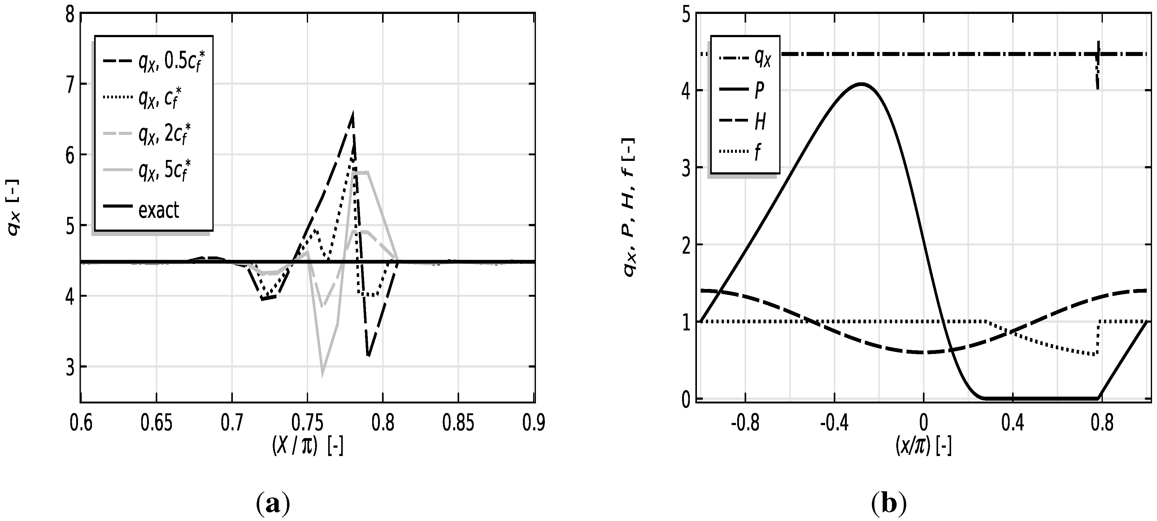
For values $c_f$ close to $c_f^{*}$, the discontinuity at the reformation boundary was minimal, and faster convergence was achieved; see Figure 3a. As can be observed, $c_f^{*}$ depends on the local height at the reformation interface, which is initially unknown. However, after performing some numerical experiments, it was observed that in most cases, $H_r$ is found to be very close to the maximum film height of the oil film. Hence, the maximum film height was used in the calculation of $c_f$.

With the dependence of $c_f^{*}$ on $H_r$, Equation (14) can now be simplified by suggesting $c_f=\frac{H^2}{3\tilde{\eta }{h}_e}$.

$$\frac{\partial }{\partial X}\left(-\frac{H^3}{12\tilde{\eta }}\frac{\partial \xi }{\partial X}+\frac{Hf}{2}\right)=0$$

(18)

Note the absence of any Boolean functions in the pressure term. This optimized transformation results in fast convergence, as it is slightly less non-linear and, thus, more stable. In Figure 3b, the mass fraction, film thickness, flow and pressure are plotted after solving Equation (18). It is clear that the flow discontinuity is minimal now. Note that due to this chosen value of $c_f=\frac{H^2}{3\tilde{\eta }{h}_e}$, which is dependent on the local element size $h_e$, the flow discontinuity is effectively minimized by locally refining the mesh size near the reformation boundary.

Figure 3. Distribution of mass fraction, film thickness, flow and pressure for $\tilde{\eta }$ = 1 and $\epsilon =0.4$. (a) Flow in the area near the reformation boundary using values close to the optimal transformation constant $c_f^{*}$. Note that the maximum film height was used for the calculation of $c_f^{*}$. (b) Solution of the 1D Reynolds equation (Equation (18)) using $c_f=\frac{H^2}{3\tilde{\eta }{h}_e}$, showing only minimum flow discontinuity.

Figure 3. Distribution of mass fraction, film thickness, flow and pressure for $\tilde{\eta }$ = 1 and $\epsilon =0.4$. (a) Flow in the area near the reformation boundary using values close to the optimal transformation constant $c_f^{*}$. Note that the maximum film height was used for the calculation of $c_f^{*}$. (b) Solution of the 1D Reynolds equation (Equation (18)) using $c_f=\frac{H^2}{3\tilde{\eta }{h}_e}$, showing only minimum flow discontinuity.

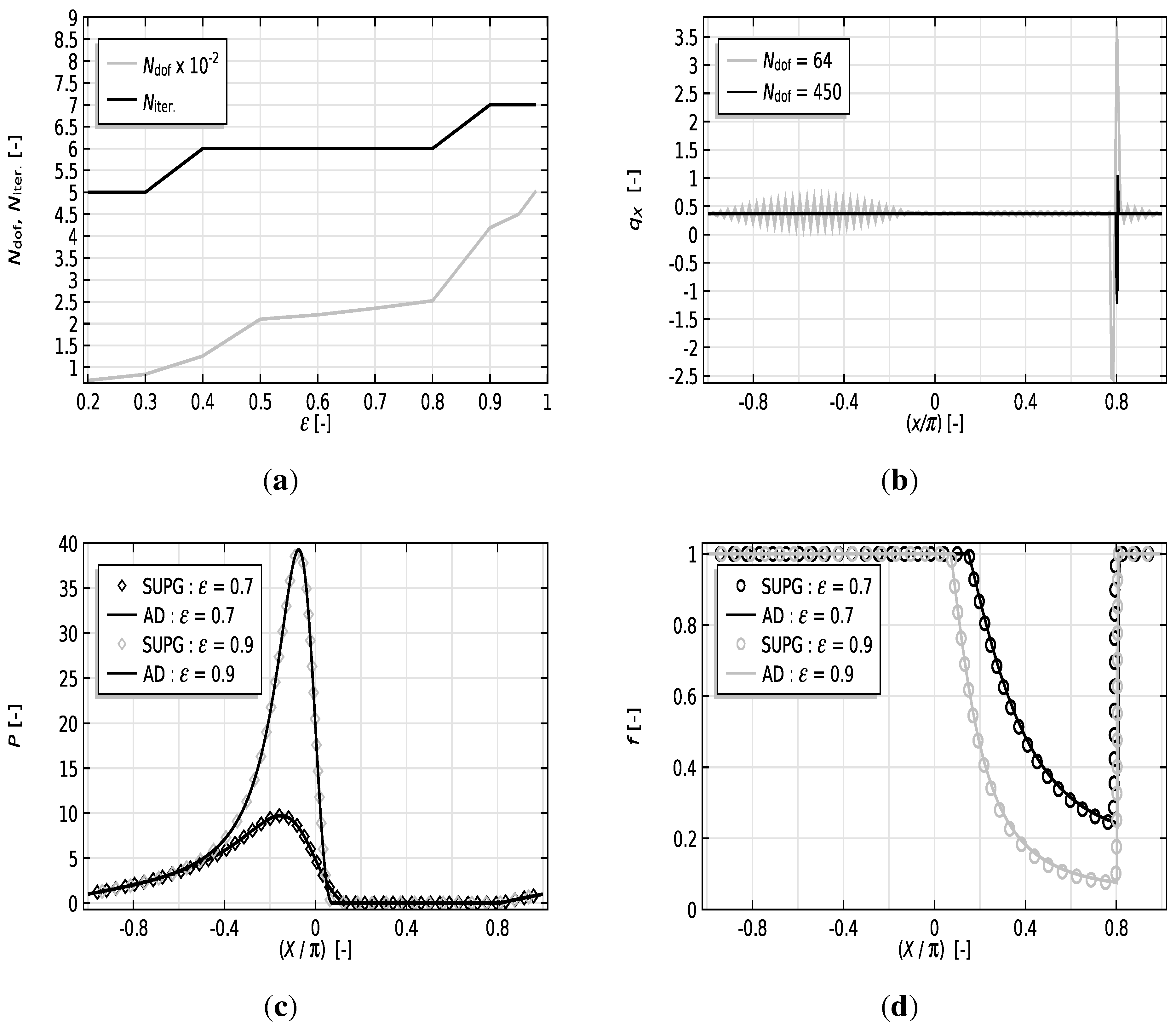
This 1D cavitation algorithm has been verified for the full range of shaft eccentricity values and for a large range of mesh densities, for low to high numbers of degrees of freedom $N_{\text{dof}}$. Figure 4a gives a representation of the required number of iterations $N_{\text{iter.}}$ and $N_{\text{dof}}$, in order to obtain relative errors of ${10}^{-4}-{10}^{-5}$, as a function of ε. As can be observed, the maximum number of iterations required is seven, which contributes as evidence for fast convergence. Typically, the computation time is within a few seconds on a quad core desktop computer.

It should be noted that if one only considers the pressure and/or the mass fraction profiles, it may seem that the solution is smooth enough. The streamline flow $q_X$, however, may exhibit oscillations due to the existence of steep pressure gradients, in particular at higher values for ε. Of course, this means that the mesh size has to be chosen smaller. This problem is clearly exposed in Figure 4b.

Figure 4c,d shows that the results obtained using our AD-stabilized cavitation algorithm are identical to "exact" results calculated by SUPG-stabilization, even for relatively high values of ε. This comparison shows the numerical robustness of the cavitation algorithm for high ε values.

Figure 4. Verification and/or representation of the numerical stability of the cavitation model for the full range of shaft eccentricities. $\tilde{\eta }$ = 1. (a) $N_{\text{dof}}$ and $N_{\text{iter.}}$ are associated with ε in order to obtain an optimum combination of accuracy and computational expense for the 1D model; (b) the influence of $N_{\text{dof}}$ on the streamline flow distribution for $\epsilon =0.95$. Note the oscillations in the solutions for a lower value of $N_{\text{dof}}$. (c) Comparison between pressure distributions obtained using the AD method with the SUPG method for relatively high eccentricity ratios. The results strictly follow each other. (d) Comparison between mass fraction distributions obtained using the AD method with the SUPG method. Even for high ε, minimal discontinuity is observed near the reformation boundary. Furthermore, excellent agreement exists between the results obtained using both methods.

Figure 4. Verification and/or representation of the numerical stability of the cavitation model for the full range of shaft eccentricities. $\tilde{\eta }$ = 1. (a) $N_{\text{dof}}$ and $N_{\text{iter.}}$ are associated with ε in order to obtain an optimum combination of accuracy and computational expense for the 1D model; (b) the influence of $N_{\text{dof}}$ on the streamline flow distribution for $\epsilon =0.95$. Note the oscillations in the solutions for a lower value of $N_{\text{dof}}$. (c) Comparison between pressure distributions obtained using the AD method with the SUPG method for relatively high eccentricity ratios. The results strictly follow each other. (d) Comparison between mass fraction distributions obtained using the AD method with the SUPG method. Even for high ε, minimal discontinuity is observed near the reformation boundary. Furthermore, excellent agreement exists between the results obtained using both methods.

To further validate our algorithm, the cavitation algorithm was used in several case studies for which there are reliable benchmark solutions in the literature. Giacopini et al. [23] developed a mass-conserving cavitation algorithm based on the concept of complementarity and successfully verified their model using several case studies with (semi)-analytical and numerical formulations. In the present paper, the proposed cavitation model will be adapted to three different case studies in order to test its numerical properties and finally verify the results with those of Giacopini et al. [23].

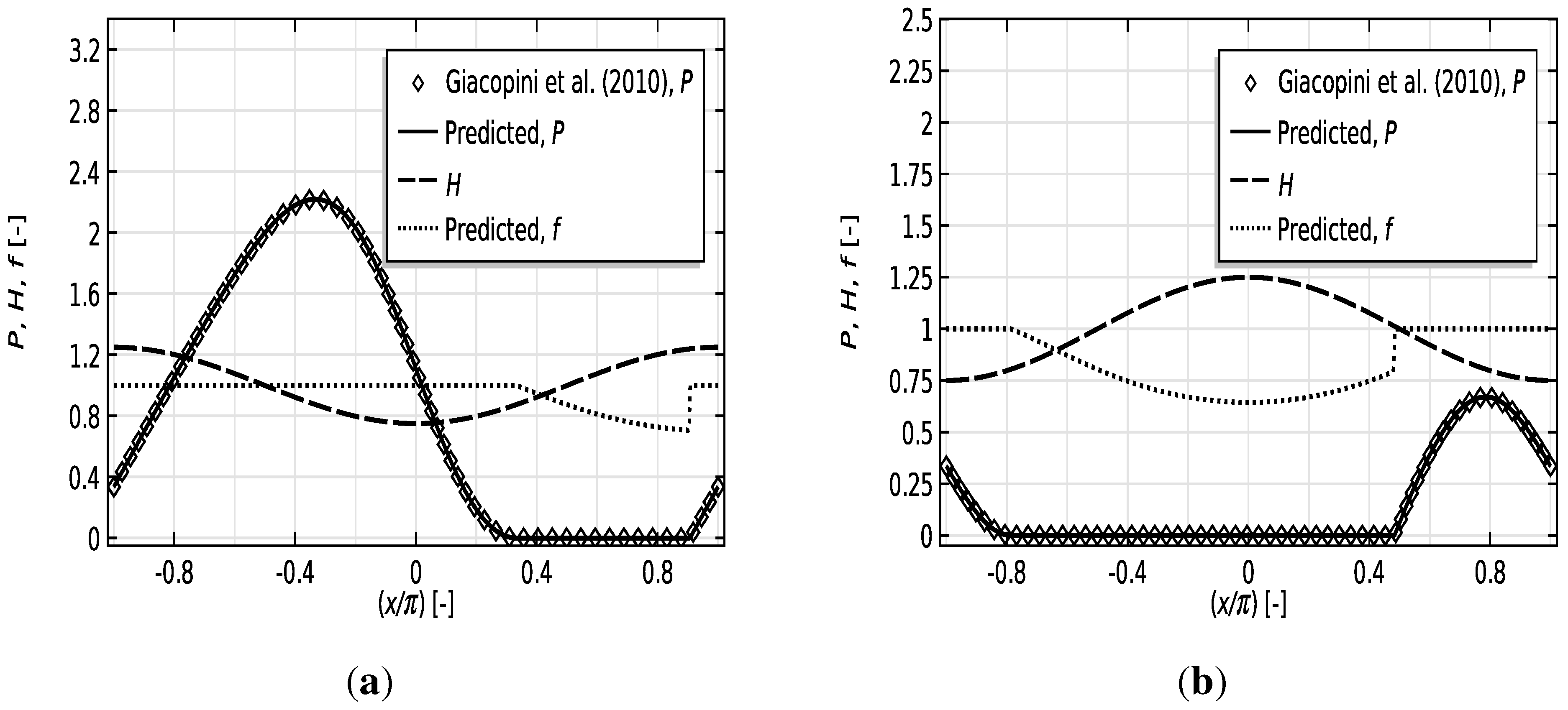
The first situation represents a simple journal bearing with an infinite width (see Figure 5a). The dimensions and relevant operating conditions are given in Figure 5. As can be observed, the film rupture and reformation boundary are accurately calculated. Excellent agreement is found between the predicted and reference pressure profiles.

The second situation is somewhat different, as the film thickness profile has a divergent-convergent shape (see Figure 5b). As can be extracted from Figure 5b, the film cavitates in the diverging region. Again, there is excellent accordance among both the predicted and reference results. Note that the diverging-converging shape of the film thickness can also be considered to be an idealization for situations involving surface texture.

Figure 5. Comparisons between predictions of the presented method with Giacopini et al. [23] for an infinite width sinusoidal bearing. Operating conditions for the present case are [23]: $h_0=0.02$ mm, $2\pi R=125$ mm, $\eta =0.015$ Pa·s, $U=4$ m/s and Boundary Condition 1 (BC1): $p=1$ MPa. (a) Comparison of the predicted pressure distributions with Giacopini et al. [23] for $\epsilon =0.25$. There is excellent agreement between the results. (b) Comparison of the predicted pressure distributions with Giacopini et al. [23] for $\epsilon =-0.25$. Again, excellent accordance between the results is observed.

Figure 5. Comparisons between predictions of the presented method with Giacopini et al. [23] for an infinite width sinusoidal bearing. Operating conditions for the present case are [23]: $h_0=0.02$ mm, $2\pi R=125$ mm, $\eta =0.015$ Pa·s, $U=4$ m/s and Boundary Condition 1 (BC1): $p=1$ MPa. (a) Comparison of the predicted pressure distributions with Giacopini et al. [23] for $\epsilon =0.25$. There is excellent agreement between the results. (b) Comparison of the predicted pressure distributions with Giacopini et al. [23] for $\epsilon =-0.25$. Again, excellent accordance between the results is observed.

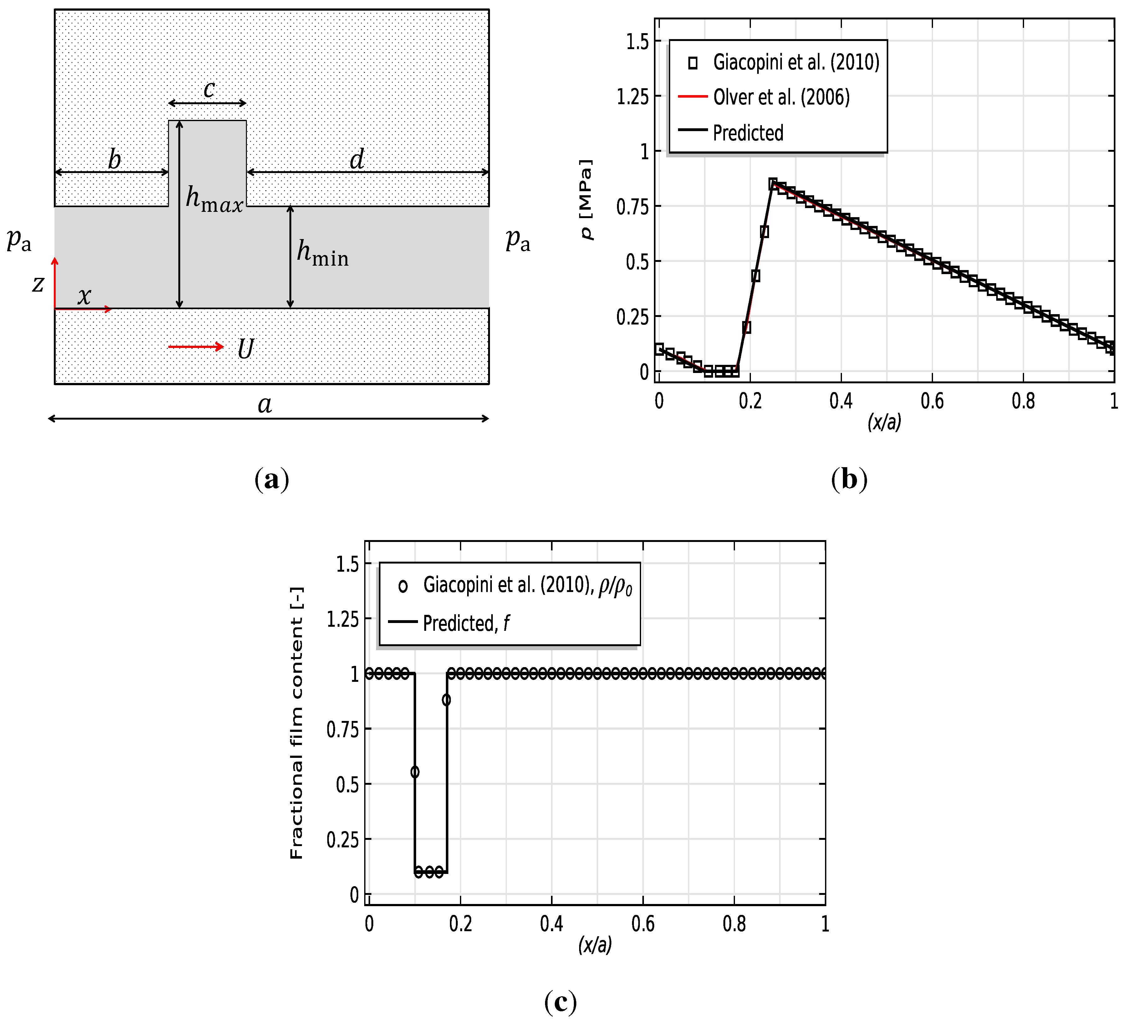
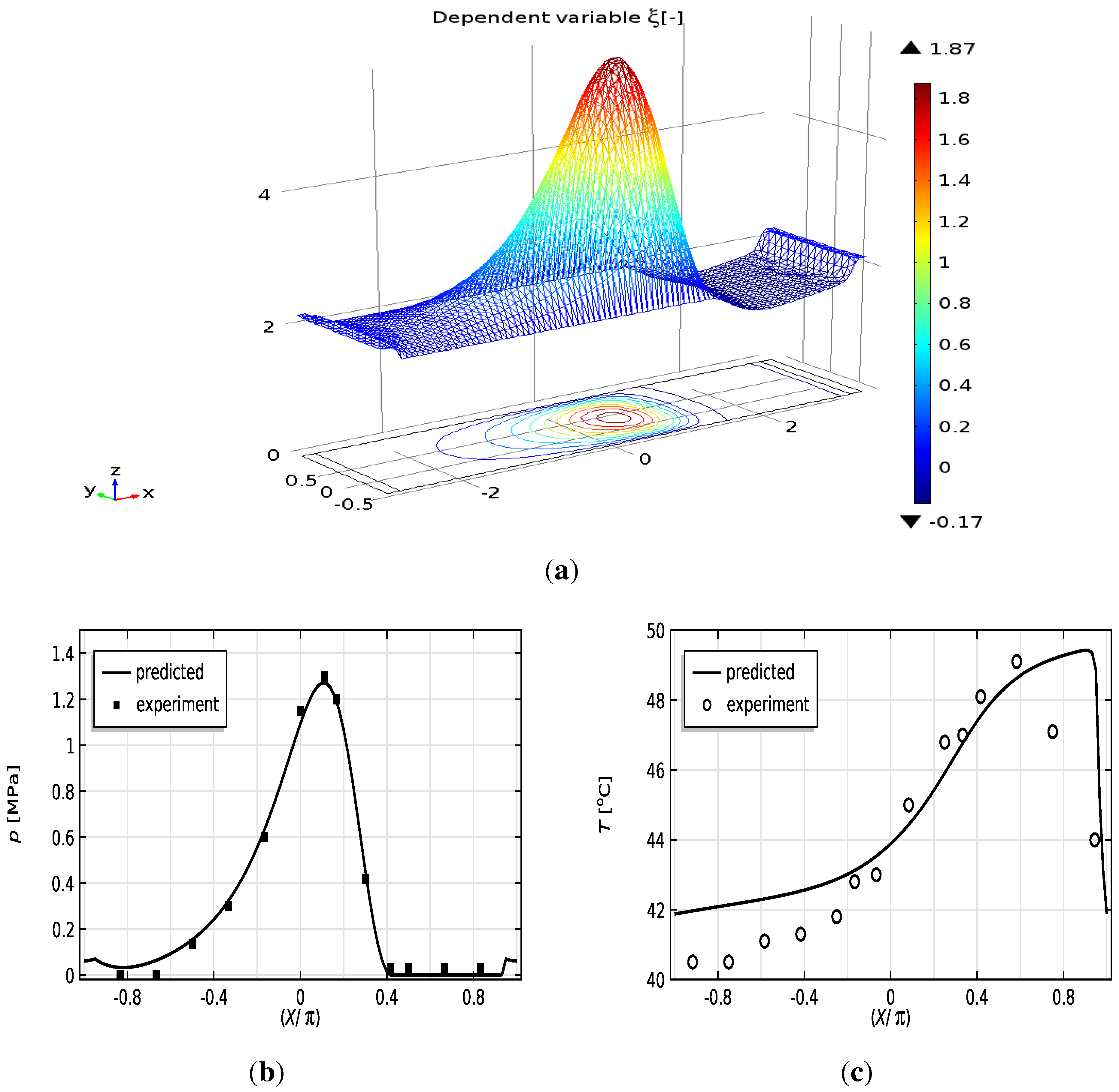
Hence, the last situation is that of a non-convergent/parallel bearing with a single microtexture pocket near the inlet (see Figure 6a). The reference dimensions and operating conditions are given in Figure 6. For this case, Olver et al. [24] derived an analytical solution, which pointed out the existence of a region in which the film cavitates. Comparisons of the predicted pressure profile with those of the reference authors are provided in Figure 6b in which the agreement is excellent. Figure 6c compares the predicted fractional film content distribution with the reference results in which fair accordance is obtained. Note that the fractional film content in the work of Giacopini et al. [23] is modeled using compressibility and is thus modeled as the non-dimensional density, which is why we have used a different notation for the fractional film content for the results of the reference authors. However, in the cavitated region, the pressure is constant, and thus, $\rho /{\rho }_0$ stands for the fractional film thickness.

Figure 6. Bearing configuration and comparisons between predictions of the presented method with past literature. Operating conditions for the present case are [23,24]: $b=2$ mm, $c=3$ mm, $d=15$ mm, $h_{\text{max}}=0.01$ mm, $h_{\text{min}}=0.001$ mm, $\eta =0.01$ Pa·s, $U=1$ m/s and $p_{\text{a}}=0.1$ MPa. (a) Schematic of a non-convergent/parallel bearing with a single microtexture pocket near the inlet. One surface is moving with velocity U, while the opposing surface is kept stationary. (b) Comparison of the predicted pressure distribution with Giacopini et al. [23] and the analytical solution of Olver et al. [24]. The results closely follow each other. (c) Comparison of the predicted fractional film content distribution with Giacopini et al. [23]. There is fair accordance between the results.

Figure 6. Bearing configuration and comparisons between predictions of the presented method with past literature. Operating conditions for the present case are [23,24]: $b=2$ mm, $c=3$ mm, $d=15$ mm, $h_{\text{max}}=0.01$ mm, $h_{\text{min}}=0.001$ mm, $\eta =0.01$ Pa·s, $U=1$ m/s and $p_{\text{a}}=0.1$ MPa. (a) Schematic of a non-convergent/parallel bearing with a single microtexture pocket near the inlet. One surface is moving with velocity U, while the opposing surface is kept stationary. (b) Comparison of the predicted pressure distribution with Giacopini et al. [23] and the analytical solution of Olver et al. [24]. The results closely follow each other. (c) Comparison of the predicted fractional film content distribution with Giacopini et al. [23]. There is fair accordance between the results.

2.2. 2D Stationary Situation: Crosswind Numerical Stabilization

In the previous section, the 1D cavitation algorithm was shown to be stable and robust and, moreover, produces results identical to the results found in the literature. Therefore, the algorithm will now be extended to a 2D cavitation algorithm. The extension of the stabilized 1D Reynolds equation (Equation (18)) to a 2D finite length journal bearing reads:

$$\frac{\partial }{\partial X}\left(\frac{-H^3}{12\tilde{\eta }}\frac{\partial \xi }{\partial X}+\frac{Hf}{2}\right)+\frac{\partial }{\partial Y}\left(\frac{-H^3\left(\xi \ge 0\right)}{12\tilde{\eta }}\frac{\partial \xi }{\partial Y}\right)=0$$

(19)

For this case, the supply is over the full bearing length (BC1: $P=1$), and the pressure on the edges of the bearing is set equal to zero (BC2: $P=0$). Furthermore, a relatively coarse grid is used to show the numerical stability of the stabilization techniques used.

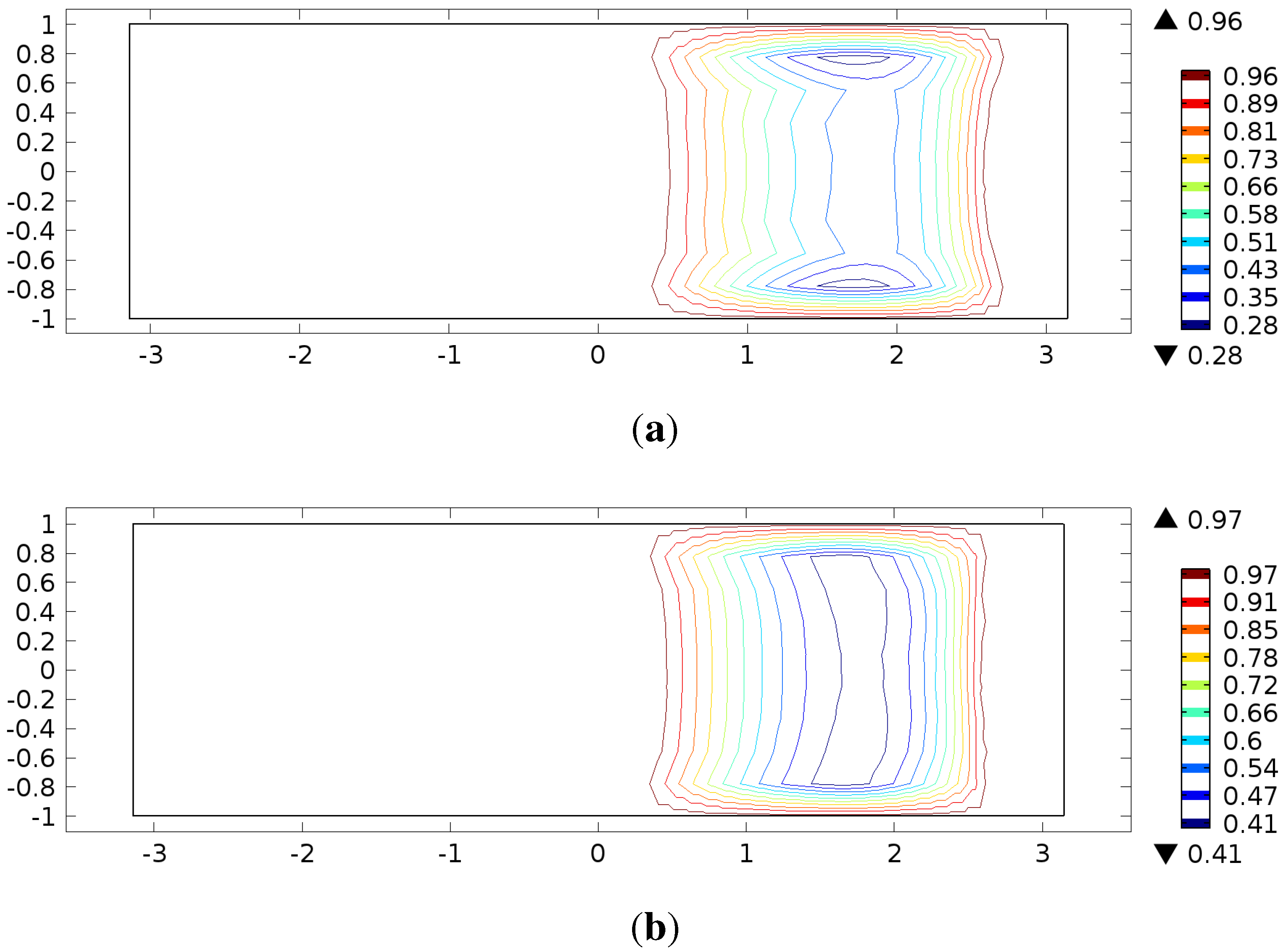
When Equation (19) is solved without further stabilization, the distribution of the mass fraction is not smooth, and spikes occur at the edges of the bearing, as can be seen in Figure 7a. This means that only applying streamline stabilization is not sufficient. Numerical stabilization is required in the crosswind direction (Y-direction), as well as in order to smooth the solution of the flow in the cavitated region. In Hughes et al. [19], Codina [22] and Tezduyar and Park [25], for instance, methods have been studied to choose the crosswind artificial diffusion coefficient. In this study, the diffusion term in the Y-component of the Reynolds equation is modified by adding an artificial diffusion term $k_{\text{AD},Y}$:

$$\frac{\partial }{\partial X}\left(\frac{-H^3}{12\tilde{\eta }}\frac{\partial \xi }{\partial X}+\frac{Hf}{2}\right)+\frac{\partial }{\partial Y}\left(\frac{-H^3}{12\tilde{\eta }}\left(\left(\xi \ge 0\right)+(\xi <0)k_{\mathrm{AD},Y}\right)\frac{\partial \xi }{\partial Y}\right)=0$$

(20)

In this study, the crosswind diffusion coefficient is chosen similar to $k_{\text{AD}}$, but scaled relative to the angle between the flow solution gradient and flow direction. The crosswind artificial diffusion coefficient $k_{\text{AD},Y}$ is chosen as follows:

$$\begin{array}{}\mathrm{(21a)}& \hfill k_{\mathrm{AD},Y}& =k_{\mathrm{AD},Y}^{*}{k}_{\mathrm{AD}}\hfill \mathrm{(21b)}& \hfill k_{\mathrm{AD},Y}^{*}& =\left(\frac{\left|\frac{\partial \xi }{\partial X}\right|\left|\frac{\partial \xi }{\partial Y}\right|}{{\left(\frac{\partial \xi }{\partial X}\right)}^2+{\left(\frac{\partial \xi }{\partial Y}\right)}^2+\delta }\right)\hfill \end{array}$$

where δ is a very small number (order of magnitude 1e-10) to prevent numerical problems in areas where the gradients $\frac{\partial \xi }{\partial X}$ and $\frac{\partial \xi }{\partial Y}$ are zero. Substituting this value for $k_{\text{AD},Y}$ in Equation (20) results in the stationary cavitated-modified Reynolds equation for a 2D lubricating film:

$$\frac{\partial }{\partial X}\left(\frac{-H^3}{12\tilde{\eta }}\frac{\partial \xi }{\partial X}+\frac{Hf\left(\xi \right)}{2}\right)+\frac{\partial }{\partial Y}\left(\frac{-H^3}{12\tilde{\eta }}\left(\left(\xi \ge 0\right)+(\xi <0)k_{\mathrm{AD},Y}^{*}\right)\frac{\partial \xi }{\partial Y}\right)=0$$

(22)

A convergence analysis was performed from which it was concluded that an optimum combination of accuracy and the number of elements is obtained at $N_{\text{dof}}=$ 4100 (approximately 8050 linear elements). Relative errors of approximately ${10}^{-4}-{10}^{-5}$ are usually found within 10–15 iterations. Typically, the computation time is within 10 s on a quad core desktop computer.

Figure 7. Mass fraction contours with and without crosswind numerical stabilization for $\tilde{\eta }$ = 1 and ε = 0.6. (a) Only streamline stabilization, i.e., $k_{\mathrm{AD},Y}=0$ showing spikes in the Y-direction near the edges; (b) non-linear crosswind stabilization suppresses the spikes.

Figure 7. Mass fraction contours with and without crosswind numerical stabilization for $\tilde{\eta }$ = 1 and ε = 0.6. (a) Only streamline stabilization, i.e., $k_{\mathrm{AD},Y}=0$ showing spikes in the Y-direction near the edges; (b) non-linear crosswind stabilization suppresses the spikes.

Solving Equation (22) using a typical PDE routine gives a reasonable solution, as the overshoot for the mass fraction distribution is almost suppressed and the sharp transition at the edge of the bearing is retained; see Figure 7b. Several other non-linear crosswind numerical stabilization techniques have also been tested, but the one represented by Equation (21) has been shown to be most stable and the fastest to converge.

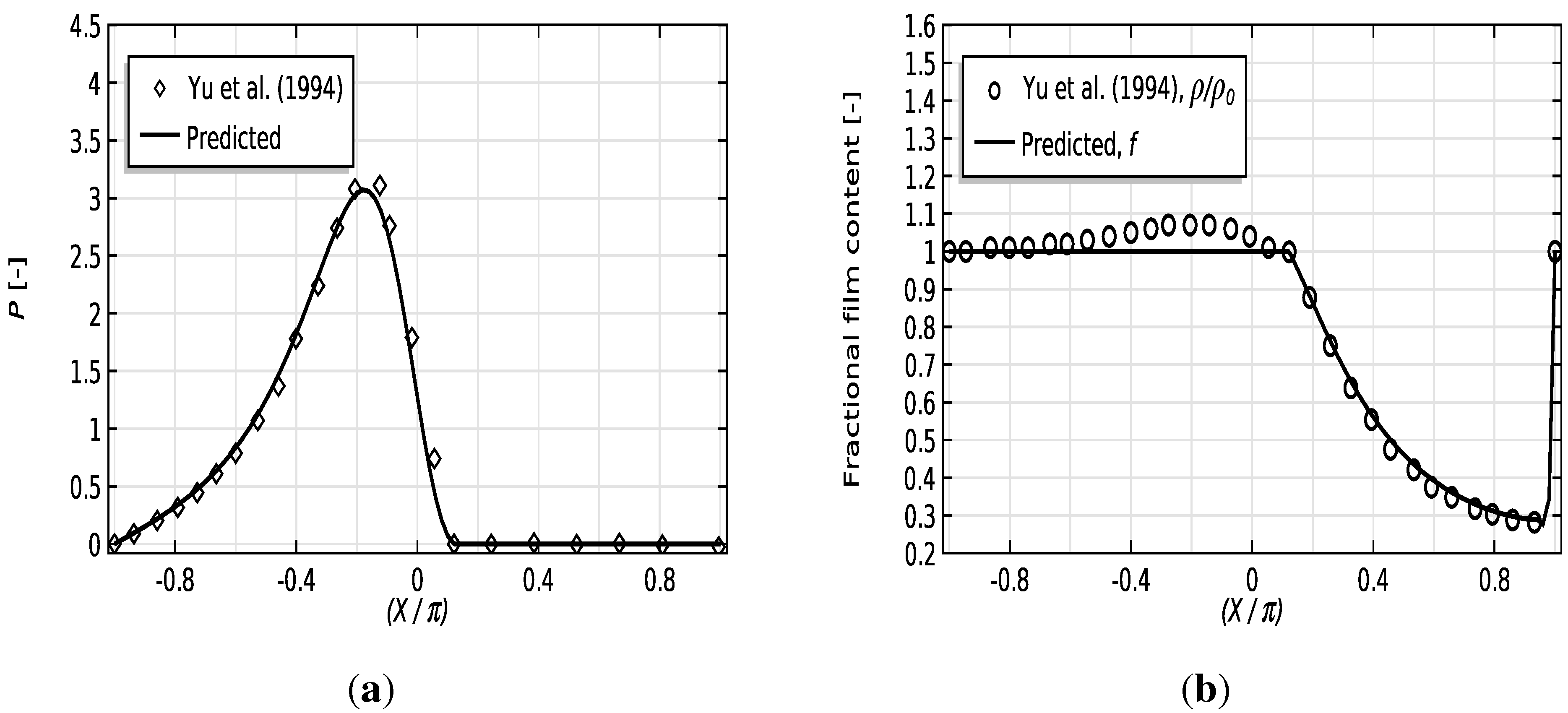
The artificial diffusion term for the crosswind stabilization slightly changes the original Reynolds PDE. In order to see if the results after this modification are still accurate, our cavitation algorithm was compared with those from Yu et al. [26] for a fully submerged bearing. Yu transformed Elrod’s universal differential equation into a boundary integral equation by means of boundary element theory and compared their results with those obtained using a finite difference approach in which they found excellent accordance. Typical Dirichlet conditions ($P=0$) are imposed on all edges of the computational domain. The pressure and mass fraction distributions are compared in Figure 8a,b, respectively, from which it is clear that the results closely follow each other. As mentioned earlier, the fractional film content in the full film region of the reference results is modeled using compressibility, which is the reason why the non-dimensional density slightly increases in that region.

Based on this comparison, it can safely be stated that the artificial diffusion terms have little influence on the overall solution accuracy, and thus, the AD-method may be used.

Figure 8. Steady-state validation of the proposed 2D cavitation model with Yu et al. [26] for $\tilde{\eta }$ = 1 and ε = 0.6. The graphs are plotted at an axial location of Y = 0.2 for the sake of comparison. (a) Comparison of pressure distributions; (b) comparison of mass fraction distributions.

Figure 8. Steady-state validation of the proposed 2D cavitation model with Yu et al. [26] for $\tilde{\eta }$ = 1 and ε = 0.6. The graphs are plotted at an axial location of Y = 0.2 for the sake of comparison. (a) Comparison of pressure distributions; (b) comparison of mass fraction distributions.

2.3. 2D Transient Situation: Equations of Motion

For a time-dependent problem, the squeeze term $\left(\frac{\partial \left(fH\right)}{\partial \tilde{t}}\right)$ needs to be added to Equation (22). The stabilized 2D cavitated-Reynolds equation then becomes:

$$\frac{\partial q_X}{\partial X}+\frac{\partial q_Y}{\partial Y}+\left(f+2c_f\left(\xi <0\right)\xi \right)\frac{\partial H}{\partial \tilde{t}}+H{c}_f\left(\xi <0\right)\frac{\partial \xi }{\partial \tilde{t}}=0$$

(23)

with the dimensionless circumferential and axial flows, respectively:

$$\begin{array}{}\mathrm{(24a)}& \hfill q_X& =\frac{-H^3}{12\tilde{\eta }}\frac{\partial \xi }{\partial X}+\frac{Hf}{2}\hfill \mathrm{(24b)}& \hfill q_Y& =\frac{-H^3}{12\tilde{\eta }}\left(\left(\xi \ge 0\right)+(\xi <0)k_{\mathrm{AD},Y}^{*}\right)\frac{\partial \xi }{\partial Y}\hfill \end{array}$$

An inverse bearing model is used here: it is assumed that the applied load $W^{\mathrm{a}}$ and load angle $X_W$ are known, and the corresponding eccentricity ε and attitude angle $X_{\epsilon }$ have to be calculated. Note that the load vectors are dependent on the pressure and therefore on the eccentricity and attitude angle.

In case an external force $\left(W^{\mathrm{a}}\right)$ is acting on the shaft, this force and the load carrying force of the lubricating film combine, and the resulting equations of motion become:

$$\left[\begin{array}{c}{W}_{\overline{x}}\\ W_{\overline{y}}\end{array}\right]+\left[\begin{array}{c}{W}_{\overline{x}}^{\mathrm{a}}\\ W_{\overline{y}}^{\mathrm{a}}\end{array}\right]=M\left[\begin{array}{c}{\ddot{\epsilon }}_{\overline{x}}\\ {\ddot{\epsilon }}_{\overline{y}}\end{array}\right]$$

(25)

where M represents the reduced mass of the system. M, $W_{\overline{x}},W_{\overline{y}}$ and $X_W$ are given by:

$$\begin{array}{}\mathrm{(26a)}& \hfill M& =\frac{m{h}_0^3{\omega }^2}{{\eta }_{0}U{R}^3}\hfill \mathrm{(26b)}& \hfill W_{\overline{x}}& ={\int }_{\Omega }-Pcos\left(X\right)d\Omega \hfill \mathrm{(26c)}& \hfill W_{\overline{y}}& ={\int }_{\Omega }-Psin\left(X\right)d\Omega \hfill \mathrm{(26d)}& \hfill X_W& =\arctan \left(\frac{W_{\overline{y}}}{W_{\overline{x}}}\right)\hfill \end{array}$$

Equations (25) and (26) are simultaneously solved using a modified Newton-Raphson iteration scheme from which the correct load angle and eccentricity are obtained.

3. Expansion to a Thermo-Hydrodynamic Model

In the previous section, a novel and fast mass-conserving Reynolds cavitation algorithm was developed, from which the mass fraction and the pressure distribution throughout the fluid film domain can be calculated. In general, modeling a plain journal bearing using the assumption of an isoviscous fluid leads to unrealistic results [4]. Hence, in this section, a simple and efficient thermal model is developed from which the viscosity distribution can be obtained. Furthermore, in the previous section, it was assumed that the supply groove was infinitely small in the circumferential direction. In this section, the shape of the supply groove and its influence on the temperature and pressure distribution is taken into account.

In addition to the variables of Equation (4), the following dimensionless variables are introduced:

$$\begin{array}{cccccccc}\hfill \tilde{k}& =\frac{k}{U{C}_{p}R{\rho }_0}\hfill & \hfill \tilde{T}& =\frac{h_0^2{\rho }_0{C}_p}{R{\eta }_{0}U}(T-T_s)\hfill & \hfill \tilde{\varphi }& =\frac{\varphi h_0}{U^2{R}^2{\eta }_0}\hfill & \hfill \tilde{Q}& =\frac{Q}{RU{h}_0}\hfill \end{array}$$

(27)

3.1. Fluid Rheology

In this model, the viscosity is a function of temperature $\tilde{T}$ based on the following exponential expression:

$$\tilde{\eta }=e^{-\tilde{\beta }\tilde{T}}$$

(28)

where $\tilde{\beta }$ stands for the dimensionless temperature viscosity coefficient. The shear rate and pressure dependencies of viscosity are not taken into account in this analysis, but could straightforwardly be taken into account in the methods presented in this section.

3.2. Energy Equation and Oil Supply

The heat transport calculations are based on the assumption of adiabatic conditions, i.e., heat transport to and from the bearing housing and the shaft are neglected. This follows from the assumption that convective heat transport is dominant, i.e., the lubricant leaving the bearing carries away the major part of heat generated in the film. Furthermore, the use of an effective temperature across the film thickness is made. This reduces the 3D energy model to a simple and efficient 2D model. From these simplifications, the adiabatic energy equation reads [27]:

$$\left[\frac{\partial }{\partial X}\left(q_X\tilde{T}-\tilde{k}Hf\frac{\partial \tilde{T}}{\partial X}\right)+\frac{\partial }{\partial Y}\left(q_Y\tilde{T}-\tilde{k}H\left(\xi \ge 0\right)\frac{\partial \tilde{T}}{\partial Y}\right)+Hf\frac{\partial \tilde{T}}{\partial \tilde{t}}\right]=\tilde{\psi }-\sum q_{\mathrm{m}}\tilde{T}$$

(29)

where $q_X$ and $q_Y$ are the bulk flow velocities in the X and Y-directions, respectively, obtained from Equations (24a) and (24b). The viscous dissipation term $\tilde{\psi }$ and friction losses $\tilde{\varphi }$ can be calculated as follows:

$$\begin{array}{}\mathrm{(30a)}& \hfill \tilde{\psi }& =\frac{H^3}{12\tilde{\eta }}\left[{\left(\frac{\partial P}{\partial X}\right)}^2+{\left(\frac{\partial P}{\partial Y}\right)}^2\right]+\frac{\tilde{\eta }f}{H}\hfill \mathrm{(30b)}& \hfill \tilde{\varphi }& ={\int }_{\Omega }\tilde{\psi }d\Omega \hfill \end{array}$$

where Ω stands for the bearing surface area. The second term on the RHS of Equation (29) denotes the inflow (heat flux) of oil from the supply groove(s) to the bearing. The calculation of this term follows later on in this section.

Equation (29) assumes that finger-type cavitation occurs, which means that the flow in the cavitation area consists of fluid streamers separated by pockets of gas. This means that in the cavitated region, heat conduction in the Y-direction can safely be ignored, as heat conduction through gas is far less than through oil. Hence, the Boolean expression in front of the heat conduction term is in the Y-direction. Heat generation in the cavitated regions is assumed to be solely generated due to shear losses in the streamers. Furthermore, the heat capacity k and heat conduction coefficient $C_p$ are assumed to be constant throughout the calculations, as their temperature and pressure dependency is much less compared to that of the viscosity.

Similar to the Reynolds equation, the thermal Equation (29) is strongly convection dominated and, hence, also requires numerical stabilization. To this end, we have implemented the SUPG method in order to stabilize the solution of Equation (29) in the cavitated region.

The temperature distribution in the supply grooves is calculated based on perfect mixing conditions (see, for instance, van Ostayen and van Beek [27]). The oil inflow from the supply grooves to the fluid film is calculated, taking into account the shape of the groove, by:

$$q_m=({\tilde{Q}}_m>0){\tilde{Q}}_m\frac{H_f}{{\int }_{{\Omega }_m}{H}_{f}d\Omega }$$

(31)

where ${\Omega }_{\mathrm{m}}$ stands for the surface area of the groove. In some cases, the hydrodynamically-generated pressure in the supply groove is larger than the supply pressure. In those situations, hot oil is forced back into the system $({\tilde{Q}}_m<0)$, and the Boolean function in Equation (31) is equal to zero, as no heat transport takes place. Weak Dirichlet pressure boundary conditions $(P=P_s)$ are imposed on the edges of the supply grooves. The volumetric flow in the groove can then be obtained by integrating the Lagrange-multiplier associated with the pressure, over the edges of the supply groove:

$${\tilde{Q}}_m={\int }_{{\Pi }_m}{\xi }_{\mathrm{lm}}ds$$

(32)

where ${\xi }_{\mathrm{lm}}$ represents the Lagrange-multiplier associated with the pressure P. The assumption has been made that the oil inflow from the supply grooves to the fluid film is distributed across the grooves relative to the local groove depth according to the following relation [27]:

$$H_f=H_{f,\max }\left(1-{\left(\frac{2(x-x_m)}{d_m}\right)}^2\right)\left(1-{\left(\frac{2y}{d_m}\right)}^2\right)$$

(33)

3.3. Boundary Conditions

At $X=-\pi$ and $X=\pi$ (BC1), periodicity is imposed to ensure flow continuity. On the edges of the supply groove, a typical Dirichlet boundary condition has been imposed with supply pressure $P_{\mathrm{s}}$. On the edges of the bearing (BC2), non-submerged boundary conditions are imposed, and the temperature gradient normal to the edges is assumed to be zero. The term “non-submerged” mathematically implies that in the full film areas, the pressure on the edges is set to zero $\left(\xi =0\right)$, as there is outflow of lubricant, whereas in the cavitated/inflow regions, zero flow is enforced (no boundary condition is set, 0 = 0). The non-submerged boundary condition can thus realistically be simulated using the following constraint:

$$\left(\xi \ge 0\right)\left(n_Y{q}_Y>0\right)\xi =0$$

(34)

where $n_Y$ is the normal vector of the edges.

4. Results

The developed model in the previous sections is solved using a general purpose finite element analysis software [12]. Notice the strong non-linear coupling between Equations (2), (6) and (26), where W and $X_W$ are a function of P and, therefore, a function of ε and $X_{\epsilon }$. Moreover, the variable viscosity $\left(\tilde{\eta }\right)$ couples the Reynolds equation with the energy equation.

Summarizing, the set of equations and constraints (load balances, the Reynolds and energy equation with its respective boundary conditions) is solved using this finite element formulation, where the resulting system of non-linear equations is solved using a monolithic approach, where all of the dependent variables $\left(\xi ,\tilde{T},\epsilon ,X_{\epsilon }\right)$ are collected in one vector of unknowns and simultaneously solved using a modified Newton-Raphson iteration scheme coupled with a time stepping algorithm. For a detailed description of the used time stepping algorithm and integration scheme, see [12].

4.1. Validation of the 2D THD Steady State Model

Ferron et al. [14] performed experiments on a single axial grooved bearing and obtained satisfactory accordance between simulations and measurements. Their measurements are regularly used as a benchmark for verification of THD models (for example [28,29,30]). In order to validate the proposed model, the bearing geometry and operating conditions used by Ferron et al. [14] are used for a numerical study (see Table 1). In the present work, the assumption of adiabatic bounding surfaces has been made after consideration of the operating conditions under which the experiments were performed.

Table 1. Geometric details of the plain journal bearing and properties of the lubricant for the reference calculations [14].

Parameter	Symbol	Value
Shaft diameter	d	100e-3 (m)
Axial length bearing	L	80e-3 (m)
Clearance	C	145e-6 (m)
Groove depth (assumed)	$H_{f,\max }$	2e-3 (m)
Density	ρ	860$(\mathrm{kg}/{\mathrm{m}}^3)$
(Inlet) viscosity	${\eta }_0$	0.0277 (Pa·s)
Heat capacity	$C_p$	2000 (J/kg·K)
Heat conduction coefficient	k	0.13 (W/(m·K))
Temperature-viscosity index	β	3.3e-2 (1/K)
Supply pressure	$p_{\mathrm{s}}$	0.7e5 (Pa)
Supply temperature	$T_{\mathrm{s}}$	40 (°C)
Groove angle	-	18°

Table 1. Geometric details of the plain journal bearing and properties of the lubricant for the reference calculations [14].

Parameter	Symbol	Value
Shaft diameter	d	100e-3 (m)
Axial length bearing	L	80e-3 (m)
Clearance	C	145e-6 (m)
Groove depth (assumed)	$H_{f,\max }$	2e-3 (m)
Density	ρ	860$(\mathrm{kg}/{\mathrm{m}}^3)$
(Inlet) viscosity	${\eta }_0$	0.0277 (Pa·s)
Heat capacity	$C_p$	2000 (J/kg·K)
Heat conduction coefficient	k	0.13 (W/(m·K))
Temperature-viscosity index	β	3.3e-2 (1/K)
Supply pressure	$p_{\mathrm{s}}$	0.7e5 (Pa)
Supply temperature	$T_{\mathrm{s}}$	40 (°C)
Groove angle	-	18°

A convergence analysis was performed for the reference operating conditions, from which it was concluded that an optimum combination of accuracy and the number of elements is obtained at $N_{\text{dof}}=$ 4100 (approximately 8050 linear elements), and hence, this mesh distribution is used further throughout the analysis. Relative errors of approximately ${10}^{-4}-{10}^{-5}$ are usually found within 15–25 iterations. Typically, the computation time is 20–25 s on a quad core desktop computer.

It is worth mentioning that in the paper of Ferron et al., the viscosity-pressure dependence was not taken into account, although this dependence may compensate in part for the viscosity reduction due to the temperature rise. The pressure viscosity coefficient for a typical mineral oil is in the range of ${10}^{-8}$ Pa${}^{-1}$. Thus, it is safe to ignore the viscosity-pressure dependence (as compared to the viscosity-temperature dependence) considering the order of magnitude of the pressures in Figure 9b.

In Figure 9a, the dependent variable ξ is plotted, in which the hydrodynamic pressure peak can clearly be observed. It can also be observed from Figure 9a that due to the imposed non-submerged boundary condition at the edges of the bearing (see Equation (34)), $\xi =0$ in the full film region, and no flow is enforced in the cavitated region.

The theoretical predictions are compared with the measurements of Ferron et al., in Figure 9b,c. Concerning the pressure profiles, excellent agreement is found. Note the jump in the pressure profile at both ends of the interval as a consequence of the imposed pressure constraint $P_{\mathrm{s}}$ at these ends (the supply groove has a finite width, which is defined by the groove angle (see Table 1)). There are, however, some discrepancies between the predicted and measured temperature profiles. As can be seen, the magnitude of the predicted maximum temperature is in accordance with the measured maximum temperature. The location of the maximum temperature is not accurately predicted, though. A probable explanation follows from the treatment of heat transport in the cavitated region. In this model, the assumption was made that the cavitated area consists of fluid streamers (finger-type cavitation). However, the actual behavior of fluid in the cavitated region may be different. Moreover, the oil inflow profile, which was assumed, Equation (33), might be inaccurate. It is known that the inflow of oil can have significant influence on the calculated temperature field and, hence, should be investigated in more detail.

Figure 9. Distributions of dependent variable ξ, pressure and temperature $w_{\overline{x}}^{\mathrm{a}}=4$ kN, ${\omega }_{\mathrm{s}}=2$ krpm. (a) Height expression and contour plot for the dependent variable ξ; (b) comparison of the theoretical and experimental [14] circumferential mid-plane $(Y=0)$ pressure profile; (c) comparison of the theoretical and experimental [14] circumferential mid-plane $(Y=0)$ temperature profile.

Figure 9. Distributions of dependent variable ξ, pressure and temperature $w_{\overline{x}}^{\mathrm{a}}=4$ kN, ${\omega }_{\mathrm{s}}=2$ krpm. (a) Height expression and contour plot for the dependent variable ξ; (b) comparison of the theoretical and experimental [14] circumferential mid-plane $(Y=0)$ pressure profile; (c) comparison of the theoretical and experimental [14] circumferential mid-plane $(Y=0)$ temperature profile.

In Figure 10a, the eccentricity ratio is plotted against the varied applied load: fair agreement is found between the measurements and the predictions. Satisfactory agreement is also found between the outflow of the lubricant as a function of the eccentricity ratio; see Figure 10b. A similar statement can be made about the maximum pressures as a function of the eccentricity ratio at different rotation speeds; see Figure 10c,d.

In Figure 10e,f, the maximum temperatures are plotted against the eccentricity ratio at different rotational speeds. As can be noticed, there are some discrepancies between the predictions and theory of the maximum temperatures. This might be due to the aforementioned assumptions of the cavitation type and the oil inlet profile. In addition, changes in clearance of the bearing due to thermal growth could also have caused discrepancies, which are not taken into account in our model. In general, it can be stated that satisfactory agreement between the measurements and the predictions is found.

Figure 10. Comparison of the modeling results with the measurements of Ferron et al. [14].

Figure 10. Comparison of the modeling results with the measurements of Ferron et al. [14].

4.2. Transient 2D THD Results

Although the reference results of Ferron [14] only contain steady-state results, a time transient analysis is performed here for the sake of completeness. The transient analysis is performed by means of applying a synchronous harmonic load on the journal, to demonstrate the performance of the journal bearing model under dynamic loading. The applied load in its respective $\overline{x}$- and $\overline{y}$-directions can be written as:

$$\left[\begin{array}{c}{W}_{\overline{x}}^{\mathrm{a}}\\ W_{\overline{y}}^{\mathrm{a}}\end{array}\right]=\left[\begin{array}{c}\left|W^{\mathrm{a}}\right|\cos \left(\tilde{t}\right)\\ \left|W^{\mathrm{a}}\right|\sin \left(\tilde{t}\right)\end{array}\right]$$

(35)

In Figure 11a, the shaft orbit resulting from the transient analysis is plotted. It is observed in Figure 11a,b that after, the initial transient effects, both pressure p and film thickness h, reach a limit cycle and continue to move in that cycle. Moreover, the solution for the maximum pressure and temperature in the limit cycle is in the vicinity of the steady-state solution (see Figure 11b and Figure 12). An interesting result that is provided is the behavior of the maximum temperature $T_{\max }$ with time, which is that it reaches equilibrium with the surroundings and, hence, approximates a steady value after a certain period of time. The typical computational time for the time-dependent calculation is 2–4 minutes per revolution on a typical quad core desktop computer.

Careful study of Figure 11a reveals that it is clear that the shape of the profile $(\epsilon ,X_{\epsilon },\tilde{t})$ is not a perfect circle, which means that the eccentricity $\left(\epsilon \right)$ has a maximum and a minimum (in this case, near an altitude angle $\left(X_{\epsilon }\right)$ of 180°). This was found to be due to the hydrostatic pressure of the oil inlet channel. As can be observed in Figure 11b, a peak pressure occurs every time the hydrodynamic peak pressure coincides with the start and end of the oil inlet channel, explaining the double pressure peaks each revolution. During this passage, also the supply flow decreases, which logically implies that less cold lubricant is introduced into the film (see Equation (31)) and, hence, results in a slight increase in temperature, which, after the passage of the oil inlet channel, decreases again to its former value (Figure 12).

Figure 11. Time-transient analysis for the reference bearing for $w^{\mathrm{a}}=4$ kN (dynamic loading) and ${\omega }_{\mathrm{s}}$ 2 krpm. (a) Shaft orbit; revolution of journal center locus with time. (b) Maximum pressure $\left(p_{\max }\right)$, minimum film thickness $\left(h_{\min }\right)$ and supply/outflow of lubricant $\left(Q_{\mathrm{supply}}\right)$.

Figure 11. Time-transient analysis for the reference bearing for $w^{\mathrm{a}}=4$ kN (dynamic loading) and ${\omega }_{\mathrm{s}}$ 2 krpm. (a) Shaft orbit; revolution of journal center locus with time. (b) Maximum pressure $\left(p_{\max }\right)$, minimum film thickness $\left(h_{\min }\right)$ and supply/outflow of lubricant $\left(Q_{\mathrm{supply}}\right)$.

Figure 12. Maximum temperature $\left(T_{\max }\right)$ evaluated at the mid-plane ($Y=0$) and mechanical losses due to shearing. Time-transient analysis. $w^{\mathrm{a}}=4$ kN (dynamic loading) and ${\omega }_{\mathrm{s}}$ 2 krpm.

Figure 12. Maximum temperature $\left(T_{\max }\right)$ evaluated at the mid-plane ($Y=0$) and mechanical losses due to shearing. Time-transient analysis. $w^{\mathrm{a}}=4$ kN (dynamic loading) and ${\omega }_{\mathrm{s}}$ 2 krpm.

5. Conclusions

In this paper, a simple and efficient thermo-hydrodynamic (THD) model has been developed and applied to a plain journal bearing. To this end, a new mass/conserving Reynolds cavitation algorithm has been developed for finite element analysis. The proposed pressure and mass fraction transformation, in combination with anisotropic artificial diffusion, provides a fast, stable and robust approach to solve full film lubrication problems. The complete THD model simultaneously solves the fundamental equations (Reynolds and energy equation) combined with a set of load balance equations and has proven to give results in accordance with published measurements for steady-state cases. To be more specific, design parameters, such as the eccentricity ratio, the maximum temperature and pressure, are satisfactorily similar to the measurement results. However, some discrepancies were found in matching of theoretical and predicted circumferential temperature profiles. A probable explanation was given by the treatment of heat transport in the cavitated region, the inflow profile assumed and the thermal growth of the components. Hence, these should be investigated in more detail. Finally, a transient analysis of the shaft under harmonic loading was performed, which revealed distinct knowledge about the dynamic and transient thermal behavior of the bearing.

References

1. Stachowiak, G.; Batchelor, A.W. Engineering Tribology; Butterworth-Heinemann: Oxford, UK, 2013. [Google Scholar]
2. Braun, M.; Hendricks, R. An experimental investigation of the vaporous/gaseous cavity characteristics of an eccentric journal bearing. ASLE Trans. 1984, 27, 1–14. [Google Scholar] [CrossRef]
3. Dowson, D.; Taylor, C. Cavitation in bearings. Ann. Rev. Fluid Mech. 1979, 11, 35–65. [Google Scholar] [CrossRef]
4. Paranjpe, R.S.; Han, T. A transient thermohydrodynamic analysis including mass conserving cavitation for dynamically loaded journal bearings. J. Tribol. 1995, 117, 369–378. [Google Scholar] [CrossRef]
5. Ausas, R.; Ragot, P.; Leiva, J.; Jai, M.; Bayada, G.; Buscaglia, G.C. The impact of the cavitation model in the analysis of microtextured lubricated journal bearings. J. Tribol. 2007, 129, 868–875. [Google Scholar] [CrossRef]
6. De Kraker, A.; van Ostayen, R.; Rixen, D. Development of a texture averaged Reynolds equation. Tribol. Int. 2010, 43, 2100–2109. [Google Scholar] [CrossRef]
7. Elrod, H.G. A cavitation algorithm. J. Tribol. 1981, 103, 350–354. [Google Scholar] [CrossRef]
8. Olsson, K.O. Cavitation in Dynamically Loaded Bearings; Gumperts: Mississauga, ON, Canada, 1965. [Google Scholar]
9. Brewe, D.E. Theoretical modeling of the vapor cavitation in dynamically loaded journal bearings. J. Tribol. 1986, 108, 628–637. [Google Scholar] [CrossRef]
10. Sun, D.; Brewe, D. A high speed photography study of cavitation in a dynamically loaded journal bearing. J. Tribol. 1991, 113, 287–292. [Google Scholar] [CrossRef]
11. Bayada, G.; Chambat, M.; El Alaoui, M. Variational formulations and finite element algorithms for cavitation problems. J. Tribol. 1990, 112, 398–403. [Google Scholar] [CrossRef]
12. Multiphysics, C. COMSOL Multiphysics User Guide; Version 4.3 a; COMSOL, AB: Burlington, MA, USA, 2012. [Google Scholar]
13. Pinkus, O. Thermal Aspects of Fluid Film Tribology; Asme Press: New York, NY, USA, 1990. [Google Scholar]
14. Ferron, J.; Frene, J.; Boncompain, R. A study of the thermohydrodynamic performance of a plain journal bearing comparison between theory and experiments. J. Tribol. 1983, 105, 422–428. [Google Scholar] [CrossRef]
15. Vijayaraghavan, D.; Keith, T., Jr. Development and evaluation of a cavitation algorithm. Tribol. Trans. 1989, 32, 225–233. [Google Scholar] [CrossRef]
16. Vijayaraghavan, D.; Keith, T. An efficient, robust, and time accurate numerical scheme applied to a cavitation algorithm. J. Tribol. 1990, 112, 44–51. [Google Scholar] [CrossRef]
17. Zienkiewicz, O.C.; Taylor, R.L.; Zhu, J. The Finite Element Method: Its Basis and Fundamentals; Butterworth-Heinemann: Oxford, UK, 2005. [Google Scholar]
18. Codina, R. Comparison of some finite element methods for solving the diffusion-convection-reaction equation. Comput. Methods Appl. Mech. Eng. 1998, 156, 185–210. [Google Scholar] [CrossRef]
19. Hughes, T.J.; Mallet, M.; Akira, M. A new finite element formulation for computational fluid dynamics: II. Beyond SUPG. Comput. Methods Appl. Mech. Eng. 1986, 54, 341–355. [Google Scholar] [CrossRef]
20. Bayada, G.; Chambat, M.; Vázquez, C. Characteristics method for the formulation and computation of a free boundary cavitation problem. J. Comput. Appl. Math. 1998, 98, 191–212. [Google Scholar] [CrossRef]
21. Arregui, I.; Vázquez, C. Finite element solution of a Reynolds-Koiter coupled problem for the elastic journal-bearing. Comput. Methods Appl. Mech. Eng. 2001, 190, 2051–2062. [Google Scholar] [CrossRef]
22. Codina, R. A discontinuity-capturing crosswind-dissipation for the finite element solution of the convection-diffusion equation. Comput. Methods Appl. Mech. Eng. 1993, 110, 325–342. [Google Scholar] [CrossRef]
23. Giacopini, M.; Fowell, M.T.; Dini, D.; Strozzi, A. A mass-conserving complementarity formulation to study lubricant films in the presence of cavitation. J. Tribol. 2010, 132. [Google Scholar] [CrossRef]
24. Olver, A.; Fowell, M.; Spikes, H.; Pegg, I. “Inlet suction”, a load support mechanism in non-convergent, pocketed, hydrodynamic bearings. J. Eng. Tribol. 2006, 220, 105–108. [Google Scholar] [CrossRef]
25. Tezduyar, T.; Park, Y. Discontinuity-capturing finite element formulations for nonlinear convection-diffusion-reaction equations. Comput. Methods Appl. Mech. Eng. 1986, 59, 307–325. [Google Scholar] [CrossRef]
26. Yu, Q.; Keith, T.G., Jr. A boundary element cavitation algorithm. Tribol. Trans. 1994, 37, 217–226. [Google Scholar] [CrossRef]
27. Van Ostayen, R.A.; van Beek, A. Thermal modelling of the lemon-bore hydrodynamic bearing. Tribol. Int. 2009, 42, 23–32. [Google Scholar] [CrossRef]
28. Swanson, E.; Kirk, R. Survey of experimental data for fixed geometry hydrodynamic journal bearings. J. Tribol. 1997, 119, 704–710. [Google Scholar] [CrossRef]
29. Boncompain, R.; Fillon, M.; Frene, J. Analysis of thermal effects in hydrodynamic bearings. J. Tribol. 1986, 108, 219–224. [Google Scholar] [CrossRef]
30. Shi, F.; Wang, Q.J. A mixed-TEHD model for journal-bearing conformal contacts—part I: Model formulation and approximation of heat transfer considering asperity contact. J. Tribol. 1998, 120, 198–205. [Google Scholar] [CrossRef]