2D MHD Simulations of the State Transitions of X-Ray Binaries Taking into Account Thermal Conduction

Abstract

Thermal conduction plays an important role in bimodal accretion flows consisting of high-temperature flow and cool flow, especially when the temperature is high and/or has a steep gradient. For example, in hard-to-soft transitions of black hole accretion flows, thermal conduction between the high-temperature region and the low-temperature region is appropriately considered. We conducted two-dimensional magnetohydrodynamic (MHD) numerical simulations considering anisotropic heat conduction to study condensation of geometrically thick hot accretion flows driven by radiative cooling during state transitions. Numerical results show that the intermediate region appears between the hot corona and the cool accretion disk when we consider heat conduction. The typical temperature and number density of the intermediate region of the 10 $M_{\odot }$ black hole at $10 R_{\mathrm{g}}$($R_{\mathrm{g}}=3.0\times {10}^6\mathrm{cm}$ is the Schwarzschild radius) are $4\times {10}^{10}<T\hspace{0.17em}[\mathrm{K}]<4\times {10}^{12}$ and $5\times {10}^{15}<n\hspace{0.17em}[{\mathrm{cm}}^{-3}]<5\times {10}^{17}$, respectively. The thickness of intermediate region is about half of the radius. By comparing two models with or without thermal conduction, we demonstrate the effects of thermal conduction.

1. Introduction

Black hole X-ray binary systems consisting of either a high-mass X-ray binaries (HMXB) such as “Cyg X-1” or a low-mass X-ray binaries (LMXB) such as “GX339-4” show two quasi-steady X-ray spectral states—hard state and soft state—and state transitions between them. X-ray satellites and other instruments have revealed the hidden nature of X-ray binaries, such as existence of the intermediate state, jet ejections and quasi-periodic oscillations [1]. Theoretically, accretion flows in the hard state are explained by optically thin high-temperature accretion flows, “advection-dominated accretion flows (ADAFs)” [2,3]. On the other hand, the soft state is explained by the optically thick cool accretion disks, “Shakura Sunyaev disks (SSDs)” [4]. To understand the structural change of accretion flows during state transitions; however, two-dimensional or three-dimensional numerical studies are necessary.

Hard-to-soft state changes has been studied by Machida et al. by performing three-dimensional MHD simulations considering radiative cooling by bremsstrahlung [5]. They found that the magnetically supported mildly cool accretion disk is formed during the vertical contraction of the disk driven by the loss of internal energy due to radiative cooling.

Recently hydrodynamical (HD) simulations have been performed using the alpha viscosity. Das and Sharma carried out two-dimensional HD simulations taking into account bremsstrahlung and isotropic thermal conduction [6]. By changing the accretion rate, they reproduced transitions from hard state to soft state and vice versa. Wu et al. carried out two-dimensional HD simulations including synchrotron and inverse-Compton scattering in addition to thermal bremsstrahlung [7]. Moreover, they studied two-temperature structures of accretion flow, although they assume a simple equation of ion and electron temperatures. Based on their numerical results, they proposed two-phase accretion model for the intermediate state of black hole X-ray binaries. HD simulations with alpha viscosity, however, cannot simulate the formation of low beta ($\beta =p/(B^2/8\pi )\ll 1$) disks. Magnetohydrodynamical approach is preferable, because the origin of viscosity in accretion disk is believed to be the angular momentum transport driven by the magneto-rotational instability [8,9].

Thermal conduction is regarded as important in solar astronomy. Yokoyama and Shibata performed MHD simulations to investigate solar flares by including anisotropic thermal conduction [10,11,12]. The heat released by magnetic reconnection above the chromosphere is transported downward to the chromosphere along the magnetic field line and evaporates them. Protostellar flares are also studied taking into account thermal conduction [13]. Meyer and Meyer-Hofmeister and their collaborators intensively studied the role of thermal conduction in accretion disk system, such as dwarf novae and black hole accretion systems from stellar size to the size of active galactic nuclei [14,15]. Once we consider the coexistence of hot corona and cool accretion disk, inevitably evaporation occurs. We must include the effect of thermal conduction, when we study the accretion disk surrounded by hot corona.

We perform two-dimensional MHD simulations including thermal conduction to study the transition from hard state to soft state, in other words, to vertical contraction of the hot accretion flow by extracting the energy by radiative cooling. Our purpose is to study the effect of thermal conduction for the coexistence of hot and cool region. In Section 2 we introduce the basic equations and initial and boundary conditions. In Section 3 we present numerical results. In Section 4 we discuss and compare the results with previous works.

2. Numerical Methods

We adopt the cylindrical coordinate $(r,\phi ,z)$.The rotational axis is $z$ axis. We assume axisymmetry, therefore partial derivatives in the azimuthal direction are set equal to zero. We use the “Coordinated Astronomical Numerical Software (CANS)” to solve the equations of resistive MHD including thermal conduction [16]. The CANS integrates differential equations by the operator-splitting method dividing calculations into the MHD part and thermal conduction part [12]. We adopt the modified Lax-Wendroff method with artificial viscosity for the MHD part. For thermal conduction part, we choose the Biconjugate gradient stabilized method (Bi-CGSTAB method) which is an implicit method to solve the large, sparse, unsymmetrical and linear systems of equations [17,18]. The implicit method is necessary to calculate our model because the time scale of thermal conduction is much shorter than one of the other time scales in high-temperature regions.

2.1. Basic Equations

The basic equations are as follows:

$$\frac{\partial \rho }{\partial t}+\nabla \cdot \left(\rho \mathit{v}\right)=0,$$

(1)

$$\frac{\partial \rho \mathit{v}}{\partial t}+\nabla \left(\rho \mathit{v}\mathit{v}+p\mathit{I}-\frac{\mathit{B}\mathit{B}}{4\pi }+\frac{B^2}{8\pi }\mathit{I}\right)-\rho \mathit{g}=0,$$

(2)

$$\frac{\partial }{\partial t}\left(\frac{p}{\gamma -1}+\frac{1}{2}\rho v^2+\frac{B^2}{8\pi }\right)+\nabla \cdot \left[\left(\frac{\gamma p}{\gamma -1}+\frac{1}{2}\rho v^2\right)\mathit{v}+\frac{c}{4\pi }\mathit{E}\times \mathit{B}\right]-\rho \mathit{g}\cdot \mathit{v}-Q_{\mathrm{hc}}+Q_{\mathrm{br}}=0,$$

(3)

$$\frac{\partial \mathit{B}}{\partial t}=-c\nabla \times \mathit{E},$$

(4)

$$p=\frac{\rho k_{\mathrm{B}}T}{\mu m_{\mathrm{H}}},$$

(5)

$$\mathit{E}=-\frac{\mathit{v}\times \mathit{B}}{c}+\frac{{\alpha }_{\mathrm{D}}\mathit{B}}{c}+\eta \mathit{j},$$

(6)

$$\mathit{j}=\frac{c}{4\pi }\nabla \times \mathit{B},$$

(7)

where $\rho$ is the density, $\mathit{v}$ is the velocity, $p$ is the pressure, $\mathit{I}$ is the unit tensor, $\mathit{B}$ is the magnetic field, $\mathit{g}=-\nabla \psi$ is the gravitational acceleration of pseudo-Newtonian potential $\psi (r,z)=-GM/(\sqrt{r^2+z^2}-R_{\mathrm{g}})$ [19], $G$ is the gravitational constant, $M=10M_{\odot }$ is the black hole mass, $R_{\mathrm{g}}=2GM/c^2$ is the Schwarzschild radius, $c$ is the speed of light, $\gamma =5/3$ is specific heat ratio, $\mathit{E}$ is the electric field, $Q_{\mathrm{hc}}$ is the heating rate due to thermal conduction, $Q_{\mathrm{br}}$ is the radiative cooling rate by bremsstrahlung, $k_{\mathrm{B}}$ is the Boltzmann constant, $T$ is the temperature, $\mu =0.5$ is the mean molecular weight of pure hydrogen medium, $m_{\mathrm{H}}$ is the hydrogen mass, ${\alpha }_{\mathrm{D}}$ is the dynamo alpha, $\eta$ is the resistivity, $\mathit{j}$ is the current density.

Let us explain $Q_{\mathrm{hc}}$, $Q_{\mathrm{br}}$, ${\alpha }_{\mathrm{D}}$ and $\eta$ in more detail. We employ the formula derived by Spizter for the coefficient of thermal conduction [20]. The heating rate of thermal conduction is written as

$$Q_{\mathrm{hc}}=-\nabla \cdot \left[-{\kappa }_{\parallel }\mathit{b}\left(\mathit{b}\cdot \nabla \right)T\right],$$

(8)

$${\kappa }_{\parallel }=6.0\times {10}^{-7}{T}^{5/2}\hspace{1em}\mathrm{erg}/(\mathrm{cm}\cdot \mathrm{K}\cdot \mathrm{s}).$$

(9)

Here ${\kappa }_{\parallel }$ is the coefficient of thermal conduction parallel to the magnetic field, $\mathit{b}$ is the unit vector of magnetic field. We ignore ${\kappa }_{\perp }$ which is the tangential coefficient of thermal conductivity, since it is much smaller than ${\kappa }_{\parallel }$. We set the upper limit of temperature to evaluate the coefficient of thermal conduction, $T<0.03T_0.$

The Radiative cooling rate by bremsstrahlung is written as

$$Q_{\mathrm{br}}=6.2\times {10}^{20}{\rho }^2{T}^{\frac{1}{2}}\hspace{1em}\mathrm{erg}/\left({\mathrm{cm}}^3\cdot \mathrm{s}\right).$$

(10)

The parameter of dynamo alpha ${\alpha }_{\mathrm{D}}$ is derived from the mean field theory of galactic dynamo [21,22].

$${\alpha }_{\mathrm{D}}=\{\begin{array}{c}-5.0\times {10}^{-3}\min (V_{\mathrm{S}},\hspace{0.17em}{V}_{\mathrm{A}})\\ 5.0\times {10}^{-3}\min (V_{\mathrm{S}},\hspace{0.17em}{V}_{\mathrm{A}})\end{array}\hspace{1em}\begin{array}{c}for\\ for\end{array}\hspace{1em}\begin{array}{c}z>0\\ z<0\end{array} ,$$

(11)

where, $V_{\mathrm{S}}=\sqrt{\gamma p/\rho }$ is the sound speed, $V_{\mathrm{A}}=\sqrt{B^2/(4\pi \rho })$ is the Alfvén velocity. According to our assumption of axisymmetry, our models cannot regenerate the poloidal components of magnetic field enough. Therefore, we refer the mean field theory and mimic the dynamo action for poloidal magnetic field. We assume anomalous resistivity [11,12]. The resistivity is written as follows:

$$\eta =4\pi \times {10}^{-5}\left\{0.01+{[\max (V_{\mathrm{drift}}/V_{\mathrm{crit}}-1,\hspace{0.17em}0)]}^2\right\},$$

(12)

where $V_{\mathrm{drift}}=j/(en)$ is the drift velocity, $e$ is the elementary electric charge, $n=\rho /\left(\mu m_{\mathrm{H}}\right)$ is the number density, $V_{\mathrm{crit}}=0.9c$ is the threshold of this anomalous resistivity. We assume that there is the upper limit of resistivity, ${\eta }_{\max }=4\pi \times {10}^{-7}$.

2.2. Initial Conditions

The initial state is a torus surrounded by low-density halo. The initial gas halo is assumed to be isothermal and non-rotating in hydrostatic equilibrium. The density of the halo is written as follows:

$${\rho }_{{}_{\mathrm{halo}}}={\rho }_C\exp \left(-\frac{\psi -{\psi }_0}{k{T}_{\mathrm{halo}}}\right),$$

(13)

where ${\psi }_0=-GM/(R_0-R_{\mathrm{g}})$ is the potential at $(R_0,0)$, ${\rho }_{\mathrm{C}}=3\times {10}^{-4}{\rho }_0=1.1\times {10}^{-9}\hspace{0.17em}\mathrm{g}/{\mathrm{cm}}^3$ is the halo density at $(R_0,0)$, $T_{\mathrm{halo}}=15T_0=5.1\times {10}^{12}\hspace{0.17em}\mathrm{K}$ is the uniform halo temperature, $T_0$ is the temperature of initial torus at $(R_0,0)$.

Initial gas torus which is embedded in the halo satisfy the polytropic relation $p_{\mathrm{torus}}=K{\rho }_{\mathrm{torus}}{}^{\gamma }=K{\rho }_{\mathrm{torus}}{}^{1+1/n}$, $K$ being constant, $n=1/\left(\gamma -1\right)=3/2$ being polytropic index [6,7]. We assume that the gas torus has the constant angular momentum. Moreover, it is in dynamical equilibrium. From the conditions of rotational equilibrium, we obtain

$$\frac{p_{\mathrm{torus}}}{{\rho }_{\mathrm{torus}}}=K{\rho }_{\mathrm{torus}}{}^{\gamma -1}=\frac{GM}{\left(n+1\right)R_0}\left[\frac{R_0}{\sqrt{r^2+z^2}-R_{\mathrm{g}}}-\frac{1}{2}\frac{R_0{}^4}{\left(r^2+z^2\right){\left(R_0-R_{\mathrm{g}}\right)}^2}-\frac{1}{2d}\right],$$

(14)

where $d$ is the distortion parameter [23]. We employ $d=1.5$. The torus has the maximum density ${\rho }_0$ at $(R_0,0)$. We obtain $K$ by substituting above values into the Equation (13).

$$K=\frac{GM}{\left(n+1\right)R_0{\rho }_0{}^{\gamma -1}}\left[\frac{R_0}{R_0-R_{\mathrm{g}}}-\frac{1}{2}\frac{R_0{}^2}{{\left(R_0-R_{\mathrm{g}}\right)}^2}-\frac{1}{2d}\right].$$

(15)

Initial magnetic field is obtained according to the following manner. At first, we assume the azimuthal component of vector potential is proportional to the torus density.$A_{\phi }=C{\rho }_{\mathrm{torus}}$, $C$ being constant. Therefore, magnetic field is calculated as, $B_r=-C\partial A_{\phi }/\partial z$ and $B_z=C(A_{\phi }/r+\partial A_{\phi }/\partial r)$. Next, we rearrange the strength of magnetic field to satisfy plasma beta $\beta =p_{\mathrm{torus}}/(B^2/8\pi )=1000$ in the torus.

2.3. Grids and Boundary Conditions

We take a rectangular computation domain in the $r$-$z$ plane. The region is $r_{\min }<r<r_{\max }$ and $z_{\min }<z<z_{\max }$, where $r_{\min }=-0.15r_{\mathrm{g}}$, $r_{\max }=100r_{\mathrm{g}}$, $z_{\min }=-100r_{\mathrm{g}}$ and $z_{\max }=100r_{\mathrm{g}}$. We assume that $r=0$ is the rotational axis. A logarithmic grid spacing is adopted along the both $r$ and $z$ directions. Here $256\times 512$ grids are used. At the cell-surface boundary at $r=0$ between grids which are next to each other across the rotational axis, symmetric-boundary conditions are imposed. For $\rho$, $p$, $v_z$ and $B_z$, we do not change signs at the boundary. On the other hand, for $v_r$, $v_{\phi }$, $B_r$ and $B_{\phi }$, we change signs at the boundary. At the boundaries at $r=r_{\max }$, $z=z_{\min }$ and $z=z_{\max }$, free-boundary conditions are imposed. Physical quantities are extrapolated from the values inside the boundary. We impose damping condition in the shell, $r_{\mathrm{in}}=r_{\mathrm{g}}<\sqrt{r^2+z^2}<r_{\mathrm{out}}=2r_{\mathrm{g}}$, as

$$q^{\prime }=q-f_{\mathrm{damp}}(q-q_{\mathrm{init}}),$$

(16)

$$f_{\mathrm{damp}}=\{\begin{array}{c}0\\ \left\{1-\tanh \left[5\left(2\sqrt{r^2+z^2}-r_{\mathrm{in}}-r_{\mathrm{out}}\right)/\left(r_{\mathrm{out}}-r_{\mathrm{in}}\right)\right]\right\}/2\\ 1\end{array}\hspace{1em}\hspace{1em}\begin{array}{c}for\\ for\\ for\end{array}\hspace{1em}\hspace{1em}\begin{array}{c}{r}_{\mathrm{out}}<\sqrt{r^2+z^2}\\ r_{\mathrm{in}}<\sqrt{r^2+z^2}\\ \sqrt{r^2+z^2}<r_{\mathrm{in}}\end{array}<r_{\mathrm{out}},$$

(17)

where $q$ is the original value, $q^{\prime }$ is the value modified by the damping treatment, $q_{\mathrm{init}}$ is the initial value at $t=0$, $f_{\mathrm{damp}}$ is the coefficient of damping which depends on the distance from the origin, $r_{\mathrm{in}}=r_{\mathrm{g}}$ is the inner radius of the shell, $r_{\mathrm{out}}=2r_{\mathrm{g}}$ is the outer radius of the shell.

3. Results

We carried out numerical simulations of two models. One is for a model which does not include thermal conduction (Model 1). The other is for a model which includes thermal conduction (Model 2). To include the heating by dissipation of magnetic energy, we carry out simulations without including radiative cooling until $t/t_0=10$. At $t/t_0>10$, we incorporate radiative cooling in both cases. The variables are normalized by the units shown in

Table 1. Normalization units.

Variable	Quantity	Unit	Value
$r$, $z$	Length	$R_0=10r_{\mathrm{g}}$	$3.0\times {10}^7\mathrm{cm}$
$v_r$, $v_{\phi }$, $v_z$	Velocity	$V_0=V_{\mathrm{K}}$	$7.4\times {10}^9\mathrm{cm}/\mathrm{s}$
$t$	Time	$t_0=2\pi R_0/V_{\mathrm{k}}$	$2.5\times {10}^{-2}\mathrm{s}$
$\rho$	Density	${\rho }_0$	$3.8\times {10}^{-6}{\mathrm{g}/\mathrm{cm}}^3$
$n$	Number Density	$n_0={\rho }_0/\mu m_{\mathrm{H}}$	$4.5\times {10}^{18}{\mathrm{cm}}^{-3}$
$T$	Temperature	$T_0=\mu m_{\mathrm{H}}{V}_{\mathrm{K}}{}^2/k_{\mathrm{B}}$	$3.4\times {10}^{11}\mathrm{K}$
$p$	Pressure	$p_0={\rho }_0{V}_{\mathrm{k}}{}^2$	$2.1\times {10}^{14}{\mathrm{erg}/\mathrm{cm}}^3$
$B_r$, $B_{\phi }$, $B_z$	Magnetic field	$B_0=\sqrt{{\rho }_0{V}_{\mathrm{k}}{}^2}$	$1.4\times {10}^7\mathrm{G}$

$V_{\mathrm{K}}$ is the Keplerian velocity at $(r,z)=\left(R_0,0\right)$

in calculations. Results also are shown in the units of Table 1.

3.1. Results of Model 1

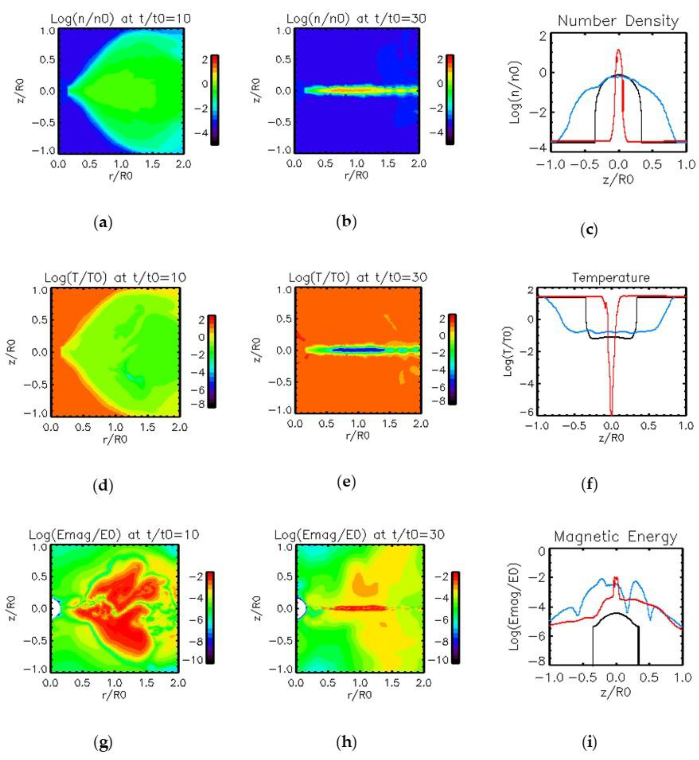
Figure 1 shows the results of Model 1. Upper panel shows the density distribution. Middle panel is the distribution of temperature. Lower panel shows the distribution of magnetic energy density. Left column is distribution at $t/t_0=10$. The initial torus and magnetic field evolve and mass accretion proceeds. After 10 rotations at the fiducial radius $r/R_0=1$, the hot accretion flow formed is geometrically thick and has the low density. It is regarded as ADAF. Middle column is the distribution of physical quantities at $t/t_0=30$. After radiative cooling is included, the accretion flow begins to condense and settle down to the midplane ($z/R_0=0$). Hot component of ADAF disappears by $t/t_0=15$. After that, the hot corona and the cool accretion disk co-exist. The temperature and density of the cool disk is about $T\sim {10}^{-6}{T}_0\sim 3\times {10}^5\hspace{0.17em}\mathrm{K}$ and $n\sim 10n_0\sim 5\times {10}^{19}{\mathrm{cm}}^{-3}$ respectively. The interface between the cool disk and the hot corona has steep gradients of density and temperature. Right column shows the vertical distributions of density, temperature, and magnetic energy density at $t/t_0=30$ and of the radius $r/R_0=0.8$. Black lines show the initial distributions. Blue lines show the distribution at $t/t_0=10$. We can identify the geometrically thick ADAF whose density is low, and temperature is high. Red lines show the results at $t/t_0=30$. The density of cool accretion disk around the midplane increases. The cool accretion disk decreases the geometrical thickness. On the other hand, the temperature of the cool accretion disk decreases. The quasi-steady state is achieved in the cool accretion disk, where radiative cooling is balanced with heating by Joule heating and compression. There is the steep gradient of temperature. We expect that thermal conduction plays an important role. The region which has the large magnetic energy was confined into the cool accretion disk. In this region plasma beta become smaller than unity. The magnetic pressure is dominant in the cool accretion disk.

3.2. Results of Model 2

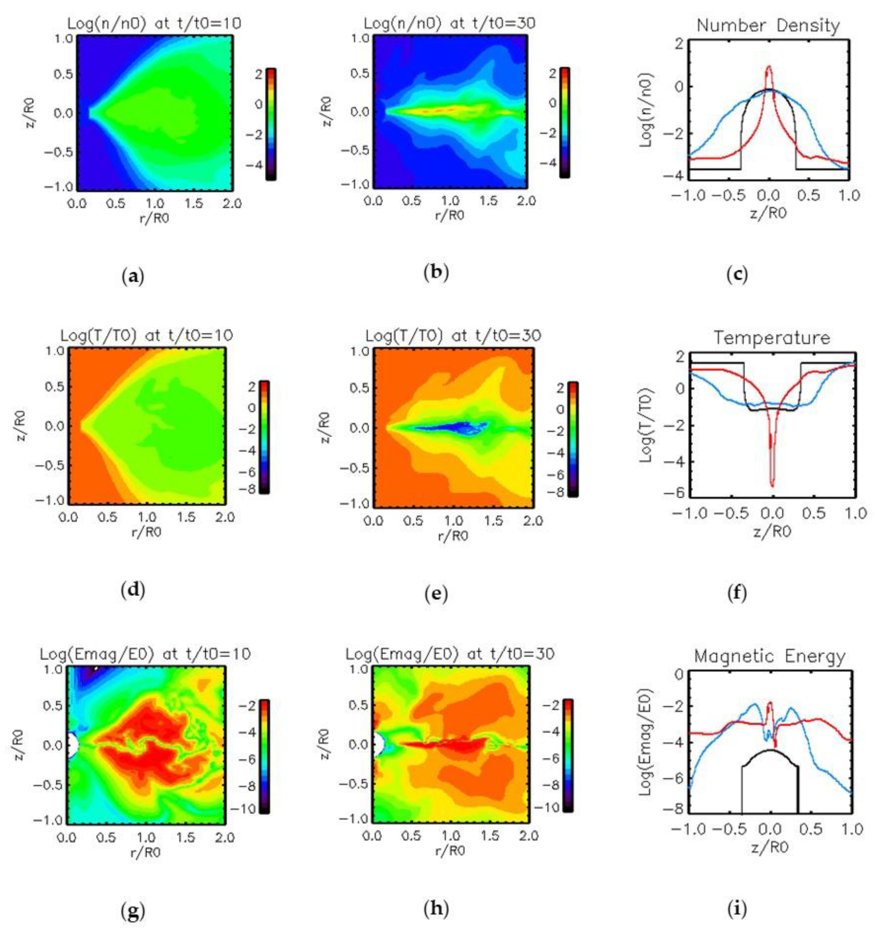
Figure 2 shows the results of Model 2 carried out by including thermal conduction. Upper, middle, and lower panels, and left, center, and right columns have same meaning as Figure 1. Although we include thermal conduction, almost the same hot accretion flow appears as Model 1. After the time passes $t/t_0=10$, the hot accretion flow condenses and produces a cool accretion disk inside. However, the hot accretion flow does not disappear perfectly in Model 2. The hot accretion flow changes its appearance to the intermediate region between the hot corona and the cool accretion disk. We see the sandwich structure of three components. The intermediate region becomes denser and has lower temperature than the corona surrounding the intermediate region. At this stage, the heat is transported from the corona to the cool accretion flow. Temporarily the cool accretion disk is formed; however, according to thermal conduction the disk partially evaporates gradually. In the intermediate region, magnetic field at $t/t_0=30$ is weaker than that at $t/t_0=10$; however it remains stronger than Model 1 at same time.

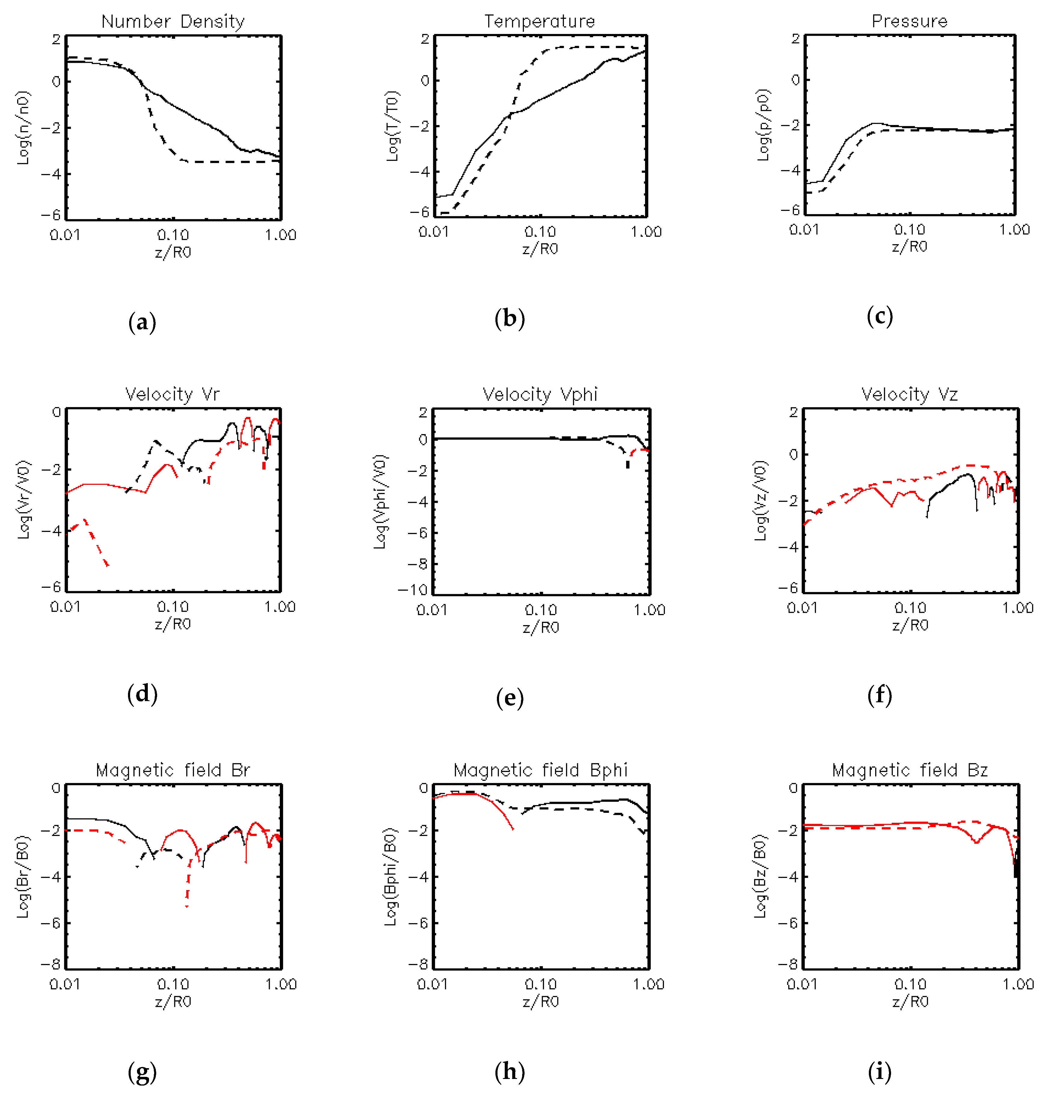
Figure 3 shows the vertical distributions of nine physical quantities averaged between $r/R_0=0.75$ and $r/R_0=0.85$ at $t/t_0=30$. Dashed and Solid lines represent the results of Model 1 and Model 2 respectively. Figure 3a–c show the number density, the temperature, and the pressure, respectively. The pressure does not vary very much in the intermediate region. Therefore, the density decreases with height ($\partial \ln n/\partial \ln z\sim -2$) in Model 2. Meanwhile, the temperature increases with height ($\partial \ln T/\partial \ln z\sim 2$).

In Model 1, the density and temperature show steep gradient. The difference between Model 1 and Model 2 indicate the existence of the intermediate region. The number density and temperature of the intermediate region are $5\times {10}^{15}<n\hspace{0.17em}[{\mathrm{cm}}^{-3}]<5\times {10}^{17}$ and $4\times {10}^{10}<T\hspace{0.17em}[\mathrm{K}]<4\times {10}^{12}$, respectively. The thickness of intermediate region is about $0.5R_0$. Figure 3d–f show the components of velocity. The azimuthal component of velocity simply shows the Keplerian rotation from the cool accretion disk to the outer corona. The radial and vertical components show the exchange of their signs. It means that there is inflow and outflow component of the intermediate region and the lower corona. Figure 3g–i show the vertical distributions of three components of magnetic field. Figure 3h shows that the azimuthal component of magnetic field is dominant. This has important meaning. If the magnetic field lines are wound tightly, it reduces the coefficient of thermal conduction in vertical direction. Effective optical depth integrated vertically is much smaller than unity, ${\tau }_{\mathrm{eff}}<0.052$ at $r/R_0=0.8$. The integration was done as follows:

$${\tau }_{\mathrm{eff}}={\displaystyle {\int }_{-10R_0}^{10R_0}\rho \sqrt{{\kappa }_{\mathrm{es}}{\kappa }_{\mathrm{ff}}}}dz,$$

(18)

where ${\kappa }_{\mathrm{es}}=0.34\hspace{0.17em}{\mathrm{cm}}^2{\mathrm{g}}^{-1}$ is the electron scattering opacity, ${\kappa }_{ff}=6.4\times {10}^{22}\rho T^{-7/2}{\mathrm{cm}}^2{\mathrm{g}}^{-1}$ is the free-free absorption opacity. The system that include intermediate region and cool accretion disk is optically thin enough.

4. Discussion

We solved the 2D MHD equations including the thermal conductivity. Previous works done by Das and Sharma, and Wu et al. are not MHD simulations but HD simulations using alpha viscous parameter [6,7]. We did not assume alpha viscosity. We assume that the angular momentum is transported mainly by the $r\phi$ element of the magnetic stress in the rotating gas. We define viscous alpha parameter ${\alpha }_{\mathrm{MHD}}$ as

$${\alpha }_{\mathrm{MHD}}=\frac{\langle \frac{B_r{B}_{\phi }}{4\pi }\rangle }{\langle p\rangle }=\frac{{\displaystyle \underset{\mathrm{Domain}}{\iiint }\frac{B_r{B}_{\phi }}{4\pi }dV}}{{\displaystyle \underset{\mathrm{Domain}}{\iiint }pdV}},$$

(19)

where “Domain” is the region of integration, $0.4<r/R_0<1.2$, $0<\phi <2\pi$ and $-0.3<z/R_0<0.3$. Figure 4a shows the time evolution of viscous parameter ${\alpha }_{\mathrm{MHD}}$. Black and red lines show the results of Model 1 and Model 2, respectively. Before radiative cooling is included ($t/t_0<10$), both calculations exhibit the magnitude is around ${\alpha }_{\mathrm{MHD}}~0.01$. This is a typical value used in hot accretion flows [6,7]. There is no large difference between our alpha parameter and ones of previous works. Hot accretion flows do not have large difference between models with thermal conduction or not. After radiative cooling is taken into account, the cool and dense accretion disk appears and ${\alpha }_{\mathrm{MHD}}$ rises and drops in a short time. There is the maximum ${\alpha }_{\mathrm{MHD}}\sim 0.1$. In the early stage of transition, the magnetic field changes the structure drastically and azimuthal magnetic field becomes strong by condensation [5]. That is the reason parameter ${\alpha }_{\mathrm{MHD}}$ shows rapid variation. The evolution of alpha parameter is not considered in previous works. Further analysis of the angular momentum transportation will be done in future.

Figure 4b shows the evolution of the luminosity normalized by the Eddington luminosity $L_{Edd}=4\pi GM{m}_{\mathrm{p}}c/{\sigma }_T=1.26\times {10}^{39}\mathrm{erg}/\mathrm{s}$. Here $m_{\mathrm{p}}$ is the proton mass and ${\sigma }_T$ is the Thomson cross section. We calculate the luminosity as

$$L={\displaystyle \underset{\mathrm{Domain}}{\iiint }{Q}_{\mathrm{br}}dV}.$$

(20)

Where the “Domain” means the region as $0<r/R_0<10$, $0<\phi <2\pi$ and $-10<z/R_0<10$. Black and red lines show the results of Model 1 and Model 2, respectively, as well as Figure 4a. Despite the appearance of the intermediate region, there is no difference between Model 1 and Model 2. Since mainly the cool accretion disk plays a role of the radiation of bremsstrahlung, we cannot distinguish the two models.

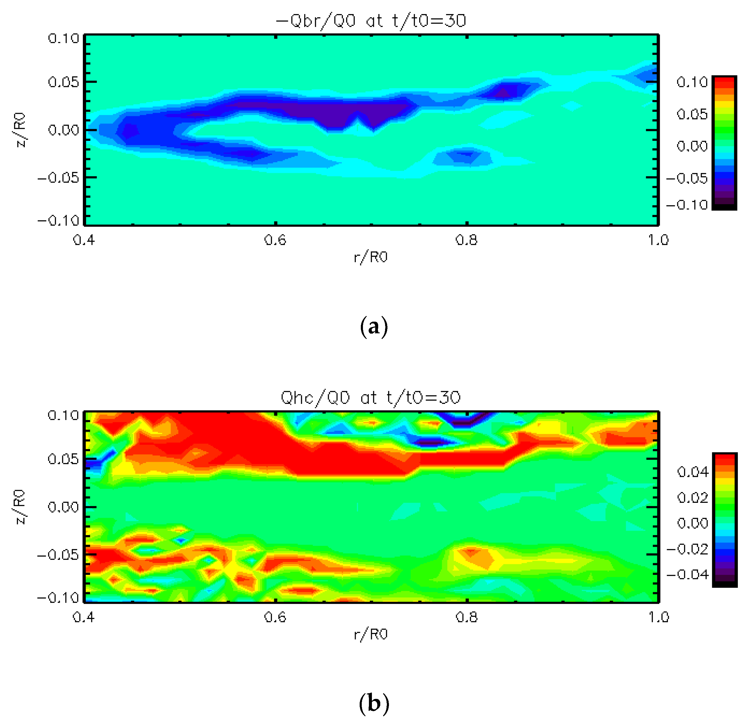
Figure 5a shows the radiative cooling rate of Model 2 at $t/t_0=30$. Region where radiative cooling is strong is localized in the cool accretion disk whose density is high. There is the temperature minimum at the midplane. Therefore, the radiative cooling rate at midplane become smaller than accretion flows around midplane. Figure 5b shows the thermal conduction rate of Model 2 at $t/t_0=30$. Thermal conduction works at the large temperature gradient. In this region $z/R_0\sim 0.05$, the vertical magnetic field is greater than the radial magnetic field (Figure 3d,f). Heat is transported from the intermediate region to the cool accretion disk effectively.

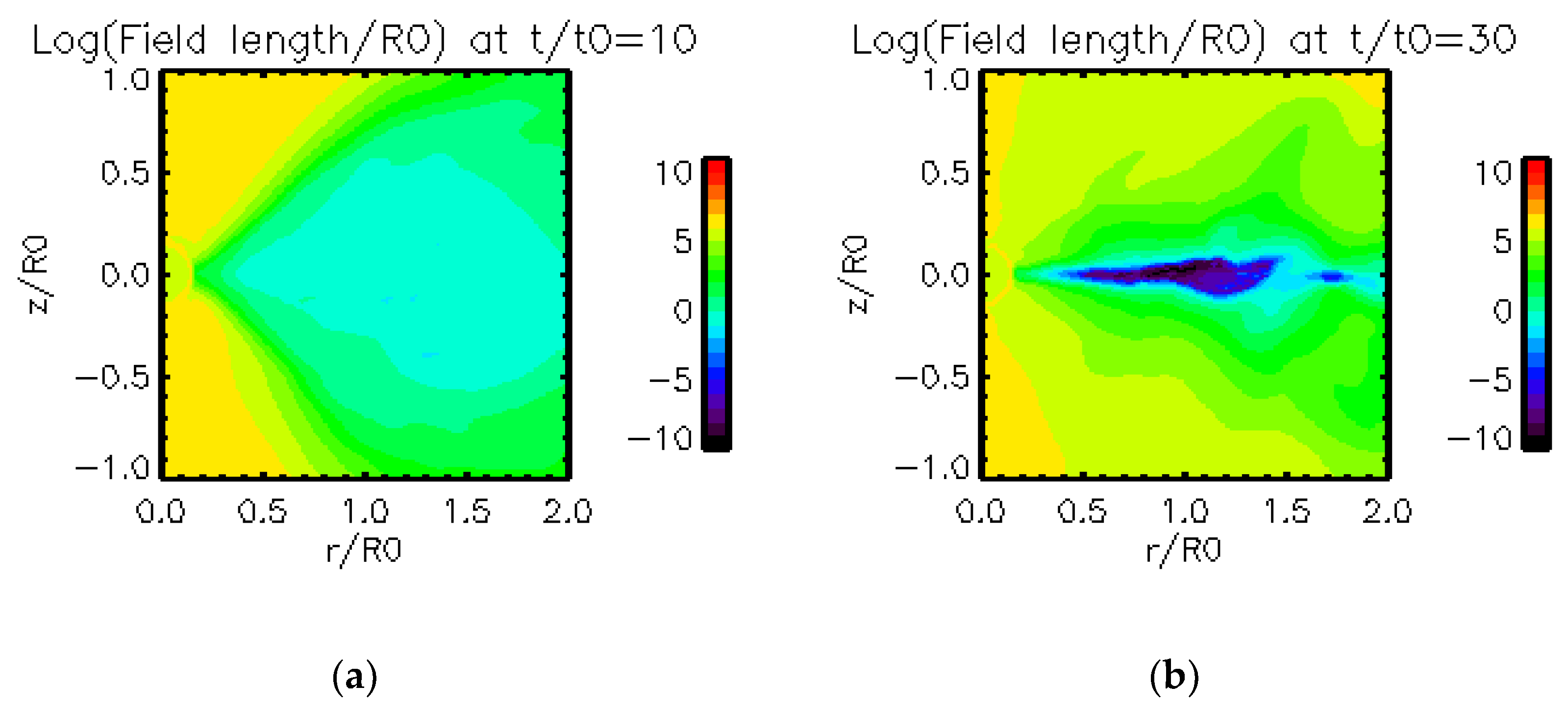
To compare the efficiency of thermal conduction and radiative cooling, we computed the Field length ${\lambda }_{\mathrm{F}}$ without including the heating term [24,25]. When the Field length is longer than the scale of the medium, thermal conduction dominates radiative cooling. On the other hand, when the Field length is shorter than the scale of the medium, radiative cooling dominates thermal conduction. Our numerical results show the magnetic field changes temporally and spatially in the $r-z$ plane. Since magnetic turbulence develops in the disk, we simply assume that heat conduction isotropic in the $r-z$ plane. The Field length computed without including the heating term is

$${\lambda }_F={\left[\frac{\kappa (T)T}{n^2{L}_M}\right]}^{\frac{1}{2}}={\left[\frac{6.0\times {10}^{-7}{T}^{\frac{5}{2}}T}{6.2\times {10}^{22}{\rho }^2{T}^{\frac{1}{2}}}\right]}^{\frac{1}{2}}=1.6\times {10}^8{\left[\frac{{\left(T/T_0\right)}^3}{{\left(\rho /{\rho }_0\right)}^2}\right]}^{\frac{1}{2}}\mathrm{cm}=5.3R_0{\left[\frac{{\left(T/T_0\right)}^3}{{\left(\rho /{\rho }_0\right)}^2}\right]}^{\frac{1}{2}}.$$

(21)

Figure 6a,b show the distribution of the Field length ${\lambda }_{\mathrm{F}}/R_0$ of Model 2 at $t/t_0=10$ and $t/t_0=30$, respectively. In the coronal region at $t/t_0=10$, since the Field length is longer than the size of the simulation region, thermal conduction dominates radiative cooling. However, in the region $r>z$, since radiative cooling becomes dominant over heat conduction, hot accretion flows can condensate by the cooling instability. On the other hand, thermal conduction suppresses the cooling instability in the intermediate region at $t/t_0=30$.

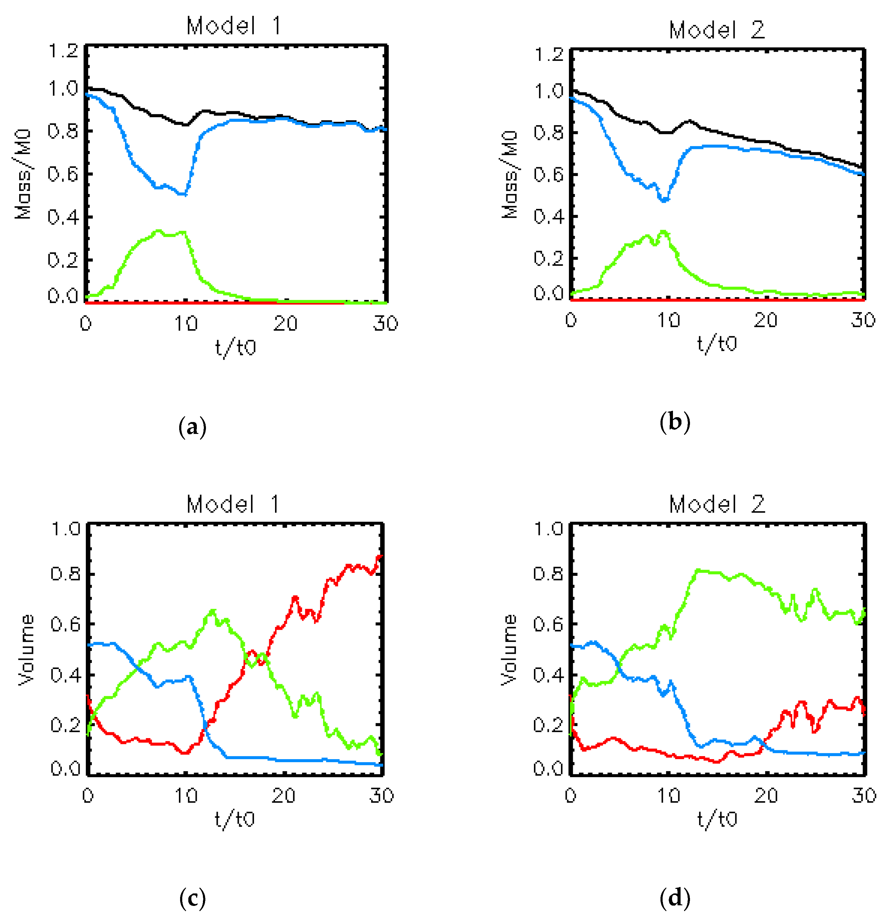
Figure 7 shows the evolutions of mass and volume whose medium is in three temperature ranges in the cylinder defined as $0<r/R_0<1.6$, $0<\phi <2\pi$ and $-1.6<z/R_0<1.6$ except for the sphere $\sqrt{r^2+z^2}/R_0<0.3$. Three temperature range are $T/T_0>10$ (denoted by red line), $0.1<T/T_0<10$ (denoted by green line) and $T/T_0<0.1$ (denoted by blue line), these temperature ranges are supposed to be the hot corona, the intermediate region and the cool accretion disk, respectively. Figure 7a,b show that the intermediate region remains by thermal conduction against radiative cooling. Although the mass of intermediate region is small compared to cool accretion disk, the volume of intermediate region is large compared to other temperature region (Figure 7c,d). These situations and sandwich structure of three components is helpful to produce the hard X-ray spectral component by inverse-Compton processes. Post process calculations by a Monte Carlo simulation for X-ray spectrum will be presented in subsequent papers.

In this study, we considered radiative cooling by bremsstrahlung. Synchrotron radiation and inverse-Compton scattering can change the structure of accretion disks in the equatorial region and the intermediate region. Das and Sharma pointed out the possibility that synchrotron radiation and inverse-Compton scattering have same dependency on the density as bremsstrahlung [6]. We think that increase of the density may compensate the lack of radiative cooling. When we consider radiative cooling by synchrotron radiation and inverse-Compton scattering, the formed cool accretion disk has lower temperature and higher number density than the results of our present study. Inverse-Compton scattering reduces the thickness of the intermediate region. On the other hand, thermal conduction suppresses the shrinks of the intermediate region. We will perform the parameter survey of density in future.

We set the upper limit of temperature to evaluate the coefficient of thermal conductivity, since we solve one-temperature MHD equations. We suppose that the upper limit of temperature is electron temperature in two-temperature accretion flows [2]. It is also useful to avoid the unusual thermal conductivity in high-temperature and low-density corona. As is well known, ADAFs has the two-temperature structures. The electron temperature is suppressed to be lower than the ion temperature since the energy exchange rate between ions and electrons by the Coulomb coupling is low due to the low density and the short free-fall time scale. It is preferable to simulate the two-temperature MHD to consider the state transition when the intermediate region exists. Wu et al. consider the two-temperature HD models; however, they do not calculate the two energy equations for ions and electrons independently [7]. We are seeking to update our codes which solve two-temperature MHD equations.

The state transition is driven by the variation of the mass accretion rate. However, we do not include the mass supply calculation in our codes. We studied the various initial condition of density, $1.0\times {10}^{-8}<{\rho }_0\hspace{0.17em}[{\mathrm{g}/\mathrm{cm}}^3]<1.0\times {10}^{-4}$. Instead of the mass supply, we choose the critical initial condition of the density which can make the hot accretion flow condense. It is easy to obtain the results of the MHD simulation of the state transition. Machida et al. and Wu et al. adopt this concept [5,7]. However, it is preferable to implement the subroutine of the mass supply to achieve the cycle of the state transition in simulations by controlling the mass accretion rate [6]. This difficulty should be solved in future.

References

- Remillard, R.A.; McClintock, J.E. X-ray properties of black-hole binaries. Ann. Rev. Astron. Astrophys. 2006, 44, 49–92. [Google Scholar] [CrossRef]
- Narayan, R.; Yi, I. Advection-dominated accretion: Underfed black holes and neutron stars. Astrophys. J. 1995, 452, 710–735. [Google Scholar] [CrossRef]
- Abramowicz, M.A.; Chen, X.; Kato, S.; Lasota, J.P.; Regev, O. Thermal equilibria of accretion disks. Astrophys. J. 1995, 438, L37–L39. [Google Scholar] [CrossRef]
- Shakura, N.I.; Sunyaev, R.A. Black holes in binary systems. Observational Appearance. Astron. Astrophys. 1973, 24, 337–355. [Google Scholar]
- Machida, M.; Nakamura, K.E.; Matsumoto, R. Formation of magnetically supported disks during hard-to-soft transitions in black hole accretion flows. Publ. Astron. Soc. Jpn. 2006, 58, 193–202. [Google Scholar] [CrossRef]
- Das, U.; Sharma, P. Radiatively inefficient accretion flow simulations with cooling: Implications for black hole transitions. Mon. Not. R. Astron. Soc. 2013, 435, 2431–2444. [Google Scholar] [CrossRef]
- Wu, M.C.; Xie, F.G.; Yuan, Y.F.; Gan, Z. Hot Accretion flow with radiative cooling: State transitions in black hole X-ray binaries. Mon. Not. R. Astron. Soc. 2016, 459, 1543–1553. [Google Scholar] [CrossRef]
- Balbus, S.A.; Hawley, J.F. A powerful local shear instability in weakly magnetized disks I. Linear analysis. Astrophys. J. 1991, 376, 214–222. [Google Scholar] [CrossRef]
- Hawley, J.F.; Balbus, S.A. A powerful local shear instability in weakly magnetized disks II. Nonlinear evolution. Astrophys. J. 1991, 376, 223–233. [Google Scholar] [CrossRef]
- Yokoyama, T.; Shibata, K. Magnetic reconnection coupled with heat conduction. Astrophys. J. 1997, 474, L61–L64. [Google Scholar] [CrossRef]
- Yokoyama, T.; Shibata, K. A two-dimensional magnetohydrodynamic simulation of chromosphereic evaporation in a solar flare based on a magnetic reconnection model. Astrophys. J. 1998, 494, L113–L116. [Google Scholar] [CrossRef]
- Yokoyama, T.; Shibata, K. Magnetohydrodynamic simulation of a solar flare with chromosphereic evaporation effect based on the magnetic reconnection model. Astrophys. J. 2001, 549, 1160–1174. [Google Scholar] [CrossRef]
- Isobe, H.; Shibata, K.; Yokoyama, T.; Imanishi, K. Hydrodynamic Modeling of a Flare Loop Connecting the Accretion Disk and Central Core of Young Stellar Objects. Publ. Astron. Soc. Jpn 2003, 55, 967–980. [Google Scholar] [CrossRef] [Green Version]
- Meyer, F.; Meyer-Hofmeister, E. Accretion disk evaporation by a coronal siphon flow. Astron. Astrophys. 1994, 288, 175–182. [Google Scholar]
- Meyer-Hofmeister, E.; Meyer, F. The effect of heat conduction on the interaction of disk and corona around black holes. Astron. Astrophys. 2006, 449, 443–447. [Google Scholar] [Green Version]
- CANS (Coordinated Astronomical Numerical Software). Available online: http://www-space.eps.s.u-tokyo.ac.jp/~yokoyama/etc/cans/index-e.html (accessed on 31 October 2018).
- Van der Vorst, H.A. Bi-CGSTAB: A fast and smoothly converging variant of Bi-CG for the solution of Nonsysmmetric Linear Systems. SIAM J. Sci. Stat. Comput. 1992, 13, 631–644. [Google Scholar] [CrossRef]
- Templates. Available online: http://www.netlib.org/templates/double/ (accessed on 23 December 2018).
- Pacyńsky, B.; Wiita, P.J. Thick accretion disks and supercritical luminosities. Astron. Astrophys. 1980, 88, 23–31. [Google Scholar]
- Priest, E.R. Solar Magnetohydrodynamics; D. Reidel Publishing Company: Dordrecht, The Netherlands, 1982; pp. 84–91. ISBN 9027718834. [Google Scholar]
- Shukurov, A. Introduction to galactic dynamos. In Mathematical Aspects of Natural Dynamos; Dormy, E., Soward, A.M., Eds.; Taylor and Francis: New York, NY, USA, 2007; pp. 319–366. ISBN 9781420055269. [Google Scholar]
- Oliver, G.; Elstner, D.; Ziegler, U. Towards a hybrid dynamo model for the Milky Way. Astron. Astrophys. 2013, 560, A93. [Google Scholar]
- Papaloizou, J.C.B.; Pringle, J.E. The dynamical stability of differentially rotating discs with constant specific angular momentum. Mon. Not. R. Astron. Soc. 1984, 208, 721–750. [Google Scholar] [CrossRef] [Green Version]
- Field, G.B. Thermal instability. Astrophys. J. 1965, 142, 531–567. [Google Scholar] [CrossRef]
- Begelman, M.C.; McKee, C.F. Global effects of thermal conduction on two-phase media. Astrophys. J. 1990, 358, 375–391. [Google Scholar] [CrossRef]
Figure 1.
Results of Model 1. (a) Distribution of number density at before cooling term is included. (b) Distribution of number density at . (c) Vertical distribution of number density at three different time and at . Black line shows initial condition at . Blue line shows result at . Red line shows result at . (d) Distribution of temperature at . (e) Distribution of temperature at . (f) Vertical distribution of temperature. Color scale is the same as (c). (g) Distribution of magnetic energy density at . (h) Distribution of magnetic energy density at . (i) Vertical distribution of magnetic energy density. Colors have the same meaning as (c) and (f).
Figure 2.
Results of Model 2. Same quantities and conditions of visualization as Figure 1.
Figure 3.
Results of Model 1 and Model 2 at . Dashed lines represent the result of Model 1. Solid Lines represent the results of Model 2. These panels show the vertical distributions of the nine physical quantities averaged between and . Black lines indicate positive values. Red lines indicate negative values, that is, mean the absolute values of quantities. (a) Number density. (b) Temperature. (c) Pressure. (d) Radial component of velocity. (e) Azimuthal component of velocity. (f) Vertical component of velocity. (g) Radial component of magnetic field. (h) Azimuthal component of magnetic field. (i) Vertical component of magnetic field.
Figure 4.
Evolutions of the averaged magnetic stress and integrated luminosity. Black lines show the results of Model 1 without thermal conduction. Red lines show the results of Model 2 including thermal conduction. (a) Averaged viscous alpha parameter . Integration is done in the domain of , and . (b) Integrated luminosity normalized by the Eddington luminosity. Integration is done in the domain of , and excluding the region of . Colors denote same meaning as (a).
Figure 5.
(a) Distributions of radiative cooling rate of Model 2 at . is normalization unit. (b) Distributions of thermal conduction rate at .
Figure 6.
Distributions of the Field length of Model 2. (a) Result at (b) Result at .
Figure 7.
Time evolution of mass and volume of Model 1 and Model 2. Results are obtained by the integration in the domain of , and except for the region of . These are normalized by initial total mass and volume of the above domain, respectively. (a) Model 1. Blue line shows the mass of gas whose temperature range is . Green line shows the mass of . Red line shows the mass of . Black line shows sum of three components. (b) Model 2. Same as (a). (c) Model 1. Time evolution of volume of each temperature range same as (a). Colors mean same as (a). (d) Model 2. Same as (c).