Distribution and Evolution of Metals in the Magneticum Simulations

Abstract

Metals are ideal tracers of the baryonic cycle within halos. Their composition is a fossil record connecting the evolution of the various stellar components of galaxies to the interaction with the environment by in- and out-flows. The Magneticum simulations allow us to study halos across a large range of masses and environments, from massive galaxy clusters containing hundreds of galaxies, down to isolated field galaxies. They include a detailed treatment of the chemo-energetic feedback from the stellar component and its evolution, as well as feedback from the evolution of supermassive black holes. Following the detailed evolution of various metal species and their relative composition due to continuing enrichment of the IGM and ICM by SNIa, SNII and AGB winds of the evolving stellar population is revealed the complex interplay of local star-formation processes, mixing, global baryonic flows, secular galactic evolution and environmental processes. We present results from the Magneticum simulations on the chemical properties of simulated galaxies and galaxy clusters, carefully comparing them to observations. We show that the simulations already reach a very high level of realism within their complex descriptions of the chemo-energetic feedback, successfully reproducing a large number of observed properties and scaling relations. Our simulated galaxies clearly indicate that there are no strong secondary parameters (such as star-formation rates at a fixed redshift) driving the scatter in these scaling relations. The remaining differences clearly point to detailed physical processes, which have to be included in future simulations.

1. Introduction

In cosmological hydrodynamical simulations, star formation is typically treated as based on a sub-grid model. Star particles are formed when the gas locally exceeds a certain density threshold, when it is Jeans unstable, and the local gas flow converges at a gas particle. Each star particle represents a simple stellar population that is characterized by an initial mass function (IMF).

In addition, each star particle emits a feedback that mimicks the winds that are launched by stars in reality by averaging over the whole stellar population included in each simulated stellar particle. In most models, the considered winds are composed of three main stellar sources: supernovae Type II (SNII), supernovae Type Ia (SNIa), and asymptotic giant branch (AGB) stars. These three sources are considered to be the most important drivers of observed stellar outflows and thus the main contributors to metal enrichment of the interstellar medium.

Stars with masses larger than 8 $M_{\odot }$ are believed to end their lives through a “core collapse” (SNII), typically releasing an energy of ${10}^{51}$ erg per supernova together with their chemical imprint into the surrounding gas. These supernovae usually occur shortly after the formation of the simulated star particle, as the most massive stars only live for a short time, and thus this part of the stellar population of the star particle emits first. SNIa, on the other hand, are believed to arise from thermonuclear explosions of white dwarfs within binary stellar systems. These supernovae are delayed relative to the SNII and occur later in a star particle’s life, as the white dwarf in the according binary system has to first be formed, and second, needs to accrete matter from its companion until it reaches the mass threshold for the onset of thermonuclear burning. Therefore, a detailed modeling of the evolution of the stellar population has to be included in the simulations to follow the chemo-energetic imprint of the SNIa on the surrounding gas. AGB stars contribute emitting strong winds, exhibiting strong mass losses during their life and importantly contribute to the nucleosynthesis of heavy elements.

To include the effects of these sources in the sub-grid models of simulated stellar particles raises the need to integrate a set of complicated equations describing the evolution of a simple stellar population. Such a set of integral equations then allows us to compute at each time the rate at which the current AGB stars pollute their environment by stellar winds and the rate at which the SNIa and SNII are exploding. Therefore they allow us to properly treat the chemo-energetic imprint on the surrounding inter-galactic medium (IGM) and the inter-cluster medium (ICM). In the following, we will give a short, schematic description of such calculations on the basis of the description presented by Dolag et al., 2017 [1] (for a more detailed review, see Matteucci, 2003 [2] and Borgani et al., 2008 [3], and references therein). Then we will introduce the cosmological hydrodynamical simulation set used in this work, and present a comparison of the metal enrichment in galaxies and clusters of galaxies caused by this model feedback, along with observations. Finally, we will summarize and discuss the results of this comparison in the light of model improvements needed for the future.

2. Chemical Enrichment

To describe the continuous enrichment of the IGM and ICM through winds from SNIa, SNII and AGB stars in the evolving stellar population of each star particle, several ingredients are needed. In the following, we will shortly present the ingredients used in many state-of-the-art cosmological simulations of galaxy formation.

2.1. Initial Mass Function

One of the most important quantities in models of chemical evolution is the IMF. It directly determines the relative ratio between SNII and SNIa, and therefore the relative abundance of $\alpha$-elements and Fe-peak elements. The shape of the IMF also determines the ratio between low-mass long-living and massive short-living stars. This ratio directly affects the amount of energy released by the SNe, as well as the present luminosity of galaxies, which is dominated by low-mass stars and the (metal) mass-locking in the stellar phase.

The IMF $\varphi \left(m\right)$ describes the number of stars of a given mass per unit logarithmic mass interval. Historically, a commonly used form is the Salpeter IMF (Salpeter, 1955 [4]), which follows a single power-law with an index of $x=1.35$. However, different expressions of the IMF have been proposed more recently in order to model a flattening in the low-mass regime of the stellar mass function that is currently favoured by a number of observations. Among the newer, often-used models is the Chabrier IMF (Chabrier, 2003 [5]), which has a continuously changing slope and is more top-heavy than the Salpeter IMF:

$$\varphi \left(m\right)\propto \left\{\begin{array}{cc}{m}^{-1.3}\hfill & m>1{\mathrm{M}}_{\odot }\hfill \\ \hfill \\ e^{\frac{-{\left(log\left(m\right)-log\left(m_c\right)\right)}^2}{2{\sigma }^2}}\hfill & m\le 1{\mathrm{M}}_{\odot }\hfill \end{array}\right.$$

(1)

However, the questions of whether there is a global IMF or if the IMF is changing with galaxy mass, morphology or cosmological time, and which IMF has to be chosen, are still unsolved problems and matters of heavy debate.

2.2. Lifetime Functions

To model the evolution of a simple stellar population, a detailed knowledge of the lifetimes of stars with different masses is required. Different choices for the mass-dependence of the lifetime function have been proposed in the literature (e.g., Padovani and Matteucci, 1993 [6]; Maeder and Meynet, 1989 [7]; Chiappini et al., 1997 [8]), where the latest reads:

$$\tau \left(m\right)=\left\{\begin{array}{cc}{10}^{-0.6545logm+1}\hfill & m\le 1.3{\mathrm{M}}_{\odot }\hfill \\ \hfill \\ {10}^{-3.7logm+1.351}\hfill & 1.3<m\le 3{\mathrm{M}}_{\odot }\hfill \\ \hfill \\ {10}^{-2.51logm+0.77}\hfill & 3<m\le 7{\mathrm{M}}_{\odot }\hfill \\ \hfill \\ {10}^{-1.78logm+0.17}\hfill & 7<m\le 15{\mathrm{M}}_{\odot }\hfill \\ \hfill \\ {10}^{-0.86logm-0.94}\hfill & 15<m\le 53{\mathrm{M}}_{\odot }\hfill \\ \hfill \\ 1.2\times m^{-1.85}+0.003\hfill & \mathrm{otherwise}.\hfill \end{array}\right.$$

(2)

2.3. Stellar Yields

The ejected masses of the different metal species i produced by a star of mass m are called stellar yields p${}_{Z_i}$(m,Z). These yields depend on the metallicity Z with which the star originally formed, and on the type of outflow ejected from the star. Therefore, detailed predictions for the main three sources of enrichment are needed, namely for the mass loss of AGB stars, of SNII, and of SNIa. To date, such predictions still suffer from significant uncertainties, mainly due to the still poorly understood mass loss through stellar winds in stellar evolution models, which depends on multiple additional physical processes.

For the mass loss through AGB stars, the most recent predictions can be found in Karakas, 2007 [9]. Predictions for the mass loss from massive stars driving SNII are presented by Nomoto, Kobayashi & Tominaga, 2013 [10]. The most complete table for SNIa to date is presented by Thielmann, 2003 [11].

2.4. Modeling the Enrichment Process

As summarized by Dolag, 2017 [1], the assumption of a generic star-formation history represented by an arbitrary function of time $\psi \left(t\right)$ allows us to compute the rates for the different contributions in the form of a set of integral equations as shown in the following (for more details, see also Matteucci, 2003 [2], Borgani et al., 2008 [3], and references therein). This formalism can be individually applied to the large number of particles representing the continuous star-formation process within cosmological simulations. Every star particle here represents a stellar population born in a single burst. The combination of all the stellar components within the simulated galaxies then results in a model that describes the legacy of the detailed star-formation history of any simulated galaxy.

2.4.1. Type Ia Supernovae

SNIa occur in binary systems with masses in a mass range of 0.8–8 M${}_{\odot }$. Letting $m_{\mathrm{B}}$ be the total mass of the binary system and $m_2$ be the mass of the secondary companion, we can now use $f\left(\mu \right)$ as the distribution function of binary systems with $\mu =m_2/m_{\mathrm{B}}$, and define A as the fraction of stars in binary systems that are progenitors of SNIa. Therefore, A has to be given or be obtained by a model. Constructing such detailed models for SNIa progenitors is particularly difficult; see, for example, Greggio & Renzini, 1983 [12] or Greggio, 2005 [13]. On the basis of such kinds of models, typical values for A are inferred to be in the range from $0.05$ to $0.1$, on the basis of comparisons of chemical enrichment models with observed iron metallicities within galaxy clusters (e.g., Matteucci & Gibson, 1995 [14]) or within the solar neighbourhood (e.g., Matteucci & Greggio, 1986 [15]). Within the current simulations we are using a value of $A=0.1$. With these ingredients and the mass-dependent lifetime functions $\tau \left(m\right)$, we can model the rate of SNIa as

$$R_{\mathrm{SN}\mathrm{Ia}}\left(t\right)=A\underset{{\displaystyle M_{\mathrm{B},\inf }}}{\overset{{\displaystyle M_{\mathrm{B},\sup }}}{\int }}\varphi \left(m_{\mathrm{B}}\right)\underset{{\displaystyle {\mu }_{\mathrm{m}}}}{\overset{{\displaystyle {\mu }_{\mathrm{M}}}}{\int }}f\left(\mu \right)\psi (t-{\tau }_{m_2})\mathrm{d}\mu \mathrm{d}{m}_{\mathrm{B}}$$

(3)

where $M_{\mathrm{Bm}}$ and $M_{\mathrm{BM}}$ are the smallest and largest values, respectively, that are allowed for the progenitor binary mass $m_{\mathrm{B}}$. Then, the integral over $m_{\mathrm{B}}$ runs in the range between $M_{\mathrm{B},\inf }$ and $M_{\mathrm{B},\sup }$, which represent the minimum and the maximum value of the total mass of the binary system that is allowed to explode at the time t. These values in general are functions of $M_{\mathrm{Bm}}$, $M_{\mathrm{BM}}$, and $m_2\left(t\right)$, which in turn depend on the star-formation history $\mathsf{\Psi }\left(t\right)$. In simulations, where the individual stellar particles are commonly modeled as an impulsive star-formation event, $\psi \left(t\right)$ can therefore be approximated with a Dirac $\delta$-function. The sum of all stellar particles and their individual formation time then represent the complex star-formation history of the galaxies within the simulation.

2.4.2. Supernovae Type II, Low-, and Intermediate-Mass Stars

Computing the rates of SNII, low-mass stars (LMS), and intermediate-mass stars (IMS) is conceptually simpler than calculating the rates of SNIa, as they are purely driven by the lifetime function $\tau \left(m\right)$ convolved with the star-formation history $\psi \left(t\right)$ and multiplied by the IMF $\varphi (m={\tau }^{-1}\left(t\right))$. Because $\psi \left(t\right)$ is a delta-function for the simple stellar populations used in simulations, the SNII, LMS and IMS rates read

$$R_{\mathrm{SNII}\left|\mathrm{LMS}\right|\mathrm{IMS}}\left(t\right)=\varphi \left(m\left(t\right)\right)\times \left(-\frac{dm\left(t\right)}{dt}\right)$$

(4)

where $m\left(t\right)$ is the mass of the star that dies at time t. For AGB rates, the above expression must be multiplied by a factor of $(1-A)$ if the mass $m\left(t\right)$ falls in the range of masses, which is relevant for the secondary stars of SNIa binary systems.

2.4.3. The Equations of Chemical Enrichment

In order to compute the total metal release from the simple stellar population, we have to fold the above rates with the yields $p_{Z_i}^{\mathrm{SNIa}\left|\mathrm{SNII}\right|\mathrm{AGB}}(m,Z)$ from SNIa, SNII and AGB stars for a given element i for stars born with initial metallicity $Z_i$, and compute the evolution of the density ${\rho }_i\left(t\right)$ for each element i at each time t. As shown by Borgani et al., 2008 [3], this reads

$$\begin{array}{ccc}\hfill {\dot{\rho }}_i\left(t\right)=& -& \psi \left(t\right)Z_i\left(t\right)\hfill \end{array}$$

(5)

$$\begin{array}{cc}+& {\int }_{M_{BM}}^{M_U}\psi (t-\tau \left(m\right))p_{Z_i}^{\mathrm{SNII}}(m,Z)\phi \left(m\right)dm\hfill \end{array}$$

(6)

$$\begin{array}{cc}+& A{\int }_{M_{Bm}}^{M_{BM}}\varphi \left(m\right)\left[{\int }_{{\mu }_{\mathrm{m}}}^{{\mu }_{\mathrm{M}}}f\left(\mu \right)\psi (t-{\tau }_{m_2})p_{Z_i}^{\mathrm{SNIa}}(m,Z)d\mu \right]dm\hfill \end{array}$$

(7)

$$\begin{array}{cc}+& (1-A){\int }_{M_{Bm}}^{M_{BM}}\psi (t-\tau \left(m\right))p_{Z_i}^{\mathrm{AGB}}(m,Z)\phi \left(m\right)dm\hfill \end{array}$$

(8)

$$\begin{array}{cc}+& {\int }_{M_L}^{M_{Bm}}\psi (t-\tau \left(m\right))p_{Z_i}^{\mathrm{AGB}}(m,Z)\phi \left(m\right)dm\hfill \end{array}$$

(9)

where $M_{\mathrm{L}}$ and $M_{\mathrm{U}}$ are the minimum and maximum mass of a star in the simple stellar population, respectively. Commonly adopted choices for these limiting masses are $M_{\mathrm{L}}\simeq 0.1$ M${}_{\odot }$ and $M_{\mathrm{U}}\simeq 100$ M${}_{\odot }$.

In the above equation, the first line describes the locking of metals in newborn stars through the currently ongoing star formation $\psi \left(t\right)$, which, for the assumed sub-grid model case, vanishes as $\psi \left(t\right)$ is a delta-function. For a comprehensive review of the analytic formalism we refer the reader to Greggio, 2005 [13].

3. The Magneticum Simulations

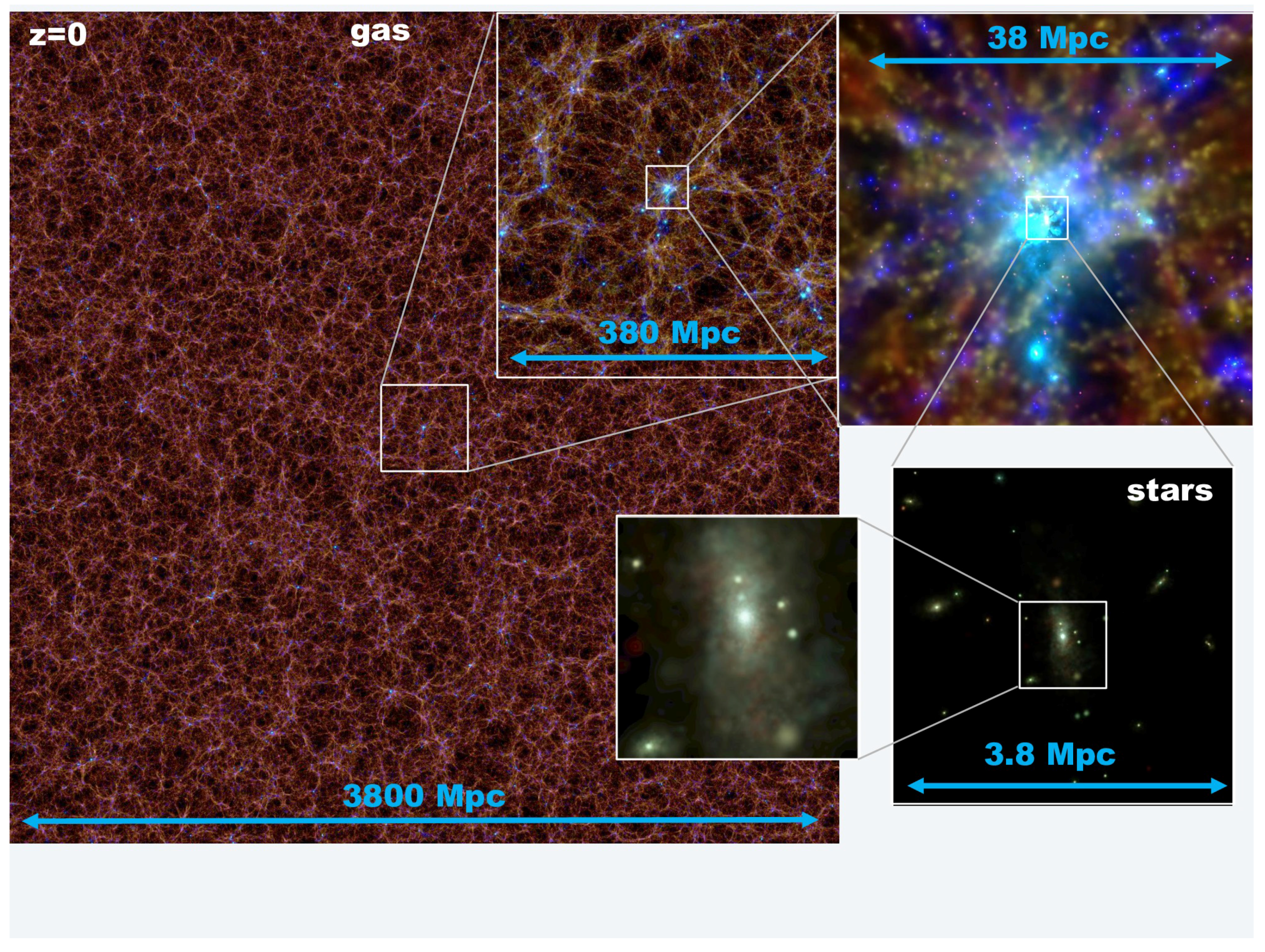
The Magneticum simulation set covers a huge dynamical range, from very large cosmological volumes as shown in Figure 1, which can be used for statistical studies of clusters and voids (e.g., Bocquet et al., 2016 [16], Pollina et al., 2017 [17]), to very high-resolution simulations of smaller cosmological volumes, which allow for a morphological classification and a detailed analysis of galaxies and their properties (e.g., Teklu et al., 2015 [18], Remus et al., 2017 [19]).

Table 1. Size and number of particles for the different simulations. The last two rows list the average mass and softening of the star particles for the different resolution levels.

Simulation	Box0	Box1	Box2b	Box2	Box3	Box4	${\mathit{m}}_{\mathbf{star}}$	${\mathit{ϵ}}_{\mathbf{star}}$
Size [Mpc]	3820	1300	910	500	180	68	[${\mathit{M}}_{\mathbf{\odot }}\mathbf{/}\mathit{h}$]	[kpc/h]
mr	$2\times {4536}^3$	$2\times {1512}^3$	–	$2\times {594}^3$	$2\times {216}^3$	$2\times {81}^3$	$4.7\times {10}^8$	5
hr	–	–	$2\times {2880}^3$	$2\times {1564}^3$	$2\times {576}^3$	$2\times {216}^3$	$2.6\times {10}^7$	2
uhr	–	–	–	–	$2\times {1536}^3$ (z = 2)	$2\times {576}^3$	$1.3\times {10}^6$	0.7

lists the detailed properties, such as size and stellar mass-resolution, of the different simulations. These simulations treat the metal-dependent radiative cooling, heating from a uniform time-dependent ultraviolet background, star formation and the chemo-energetic evolution of the stellar population as traced by SNIa, SNII and AGB stars with the associated feedback processes and stellar evolution details described before. They also include the formation and evolution of supermassive black holes and the associated quasar and radio-mode feedback processes. For a detailed description of the simulation sample, see Dolag et al., (in prep); Hirschmann et al., 2014 [20]; and Teklu et al., 2015 [18].

4. Metallicities from Magneticum in Comparison to Observations

As previously shown from re-simulations of massive galaxy clusters, the observed radial profiles of iron within the ICM can be well reproduced in simulations: Biffi et al., 2017, [21] demonstrated that, especially at high redshifts, the implemented AGN feedback is the main driver for enhancing the metal enrichment in the ICM at large cluster-centric distances to the observed level.

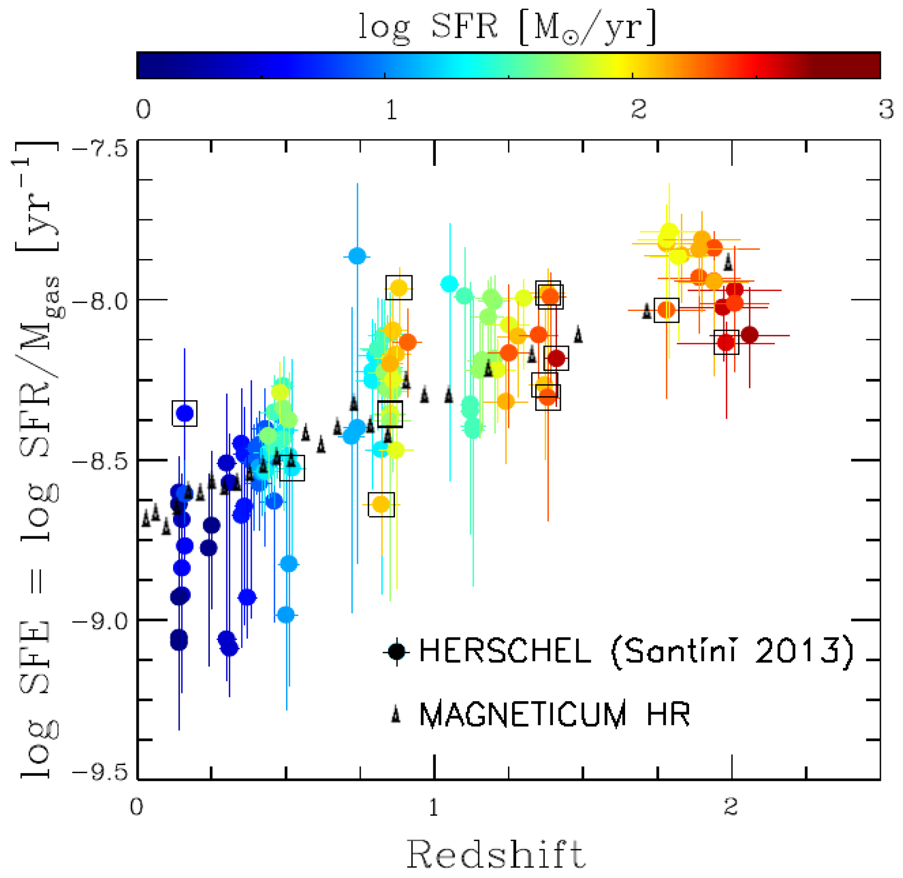
The Magneticum simulations now allow such investigations across a much larger range of halo masses. For this study, we use a large simulation volume (Box2 hr) with enough resolution to resolve mean properties of galaxies (and AGNs), resulting in the same resolution as used by Biffi et al., 2017 [21] and Hirschmann et al., 2014 [20]. For galaxies, the star-formation efficiency (SFE) is a measure of the SFR per unit of gas mass. To evaluate whether the SF activity in the simulations matches the observational data is a key step to proceed towards reproducing the observed mass–metallicity relation (MZR). In Figure 2, the evolution of the observed SFE up to a redshift of $z\approx 2$ is shown in comparison to the evolution of the SFE of star-forming galaxies in Magneticum. As can clearly be seen, the simulations are in excellent agreement with the observed trends up to $z\approx 2$.

4.1. Galaxy Clusters: ICM Metallicities

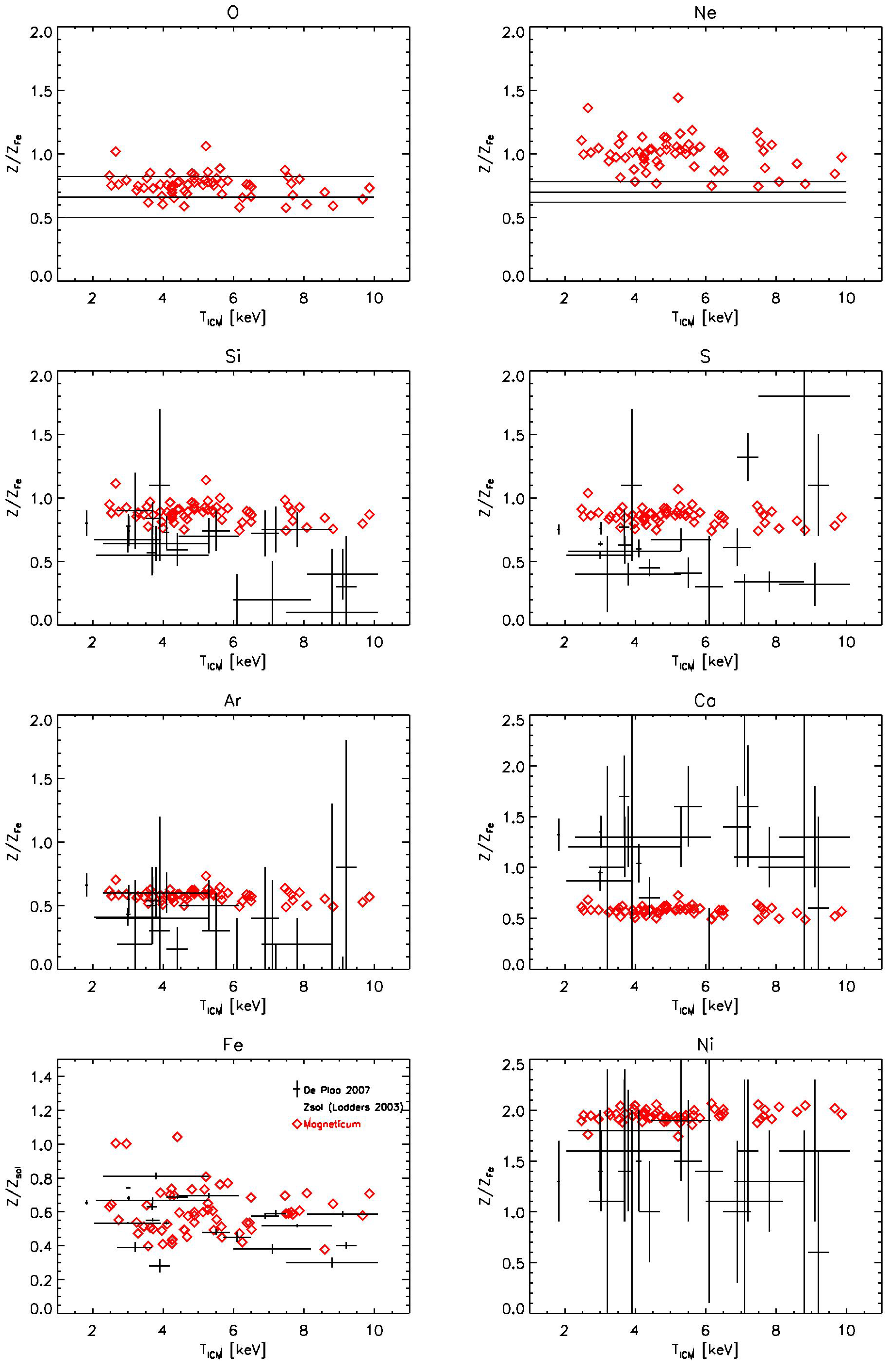
X-ray observations of the intracluster medium allow for a detailed study of the distribution of different metal species within the ICM via their line emissions within the X-ray band. Here, the composition of the individual metal species allows us to interpret their abundances as an imprint of the relative contributions to the enrichment from SNIa and SNII, hence keeping a record on when and where these metals are injected into the ICM (e.g., De Plaa et al., 2007 [23]). The lower left panel of Figure 3 shows a comparison of such observational data for various individual galaxy clusters using simulations, clearly demonstrating the ability of the Magneticum simulations to reproduce the correct absolute iron abundance within the ICM self-consistently.

Here, the scattering of the absolute iron abundance within the simulated clusters shows a similar spread (factor of two) as the observed values, and a very mild trend of increasing iron abundance for low-mass (e.g., lower ICM temperature) clusters. In addition, the simulations also broadly reproduce the chemical composition footprint of various elements’ species, as shown in the various panels. This strongly indicates that the simulations predict the correct ratio between the contributions to the metal enrichment from SNIa and SNII and its interplay with the AGN feedback. The simulations also predict typically less spread in the composition of the metals for the individual clusters than they show in their absolute iron metallicity.

4.2. Galaxies: Gas Metallicities

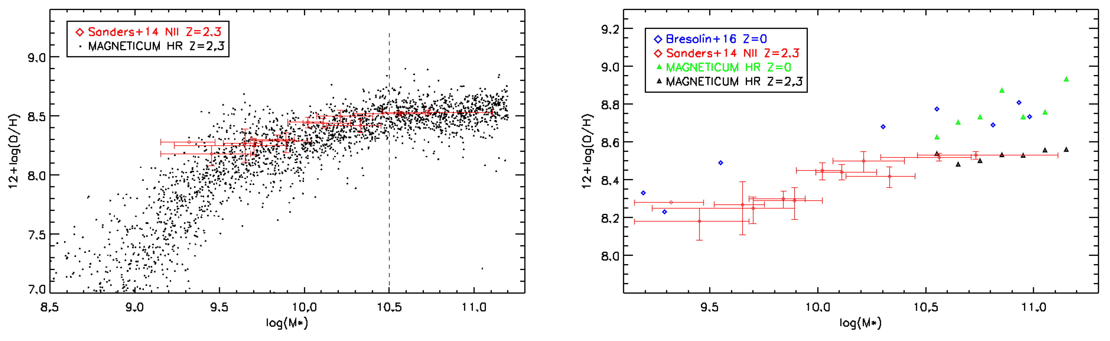
To estimate the gas-phase metallicity of galaxies, it is important to consider that observationally, the measurements are obtained only from star-forming regions. Therefore, it can be misleading to only calculate the mean metallicity of all gas particles inside a simulated galaxy. Thus, after selecting star-forming galaxies (see Teklu et al., 2017 [24]) we can either calculate their mean metallicity by averaging over all particles that are currently star-forming, or alternatively, calculate the mean metallicity of the newborn stars. We tested both methods and found that the latter gives slightly better results because of the fact that it is difficult to catch the metallicity of the gas phase in the moment of star formation within simulations, given the large timespan between the simulation outputs, while the young stellar population freezes the record of the metallicity of the gas from which it was formed. This leads to a MZR that is in good agreement with observations, as shown in the left panel of Figure 4, where we used the predicted oxygen abundances from our calculations to be consistent with observations (Sanders et al., 2015 [25] at $z=2.3$ and Bresolin et al., 2016 [26] at $z=0$). Interestingly, even the overall evolution of the MZR is well captured by the simulations and matches the observations, as demonstrated in the right panel of Figure 4. However, when calculating gas-phase metallicity gradients within the galaxies, the simulations predict a steeper profile than the observations. Given that the prediction of the mean metallicities is in good agreement with observations, this indicates that the simulations either still lack the resolution to properly describe the mixing of the enriched gas within galaxies, or that on these scales, the diffusion of metals might have to be modeled more explicitly. Nevertheless, we clearly showed that including detailed modeling of the stellar population, combined with current AGN feedback models, significantly improves the predicted ICM and IGM metallicities, and is needed to successfully reproduce various aspects of the observations.

4.3. Galaxies: Stellar Metallicities

In general, we assume that the mean metallicity of a stellar particle in the simulation represents the mean stellar metallicity of the stellar population represented by the stellar particle, neglecting any self-enrichment within stars. To be consistent with the observations, we based all calculations on the iron abundance, as predicted by the simulations. For this part of the study, we used a smaller cosmological volume with a higher resolution, as this allows for a classification of the galaxies due to their morphological type (see Teklu et al., 2015 [18] for more details on the classification and this particular simulation). This higher resolution also allows for a more detailed resolution of the metallicity gradients with the radius for individual galaxies.

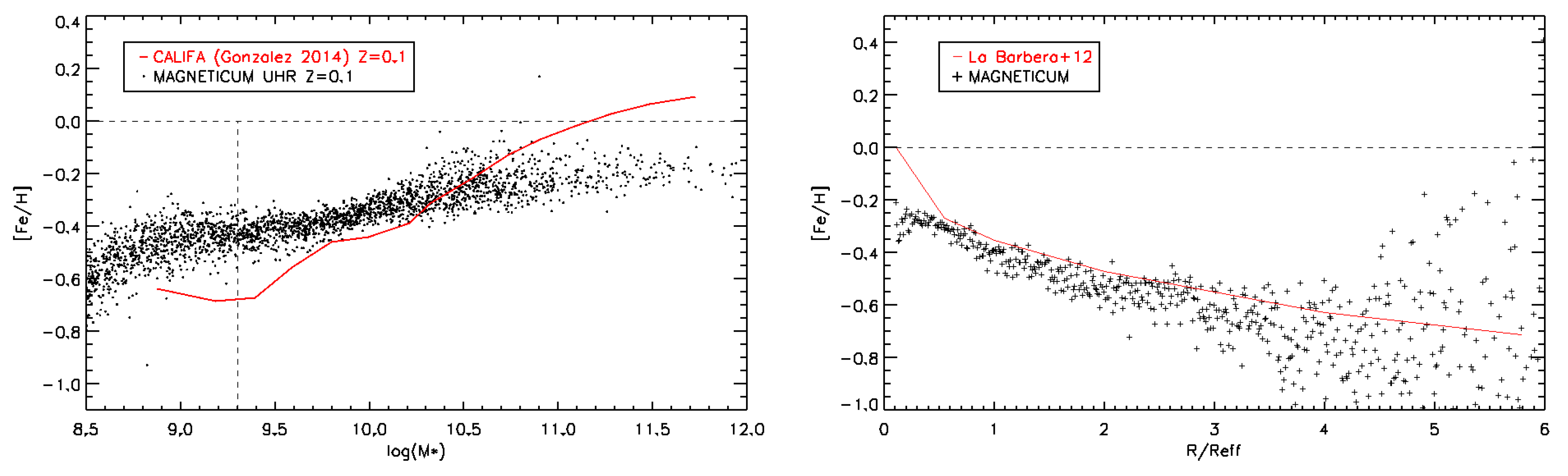
Although the obtained mean metallicities of our galaxies are close to observational results, the stellar MZR obtained from the simulations is somewhat shallower than that obtained from CALIFA observations by Gonzalez Delgado et al., 2014 [27], as shown in the left panel of Figure 5. This again indicates that the treatment of the mixing between accreted, more pristine material from outside the galaxy and the enriched gas within the galaxies is not fully captured yet. At this point, it is unclear whether this will be resolved by further enhancing the resolution of simulations, or whether explicit diffusion of metals has to be taken into account.

For a proper comparison of the radial metallicity gradients between simulations and observational data, it is necessary to calculate the effective radius $R_{\mathrm{eff}}$ for each galaxy. This is done by selecting all stellar particles within 10% of the virial radius and then inferring the according half-mass radius, which we associate to the effective radius $R_{\mathrm{eff}}$. This method has already been used to demonstrate that the Magneticum simulations successfully reproduce the mass–radius relation of galaxies for different morphological types (e.g., Remus et al., 2015 [28]) and at different redshifts (e.g., Remus et al., 2017 [19]).

Interestingly, the radial stellar metallicity gradients obtained from the simulations match the CALIFA observations very well, as shown in the right panel of Figure 5. We note also that the increasing spread towards a larger radius is an intrinsic, point-by-point spread within the individual galaxies, and that it agrees well with the behavior measured for individual galaxies by Pastorello et al., 2014 [29]. However, while the simulations successfully reproduce the observed iron abundances and radial gradients, they still produce a flat ratio of oxygen (or magnesium or silicium) over iron, in contrast to the observations, and here, the sub-grid model clearly needs to be advanced.

5. Discussion and Conclusions

Metals are measured in all phases of the baryonic universe, starting from the ICM in galaxy clusters down to gas and stars in individual galaxies. As the radial distribution of different types of metals encode a record of the star-formation process over the whole period of a galaxy’s evolution, comparing the chemical footprint, as seen in simulations, with observations reflects an excellent test on the reliability of the numerical sub-grid models included in modern state-of-the-art simulations of galaxy formation in a cosmological context in reproducing the complex processed involved in galaxy formation.

We demonstrated that the Magneticum simulations are able to reproduce a large variety of observational findings over a large range of halo masses, indicating that the star-formation and feedback processes included start to be highly realistic. At the galaxy-cluster scale, the simulations show an excellent agreement with both the absolute value and the cluster-by-cluster variation of the the iron abundance, when compared to X-ray observations, and they also broadly reproduce the chemical composition of the ICM. On galaxy scales, the tight mass–metallicity relations found for our simulated galaxies indicate that there are no strong secondary parameters (such as star-formation rates at a fixed redshift) driving the scatter in these relations. The remaining differences between the observed properties and the simulation results indicate, however, that the incorporation of physical processes such as diffusion and mixing have to be improved within the next generation of simulations to successfully reproduce the detailed distribution of metals on individually resolved galaxy scales.

References

- Dolag, K. Hydrodynamic Methods for Cosmological Simulations. In The Encyclopedia of Cosmology; Fazio, G.G., Ed.; World Scientific: Singapore, 2017; Volume 2. [Google Scholar]
- Matteucci, F. The Chemical Evolution of the Galaxy; Springer: Houten, Netherlands, 2003. [Google Scholar]
- Borgani, S.; Fabjan, D.; Tornatore, L.; Schindler, S.; Dolag, K.; Diaferio, A. The Chemical Enrichment of the ICM from Hydrodynamical Simulations. Space Sci. Rev. 2008, 134, 379–403. [Google Scholar] [CrossRef]
- Salpeter, E.E. The Luminosity Function and Stellar Evolution. Astrophys. J. 1955, 121, 161–167. [Google Scholar] [CrossRef]
- Chabrier, G. Galactic Stellar and Substellar Initial Mass Function. Publ. Astron. Soc. Pac. 2003, 115, 763–795. [Google Scholar] [CrossRef]
- Padovani, P.; Matteucci, F. Stellar Mass Loss in Elliptical Galaxies and the Fueling of Active Galactic Nuclei. Astrophys. J. 1993, 416, 26. [Google Scholar] [CrossRef]
- Maeder, A.; Meynet, G. Grids of evolutionary models from 0.85 to 120 solar masses—Observational tests and the mass limits. Astron. Astrophys. 1989, 210, 155–173. [Google Scholar]
- Chiappini, C.; Matteucci, F.; Gratton, R. The Chemical Evolution of the Galaxy: The Two-Infall Model. Astrophys. J. 1997, 477, 765–780. [Google Scholar] [CrossRef]
- Karakas, A.; Lattanzio, J.C. Stellar Models and Yields of Asymptotic Giant Branch Stars. Publ. Astron. Soc. Pac. 2007, 24, 103–117. [Google Scholar] [CrossRef]
- Nomoto, K.; Kobayashi, C.; Tominaga, N. Nucleosynthesis in Stars and the Chemical Enrichment of Galaxies. Ann. Rev. Astron. Astrophys. 2013, 51, 457–509. [Google Scholar] [CrossRef]
- Thielemann, F.K.; Argast, D.; Brachwitz, F.; Hix, W.R.; Höflich, P.; Liebendörfer, M.; Martinez-Pinedo, G.; Mezzacappa, A.; Nomoto, K.; Panov, I. Supernova Nucleosynthesis and Galactic Evolution. In From Twilight to Highlight: The Physics of Supernovae; Hillebrandt, W., Leibundgut, B., Eds.; Springer: Berlin, Germany, 2003; p. 331. [Google Scholar]
- Greggio, L.; Renzini, A. The binary model for type I supernovae—Theoretical rates. Astron. Astrophys. 1983, 118, 217–222. [Google Scholar]
- Greggio, L. The rates of type Ia supernovae. I. Analytical formulations. Astron. Astrophys. 2005, 441, 1055–1078. [Google Scholar] [CrossRef]
- Matteucci, F.; Gibson, B.K. Chemical abundances in clusters of galaxies. Astron. Astrophys. 1995, 304, 11. [Google Scholar]
- Matteucci, F.; Greggio, L. Relative roles of type I and II supernovae in the chemical enrichment of the interstellar gas. Astron. Astrophys. 1986, 154, 279–287. [Google Scholar]
- Bocquet, S.; Saro, A.; Dolag, K.; Mohr, J.J. Halo mass function: baryon impact, fitting formulae, and implications for cluster cosmology. Mon. Not. R. Astron. Soc. 2016, 456, 2361–2373. [Google Scholar] [CrossRef]
- Pollina, G.; Hamaus, N.; Dolag, K.; Weller, J.; Baldi, M.; Moscardini, L. On the linearity of tracer bias around voids. Mon. Not. R. Astron. Soc. 2017, 469, 787–799. [Google Scholar] [CrossRef]
- Teklu, A.F.; Remus, R.S.; Dolag, K.; Beck, A.M.; Burkert, A.; Schmidt, A.S.; Schulze, F.; Steinborn, L.K. Connecting Angular Momentum and Galactic Dynamics: The Complex Interplay between Spin, Mass, and Morphology. Astrophys. J. 2015, 812, 29. [Google Scholar] [CrossRef]
- Remus, R.S.; Dolag, K.; Naab, T.; Burkert, A.; Hirschmann, M.; Hoffmann, T.L.; Johansson, P.H. The co-evolution of total density profiles and central dark matter fractions in simulated early-type galaxies. Mon. Not. R. Astron. Soc. 2017, 464, 3742–3756. [Google Scholar] [CrossRef]
- Hirschmann, M.; Dolag, K.; Saro, A.; Bachmann, L.; Borgani, S.; Burkert, A. Cosmological simulations of black hole growth: AGN luminosities and downsizing. Mon. Not. R. Astron. Soc. 2014, 442, 2304–2324. [Google Scholar] [CrossRef]
- Biffi, V.; Planelles, S.; Borgani, S.; Fabjan, D.; Rasia, E.; Murante, G.; Tornatore, L.; Dolag, K.; Granato, G.L.; Gaspari, M.; et al. The history of chemical enrichment in the intracluster medium from cosmological simulations. Mon. Not. R. Astron. Soc. 2017, 468, 531–548. [Google Scholar] [CrossRef]
- Santini, P.; Maiolino, R.; Magnelli, B.; Lutz, D.; Lamastra, Z.; Li Causi, G.; Eales, S.; Andreani, P.; Berta, S.; Buat, V.; et al. The evolution of the dust and gas content in galaxies. Astron. Astrophys. 2014, 562, A30. [Google Scholar] [CrossRef] [Green Version]
- De Plaa, J.; Werner, N.; Bleeker, J.A.M.; Vink, J.; Kaastra, J.S.; Méndez, M. Constraining supernova models using the hot gas in clusters of galaxies. Astron. Astrophys. 2007, 465, 345–355. [Google Scholar] [CrossRef]
- Teklu, A.F.; Remus, R.S.; Dolag, K.; Burkert, A. The Morphology-Density-Relation: Impact on the Satellite Fraction. ArXiv, 2017; arXiv:1702.06546. [Google Scholar]
- Sanders, R.L.; Shapley, A.E.; Kriek, M.; Reddy, N.A.; Freeman, W.R.; Coil, A.L.; Siana, B.; Mobasher, B.; Shivaei, I.; Price, S.H.; et al. The MOSDEF Survey: Mass, Metallicity, and Star-formation Rate at z ∼ 2.3. Astrophys. J. 2015, 799, 138. [Google Scholar] [CrossRef]
- Bresolin, F.; Kudritzki, R.; Urbaneja, M.A.; Gieren, W.; Ho, I.; Pietrzyński, G. Young stars and ionized nebulae in M83: Comparing chemical abundances at high metallicity. Astrophys. J. 2016, 830, 64–85. [Google Scholar] [CrossRef]
- González Delgado, R.M.; Cid Fernandes, R.; Garcia-Benito, R.; Perez, E.; de Amorim, A.L.; Cortijo-Ferrero, C.; Lacerda, E.A.D.; Lopez Fernandez, R.; Sanchez, S.F.; Vale Asari, N.; et al. Insights on the Stellar Mass-Metallicity Relation from the CALIFA Survey. Astrophys. J. 2014, 791, L16. [Google Scholar] [CrossRef]
- Remus, R.S.; Dolag, K.; Bachmann, L.K.; Beck, A.M.; Burkert, A.; Hirschmann, M.; Teklu, A. Disk Galaxies in the Magneticum Pathfinder Simulations. In Galaxies in 3D across the Universe, Proceedings of the International Astronomical Union (IAU) Symposium, Vienna, Austria, 7–11 July 2014; Ziegler, B.L., Combes, F., Dannerbauer, H., Verdugo, M., Eds.; Cambridge University Press: Cambridge, UK, 2015; Volume 309, pp. 145–148. [Google Scholar]
- Pastorello, N.; Forbes, D.A.; Foster, C.; Brodie, J.P.; Usher, C.; Romanowsky, A.J.; Strader, J.; Arnold, J.A. The SLUGGS survey: exploring the metallicity gradients of nearby early-type galaxies to large radii. Mon. Not. R. Astron. Soc. 2014, 442, 1003–1039. [Google Scholar] [CrossRef]
- La Barbera, F.; Ferreras, I.; de Carvalho, R.R.; Bruzual, G.; Charlot, S.; Pasquali, A.; Merlin, E. SPIDER—VII. Revealing the stellar population content of massive early-type galaxies out to 8Re. Mon. Not. R. Astron. Soc. 2012, 426, 2300–2317. [Google Scholar] [CrossRef]
Figure 1.
Visualization of the large-scale distribution of the gas and stellar components within Box0 (see Bocquet et al., 2016 [16]) of the Magneticum simulation set at redshift . The inlays show a consecutive zoom onto the most massive galaxy cluster, where the individual galaxies become visible.
Figure 2.
Redshift evolution of the star-formation efficiency (SFE; coloured points with error bars) from Herschel observations presented by Santini et al., 2014 [22] overlayed with the predicted median values at different redshifts from star-forming galaxies in the Magneticum simulations (black triangles).
Figure 3.
Comparison between the observed inter-cluster medium (ICM) metallicity within (black symbols with error bars) and the metallicities of galaxy clusters from the Magneticum simulations (red diamonds) as a function of the ICM temperature. Different panels show the ratios for different metal types, as indicated in the panels. From top left to bottom right, the relative contribution of supernovae Type Ia (SNIa) is expected to increase, while the relative contribution of supernovae Type II (SNII) is expected to decrease. Observational data are taken from De Plaa et al., 2007 [23].
Figure 4.
Gas-phase metallicity from Magneticum galaxies in comparison to observational data by Sanders et al., 2015 [25] at redshift (red datapoints with error bars) and Bresolin et al., 2016 [26] at redshift (blue diamonds). Left panel: Each black point represents a galaxy from the simulation. Right panel: Median values for each mass bin at (black) and (green) are shown as triangles.
Figure 5.
Left panel: Stellar metallicity versus stellar mass obtained from the Magneticum galaxies (black dots), in comparison with observational data for galaxies independent of their morphology from Gonzalez Delgado et al., 2014 [27] at redshift . Right panel: Mean stellar radial metallicity gradient from 100 Magneticum galaxies in 100 radial bins normalized to the half-mass radius (black dots), compared to the observed profile from La Barbera et al., 2012 [30] (red line).