
Padé Approximant and Minimax Rational Approximation in Standard Cosmology


Dipartimento di Fisica, Università degli Studi di Torino, via P.Giuria 1, I-10125 Turin, Italy
Galaxies 2016, 4(1), 4; https://doi.org/10.3390/galaxies4010004
Submission received: 12 November 2015
/
Revised: 21 January 2016
/
Accepted: 21 January 2016
/
Published: 18 February 2016
Abstract
:The luminosity distance in the standard cosmology as given by ΛCDM and, consequently, the distance modulus for supernovae can be defined by the Padé approximant. A comparison with a known analytical solution shows that the Padé approximant for the luminosity distance has an error of at redshift . A similar procedure for the Taylor expansion of the luminosity distance gives an error of at redshift ; this means that for the luminosity distance, the Padé approximation is superior to the Taylor series. The availability of an analytical expression for the distance modulus allows applying the Levenberg–Marquardt method to derive the fundamental parameters from the available compilations for supernovae. A new luminosity function for galaxies derived from the truncated gamma probability density function models the observed luminosity function for galaxies when the observed range in absolute magnitude is modeled by the Padé approximant. A comparison of ΛCDM with other cosmologies is done adopting a statistical point of view.
Keywords:
cosmology; observational cosmology; distances; redshifts; radial velocities; spatial distribution of galaxies; magnitudes and colors; luminositiesPACS:
98.80.-k; 98.80.Es; 98.62.Py; 98.62.Qz1. Introduction
In order to obtain astronomical observables, such as the distance modulus and the absolute magnitude for supernovae (SN) of Type Ia in the standard cosmological approach, as given by the ΛCDM model, we need the evaluation of the luminosity distance, which is derived from the comoving distance. At the moment of writing, there is no analytical expression for the integral of the comoving distance in ΛCDM, and a numerical integration should be implemented. An analytical expression for the integral of the comoving distance in ΛCDM can be obtained by adopting the technique of the Padé approximant; see [1,2,3]. Once an approximate solution is obtained for the luminosity distance, we can evaluate the distance modulus and the absolute magnitude for SNs. Furthermore, the minimax rational approximation can provide a compact formula for the two above astronomical observables as functions of the redshift. From an observational point of view, the progressive increase in the number of supernova (SN) of Type Ia for which the distance modulus is available, 34 SNein the sample, which produced evidence for the accelerating universe (see [4]), 580 SNe in the Union 2.1 compilation (see [5]) and 740 SNe in the joint light-curve analysis (JLA) (see [6]), allows analyzing both the ΛCDM and other cosmologies from a statistical point of view. The statistical approach to cosmology is not new and has been recently adopted by [7,8]. In order to cover the previous arguments, Section 2 introduces the Padé approximant and determines the basic integral of the ΛCDM, which allows deriving the approximate luminosity distance. The approximate magnitude here derived is applied to parametrize a new luminosity function for galaxies at high redshift; see Section 3. The distance modulus in different cosmologies is reviewed, and the main statistical parameters connected with the distance modulus are derived; see Section 4.
2. The Standard Cosmology
This section introduces the Hubble distance, the dark energy density, the curvature, the matter density and the comoving distance (which is presented as the integral of the inverse of the Hubble function). In the absence of a general analytical formula for the comoving distance, we introduce the Padé approximation. As a consequence, we deduce an approximate solution for the transverse comoving distance, the luminosity distance and the distance modulus. The shift that the Padé approximation introduces in the relationship for the poles is discussed. The calibration of the Padé approximation for the distance modulus on two astronomical catalogs allows deducing the minimax polynomial approximation for the observed distance modulus for SNs of Type Ia.
2.1. The Padé Approximant
We use the same symbols as in [9], where the Hubble distance is defined as:
We then introduce the first parameter:
where G is the Newtonian gravitational constant and is the mass density at the present time. The second parameter is :
where Λ is the cosmological constant; see [10]. The two previous parameters are connected with the curvature by:
The comoving distance, , is:
where is the `Hubble function’:
The above integral does not have an analytical formula, except for the case of , but the Padé approximant (see Appendix B) gives an approximate evaluation, and the indefinite integral is (B3), where the coefficients and can be found in Appendix A. The approximate definite integral for (5) is therefore:
The transverse comoving distance is:
and the approximate transverse comoving distance computed with the Padé approximant is:
An analytic expression for can be obtained when: :
This expression is useful for calibrating the numerical codes, which evaluate when .
The luminosity distance is:
which in the case of becomes:
and the distance modulus when is:
The Padé approximant luminosity distance when is:
and the Padé approximant distance modulus, , in its compact version, is:
and, as a consequence, the Padé approximant absolute magnitude, , is:
The expanded version of the Padé approximant distance modulus is:
with:
The above procedure can also be applied when the argument of the integral (5) is expanded about z = 0 in a Taylor series of order six. The resulting luminosity distance, , is:
where:
2.2. The Presence of Poles
The equation which models the poles is:
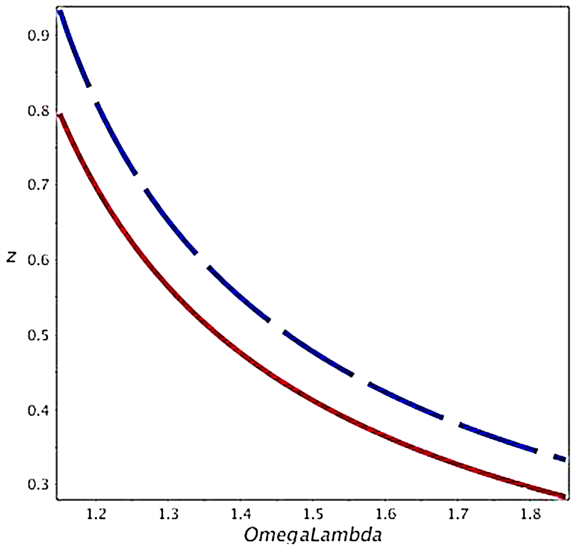
The exact solution of the above equation is shown in Figure 4, together with the Padé approximated solution . Is therefore possible to conclude that the Padé approximation shifts the locations of the poles by ; this shift expressed as a percentage error is in the considered interval .
2.3. An Astrophysical Application
We now have a Padé approximant expression for the distance modulus as a function of of , and . We now perform an astronomical test on the 580 SNe in the Union 2.1 compilation (see [5]) and on the 740 SNe in the joint light-curve analysis (JLA). The JLA compilation is available at the Strasbourg Astronomical Data Center (CDS) and consists of SNe (Type I-a) for which we have a heliocentric redshift, z, apparent magnitude in the B band, error in , , parameter , error in , , parameter C, error in the parameter C, and . The observed distance modulus is defined by Equation (4) in [6]:
The adopted parameters are , and:
see Line 1 in Table 10 of [6]. The uncertainty in the observed distance modulus, , is found by implementing the error propagation equation (often called the law of errors of Gauss) when the covariant terms are neglected; see Equation (3.14) in [11],
The three astronomical parameters in question, , and , can be derived trough the Levenberg–Marquardt method (subroutine MRQMINin [12]) once an analytical expression for the derivatives of the distance modulus with respect to the unknown parameters is provided. As a practical example, the derivative of the distance modulus, , with respect to is:
This numerical procedure minimizes the merit function evaluated as:
where , is the observed distance modulus evaluated at , is the error in the observed distance modulus evaluated at and is the theoretical distance modulus evaluated at ; see Formula (15.5.5) in [12]. A reduced merit function is evaluated by:
where is the number of degrees of freedom, n is the number of SNe and k is the number of parameters. Another useful statistical parameter is the associated Q-value, which has to be understood as the maximum probability of obtaining a better fitting; see Formula (15.2.12) in [12]:
where GAMMQ is a subroutine for the incomplete gamma function. The Akaike information criterion (AIC) (see [13]) is defined by:
where L is the likelihood function. We assume a Gaussian distribution for the errors, and the likelihood function can be derived from the statistic , where has been computed by Equation (26); see [14,15]. Now, the AIC becomes:
Table 1 reports the three astronomical parameters for the two catalogs of SNs, and Figure 5 and Figure 6 display the best fits.
In order to see how varies around the minimum found by the Levenberg–Marquardt method, Figure 7 presents a 2D color map for the values of when and are allowed to vary around the numerical values, which fix the minimum.
The Padé approximant distance modulus has a simple expression when the minimax rational approximation is used, as an example ; see Appendix C for the meaning of p and q. In the case of the Union 2.1 compilation, the approximation of Formula (17) with the parameters of Table 1 over the range in gives the following minimax equation:
the maximum error being 0.0024. The maximum error of the polynomial approximation as a function of p and q is shown in Table 2.
In the case of the JLA compilation, the minimax equation is:
the maximum error being 0.003.
3. Application at High Redshift
This section introduces a new luminosity function (LF) for galaxies, which has a lower and an upper bound. The presence of a lower bound for the luminosity of galaxies allows one to model the evolution of the LF as a function of the redshift.
3.1. The Schechter Luminosity Function
The Schechter LF, after [16], is the standard LF for galaxies:
Here, α sets the shape, is the characteristic luminosity and is the normalization. The distribution in absolute magnitude is:
where is the characteristic magnitude.
3.2. The Gamma Luminosity Function
The gamma LF is:
where is the total number of galaxies per unit Mpc,
is the gamma function, is the scale and is the shape; see Formula (17.23) in [17]. Its expected value is:
The change of parameter allows obtaining the same scaling as for the Schechter LF (34).
3.3. The Truncated Gamma Luminosity Function
We assume that the luminosity L takes values in the interval where the indices l and u mean lower and upper; the truncated gamma LF is:
where is the total number of galaxies per unit Mpc, and the constant k is:
where:
is the upper incomplete gamma function; see [18,19]. Its expected value is:
More details on the truncated gamma PDF can be found in [20,21]. The four luminosities and are connected to the absolute magnitude M, , and through the following relationship:
where the indices u and l are inverted in the transformation from luminosity to absolute magnitude, and is the absolute magnitude of the Sun in the considered band. The gamma truncated LF in magnitude is:
where
The first test on the reliability of the truncated gamma LF was performed on the data of the Sloan Digital Sky Survey (SDSS) (see [22]) in the band . The number of variables can be reduced to two once and are identified with the maximum and minimum absolute magnitude of the considered sample. The LFs considered here are displayed in Figure 8. A second test is represented by the behavior of the LF at high z. We expect a progressive decrease of the low luminosity galaxies (high magnitude) when z is increasing. A formula that models the previous statement can be obtained by Equation (16), which models the absolute magnitude, M, as a function of the redshift, inserting as the apparent magnitude, m, the limiting magnitude of the considered catalog. We now outline how to build an observed LF for a galaxy in a consistent way; the selected catalog is zCOSMOS, which is made up of 9697 galaxies up to 4; see [23]. The observed LF for zCOSMOS can be built by employing the following algorithm.
- (1)
- The minimax approximation for the luminosity distance in the case of the JLA compilation parameters (see Equation (33b)) allows fixing the distance, in the following r, once z is given.
- (2)
- A value for the redshift is fixed, z, as well as the thickness of the layer, .
- (3)
- All of the galaxies comprised between z and are selected.
- (4)
- The absolute magnitude is computed from Equation (16).
- (5)
- The distribution in magnitude is organized in frequencies versus absolute magnitude.
- (6)
- The frequencies are divided by the volume, which is , where r is the considered radius, is the thickness of the radius and Ω is the solid angle of ZCOSMOS.
- (7)
- The error in the observed LF is obtained as the square root of the frequencies divided by the volume.
4. Different Cosmologies
Here, we analyze the distance modulus for SNe in other cosmologies in the framework of general relativity (GR), an expanding flat universe, special relativity (SR) and a Euclidean static universe.
4.1. Simple GR Cosmology
In the framework of GR, the received flux, f, is:
where is the luminosity distance, which depends on the cosmological model adopted; see Equation (7.21) in [24] or Equation (5.235) in [25].
The distance modulus in the simple GR cosmology is:
see Equation (7.52) in [24]. The number of free parameters in the simple GR cosmology is two: and .
4.2. Flat Expanding Universe
This model is based on the standard definition of luminosity in the flat expanding universe. The luminosity distance, , is:
and the distance modulus is:
see Formulae (13) and (14) in [26]. The number of free parameters in the flat expanding model. is one: .
4.3. Einstein–De Sitter Universe in SR
In the Einstein–De Sitter model, which is developed in SR, the luminosity distance, after [27,28], is:
and the distance modulus for the Einstein–De Sitter model is:
The number of free parameters in the Einstein–De Sitter model is one: .
4.4. Milne Universe in SR
In the Milne model, which is developed in the framework of SR, the luminosity distance, after [29,30,31], is:
and the distance modulus for the Milne model is:
The number of free parameters in the Milne model is one: .
4.5. Plasma Cosmology
In a Euclidean static framework, among many possible absorption mechanisms, we selected a photo-absorption process between the photon and the electron in the IGM. This relativistic process produces a nonlinear dependence between redshift and distance:
see Equation (4) in [32]. The previous equation is identical to our Equation (59). The Hubble constant in this first plasma model is:
where <> is expressed in cgsunits. The second mechanism is a plasma effect, which produces the following relationship:
see Equation (50) in [33]. Furthermore, this second mechanism produces the same nonlinear d-z dependence as our Equation (59). In the presence of plasma absorption, the observed flux is:
where the factor is due to Galactic and host galactic extinctions, is reduction to the plasma in the IGM and is the reduction due to Compton scattering; see the formula before Equation (51) in [33]. The resulting distance modulus in the plasma mechanism is:
see Equation (7) in [34]. The number of free parameters in the plasma cosmology is one: when .
4.6. Modified Tired Light
In a Euclidean static framework, the modified tired light (MTL) has been introduced in Section 2.2 in [35]. The distance in MTL is:
The distance modulus in the modified tired light (MTL) is:
Here, β is a parameter comprised between one and three, which allows one to match theory with observations. The number of free parameters in MTL is two: and β.
4.7. Results for Different Cosmologies
5. Conclusions
5.1. Padé approximant
It is generally thought that in the case of the luminosity distance, the Padé approximant is more accurate than the Taylor expansion. As an example, at , which is the maximum value of the redshift here considered, the percentage error of the luminosity distance is in the case of the Padé approximation. In the case of of the Taylor expansion, for the luminosity distance is reached , which means a more limited range of convergence than for the Padé approximation. Once a precise approximation for the luminosity distance was obtained (see Equation (11)), we derived an approximate expression for the distance modulus (see Equation (17)) and the absolute magnitude (see Equation (16)).
5.2. Astrophysical Applications
The availability of the observed distance modulus for a great number of SNs of Type Ia allows deducing , and for two catalogs; see Table 1. In order to derive the above parameters, the Levenberg–Marquardt method was implemented, and therefore, the first derivative of the distance modulus (see Equation (17)) with respect to three parameters is provided. The value of is a matter of research rather than a well-defined constant. As an example, a recent evaluation with a sample of Cepheids gives ; see [36]. Once the above value is considered the `true’ value, we have found, adopting the Padé approximant, , which means a percentage error , for the Union 2.1 compilation, and , which means a percentage error , for the JLA compilation; see Table 1.
5.3. Evolutionary Effects
The evolution of the LF for galaxies as a function of the redshift is here modeled by an upper and lower truncated gamma PDF. This choice allows modeling the lower bound in luminosity (the higher bound in absolute magnitude) according to the evolution of the absolute magnitude; see Equation (16). According to the LF here considered (see Equation (44)), the evolution with z of the LF is simply connected to the evolution of the higher bound in absolute magnitude; see Figure 9, Figure 10 and Figure 11. Is not necessary to modify the shape parameters of the LF, which are c and , but only to calculate the normalization at different values of the redshift.
5.4. Statistical Tests for Union 2.1
In the case of the Union 2.1 compilation, the best results for are obtained by the ΛCDM cosmology (GR), , against of the MTL cosmology (Euclidean), but the situation is inverted when the AIC is considered: the AIC is 571.9 for the MTL cosmology and 568.7 for the ΛCDM cosmology (GR); see Table 1 and Table 5.
The simple model (GR), the Einstein–De Sitter model (SR), the Milne model (SR) and the plasma model (Euclidean) are rejected because the reduced merit function is smaller than one; see Table 5. The best performing one-parameter model is that of Milne, , followed by the flat expanding model, ; see Table 5.
5.5. Statistical Tests for JLA
In the case of the JLA compilation, the best results for are obtained by the MTL cosmology (Euclidean), , against for the ΛCDM cosmology (GR); see Table 1 and Table 6. The simple model (GR), the Einstein–De Sitter model (SR) and the plasma model (Euclidean) are rejected because the reduced merit function is smaller than one; see Table 6. In the case of the JLA, the test on the Milne model is positive because is smaller than one. The best performing one-parameter model is that of Milne, , followed by the flat expanding model, ; see Table 6.
5.6. Different Approaches
Table 7 reports six items connected to the use of the Padé approximant in Cosmology: the letters Y/N indicate if the item is treated or not, and the columns identifies the paper in question; LF means the luminosity function for galaxies.
Conflicts of Interest
The authors declare no conflict of interest.
Appendix
A. The Padé Approximant
The coefficients and are found through Wynn’s cross rule (see [38,39]), and our choice is and . The choice of p and q is a compromise between precision, high values for p and q and the simplicity of the expressions to manage low values for p and q; Appendix B gives three different approximations for the indefinite integral for three different combinations in p and q. In the case in which , we can divide both the numerator and denominator by , reducing by one the number of parameters; see as an example [40].
B. The Integrals as Functions of p and q
In the case ,
In the case ,
In the case ,
C. Minimax Approximation
Let be a real function defined in the interval . The best rational approximation of degree evaluates the coefficients of the ratio of two polynomials of degree k and l, respectively, which minimizes the maximum difference of:
on the interval . The quality of the fit is given by the maximum error over the considered range. The coefficients are evaluated through the Remez algorithm; see [41,42]. As an example, the minimax of degree (2,2) of:
is:
and the maximum error is . As an example, the minimax rational function approximation is applied to the evaluation of the complete elliptic integral of the first and second kind; see [43].
References
- Adachi, M.; Kasai, M. An Analytical Approximation of the Luminosity Distance in Flat Cosmologies with a Cosmological Constant. Prog. Theor. Phys. 2012, 127, 145–152. [Google Scholar] [CrossRef]
- Aviles, A.; Bravetti, A.; Capozziello, S.; Luongo, O. Precision cosmology with Padé rational approximations: Theoretical predictions versus observational limits. Phys. Rev. D 2014, 90, 043531. [Google Scholar] [CrossRef]
- Wei, H.; Yan, X.P.; Zhou, Y.N. Cosmological applications of Pade approximant. J. Cosmol. Astropart. Phys. 2014, 1, 45. [Google Scholar] [CrossRef]
- Riess, A.G.; Filippenko, A.V.; Challis, P.; Clocchiatti, A. Observational Evidence from Supernovae for an Accelerating Universe and a Cosmological Constant. Astron. J. 1998, 116, 1009–1038. [Google Scholar] [CrossRef]
- Suzuki, N.; Rubin, D.; Lidman, C.; Aldering, G.; Amanullah, R.; Barbary, K.; Barrientos, L.F. The Hubble Space Telescope Cluster Supernova Survey. V. Improving the Dark-energy Constraints above z greater than 1 and Building an Early-type-hosted Supernova Sample. Astrophys. J. 2012, 746, 85. [Google Scholar] [CrossRef]
- Betoule, M.; Kessler, R.; Guy, J.; Mosher, J. Improved cosmological constraints from a joint analysis of the SDSS-II and SNLS supernova samples. Cosmol. Nongalactic Astrophys. 2014, 568, A22. [Google Scholar] [CrossRef] [Green Version]
- Montiel, A.; Lazkoz, R.; Sendra, I.; Escamilla-Rivera, C.; Salzano, V. Nonparametric reconstruction of the cosmic expansion with local regression smoothing and simulation extrapolation. Phys. Rev. D 2014, 89, 043007. [Google Scholar] [CrossRef]
- Yahya, S.; Seikel, M.; Clarkson, C.; Maartens, R.; Smith, M. Null tests of the cosmological constant using supernovae. Phys. Rev. D 2014, 89, 023503. [Google Scholar] [CrossRef]
- Hogg, D.W. Distance measures in cosmology. 1999. [Google Scholar]
- Peebles, P.J.E. Principles of Physical Cosmology; Princeton University Press: Princeton, NJ, USA, 1993. [Google Scholar]
- Bevington, P.R.; Robinson, D.K. Data Reduction and Error Analysis for the Physical Sciences; McGraw-Hill: New York, NY, USA, 2003. [Google Scholar]
- Press, W.H.; Teukolsky, S.A.; Vetterling, W.T.; Flannery, B.P. Numerical Recipes in FORTRAN. The Art of Scientific Computing; Cambridge University Press: Cambridge, UK, 1992. [Google Scholar]
- Akaike, H. A new look at the statistical model identification. IEEE Trans. Automatic Control 1974, 19, 716–723. [Google Scholar] [CrossRef]
- Liddle, A.R. How many cosmological parameters? Mon. Not. R. Astron. Soc. 2004, 351, L49–L53. [Google Scholar] [CrossRef]
- Godlowski, W.; Szydowski, M. Constraints on Dark Energy Models from Supernovae. In 1604–2004: Supernovae as Cosmological Lighthouses; Turatto, M., Benetti, S., Zampieri, L., Shea, W., Eds.; Astronomical Society of the Pacific: Orem, UT, USA, 2005; Volume 342, pp. 508–516. [Google Scholar]
- Schechter, P. An analytic expression for the luminosity function for galaxies. Astrophys. J. 1976, 203, 297–306. [Google Scholar] [CrossRef]
- Johnson, N.L.; Kotz, S.; Balakrishnan, N. Continuous Univariate Distributions, 2nd ed.; Wiley: New York, NY, USA, 1994; Volume 1. [Google Scholar]
- Abramowitz, M.; Stegun, I.A. Handbook of Mathematical Functions with Formulas, Graphs, and Mathematical Tables; Dover: New York, NY, USA, 1965. [Google Scholar]
- Olver, F.W.J.; Lozier, D.W.; Boisvert, R.F.; Clark, C.W. (Eds.) NIST Handbook of Mathematical Functions; Cambridge University Press: Cambridge, UK, 2010.
- Zaninetti, L. A right and left truncated gamma distribution with application to the stars. Adv. Stud. Theor. Phys. 2013, 23, 1139–1147. [Google Scholar]
- Okasha, M.K.; Alqanoo, I.M. Inference on The Doubly Truncated Gamma Distribution For Lifetime Data. Int. J. Math. Stat. Invent. 2014, 2, 1–17. [Google Scholar]
- Blanton, M.R.; Hogg, D.W.; Bahcall, N.A.; Brinkmann, J.; Britton, M. The Galaxy Luminosity Function and Luminosity Density at Redshift z = 0.1. Astrophys. J. 2003, 592, 819–838. [Google Scholar] [CrossRef]
- Lilly, S.J.; Le Brun, V.; Maier, C.; Mainieri, V. The zCOSMOS 10k-Bright Spectroscopic Sample. Astrophys. J. Suppl. 2009, 184, 218–229. [Google Scholar] [CrossRef]
- Ryden, B. Introduction to Cosmology; Addison Wesley: San Francisco, CA, USA, 2003. [Google Scholar]
- Lang, K. Astrophysical Formulae: Space, Time, Matter and Cosmology; Astronomy and Astrophysics Library, Springer: Berlin, Germany, 2013. [Google Scholar]
- Heymann, Y. On the Luminosity Distance and the Hubble Constant. Prog. Phys. 2013, 3, 5–6. [Google Scholar]
- Einstein, A.; de Sitter, W. On the Relation between the Expansion and the Mean Density of the Universe. Proc. Natl. Acad. Sci. USA 1932, 18, 213–214. [Google Scholar] [CrossRef] [PubMed]
- Krisciunas, K. Look-Back Time the Age of the Universe and the Case for a Positive Cosmological Constant. J. Roy. Astron. Soc. Can. 1993, 87, 223. [Google Scholar]
- Milne, E.A. World-Structure and the Expansion of the Universe. Zeitschrift fur Astrophysik 1933, 6, 1. [Google Scholar] [CrossRef]
- Chodorowski, M.J. Cosmology Under Milne’s Shadow. Publ. Astron. Soc. Austral. 2005, 22, 287–291. [Google Scholar] [CrossRef]
- Adamek, J.; Di Dio, E.; Durrer, R.; Kunz, M. Distance-redshift relation in plane symmetric universes. Phys. Rev. D 2014, 89, 063543. [Google Scholar] [CrossRef]
- Ashmore, L. Recoil Between Photons and Electrons Leading to the Hubble Constant and CMB. Galilean Electrodyn. 2006, 17, 53. [Google Scholar]
- Brynjolfsson, A. Redshift of photons penetrating a hot plasma. 2004. [Google Scholar]
- Brynjolfsson, A. Magnitude-Redshift Relation for SNe Ia, Time Dilation, and Plasma Redshift. 2006. [Google Scholar]
- Zaninetti, L. On the Number of Galaxies at High Redshift. Galaxies 2015, 3, 129–155. [Google Scholar] [CrossRef]
- Riess, A.G.; Macri, L.; Casertano, S.; Lampeitl, H.; Ferguson, H.C.; Filippenko, A.V.; Jha, S.W.; Li, W.; Chornock, R. A 3% Solution: Determination of the Hubble Constant with the Hubble Space Telescope and Wide Field Camera 3. Astrophys. J. 2011, 730, 119. [Google Scholar] [CrossRef]
- Padé, H. Sur la représentation approchée d’une fonction par des fractions rationnelles. Ann. Sci. Ecole Norm. Sup. 1892, 9, 193. [Google Scholar]
- Baker, G. Essentials of Padé Approximants; Academic Press: New York, NY, USA, 1975. [Google Scholar]
- Baker, G.A.; Graves-Morris, P.R. Padé approximants; Cambridge University Press: Cambridge, UK, 1996. [Google Scholar]
- Yamada, H.S.; Ikeda, K.S. A Numerical Test of Pade Approximation for Some Functions with singularity. Int. J. Comput. Math. 2014, 2014. [Google Scholar] [CrossRef]
- Remez, E. Sur la détermination des polynômes d´approximation de degré donnée. Comm. Soc. Math. Kharkov 1934, 10, 41–63. [Google Scholar]
- Remez, E. General Computation Methods of Chebyshev Approximation. The Problems with Linear Real Parameters; Publishing House of the Academy of Science of the Ukrainian SSR: Kiev, Ukraine, 1957. [Google Scholar]
- Fukushima, T. Precise and fast computation of the general complete elliptic integral of the second kind. Math. Comput. 2011, 80, 1725–1743. [Google Scholar] [CrossRef]
Figure 1.
Percentage error, δ, relative to the Taylor approximated luminosity distance (see Equation (18)) when and .
Figure 1.
Percentage error, δ, relative to the Taylor approximated luminosity distance (see Equation (18)) when and .
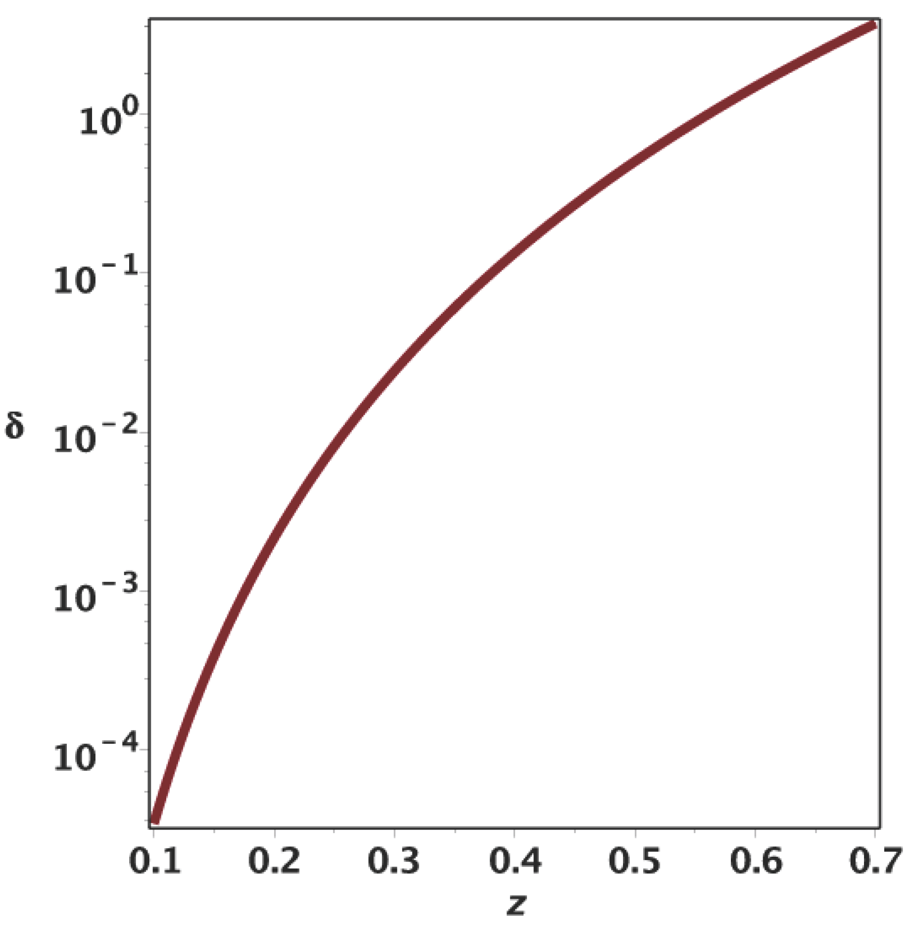
Figure 2.
Percentage error, δ, relative to the Padè approximated luminosity distance (see Equation (14)) when and .
Figure 2.
Percentage error, δ, relative to the Padè approximated luminosity distance (see Equation (14)) when and .
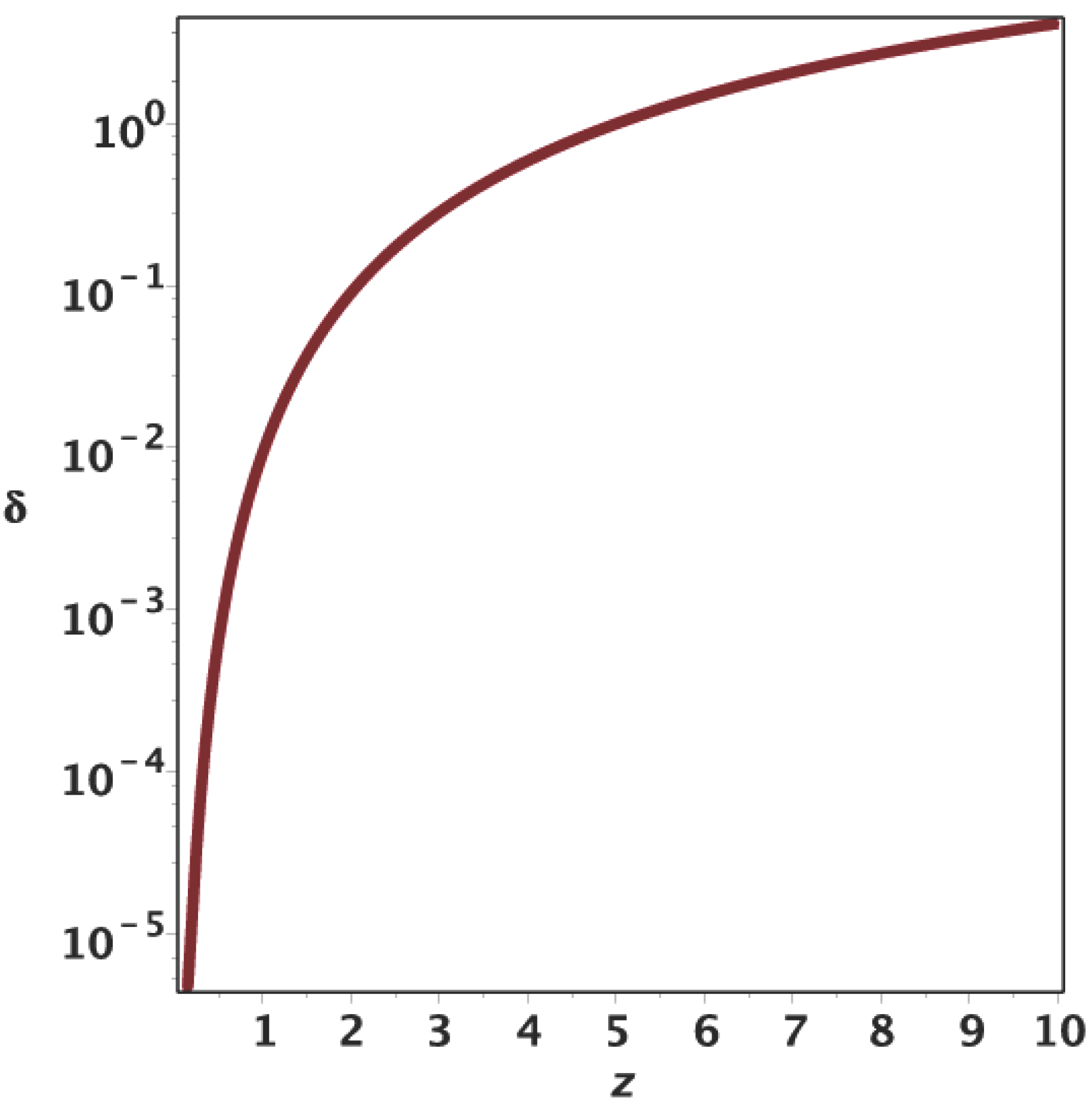
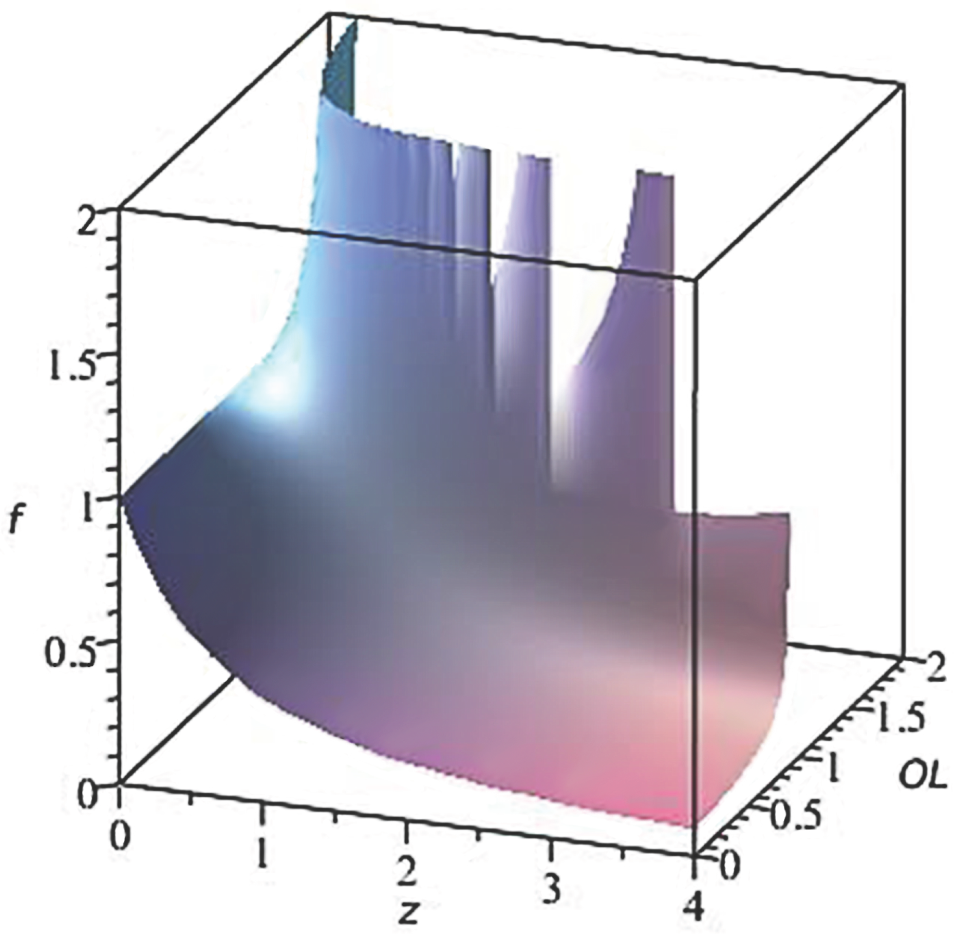
Figure 3.
Behavior of as a function of z and in the neighborhoods of the poles when .

Figure 4.
The exact solution for the zero in E(z), full red line, and Padé approximated solution, dashed blue line, when .
Figure 4.
The exact solution for the zero in E(z), full red line, and Padé approximated solution, dashed blue line, when .

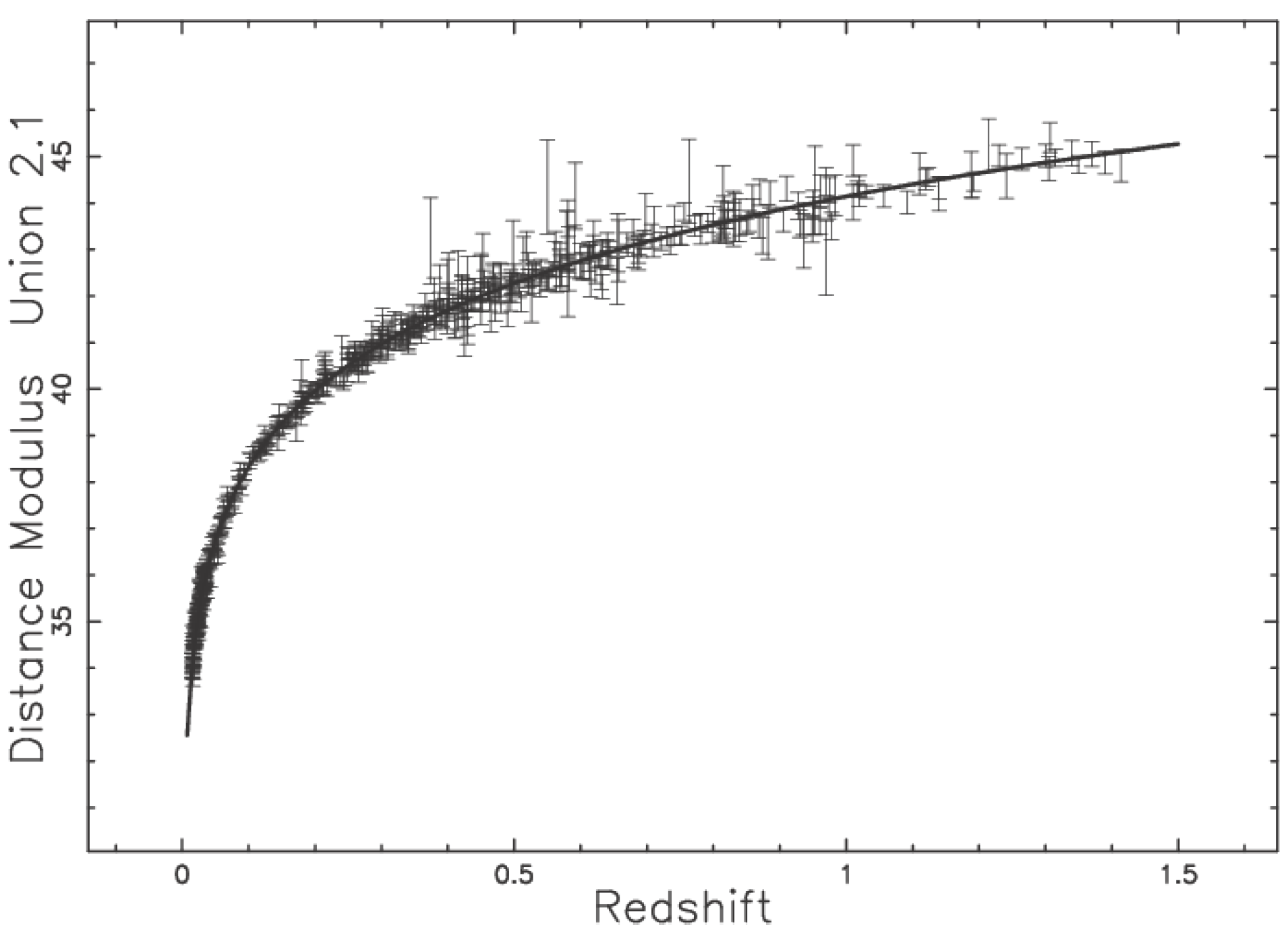
Figure 5.
Hubble diagram for the Union 2.1 compilation. The solid line represents the best fit for the approximate distance modulus as represented by Equation (17); parameters as in Table 1.

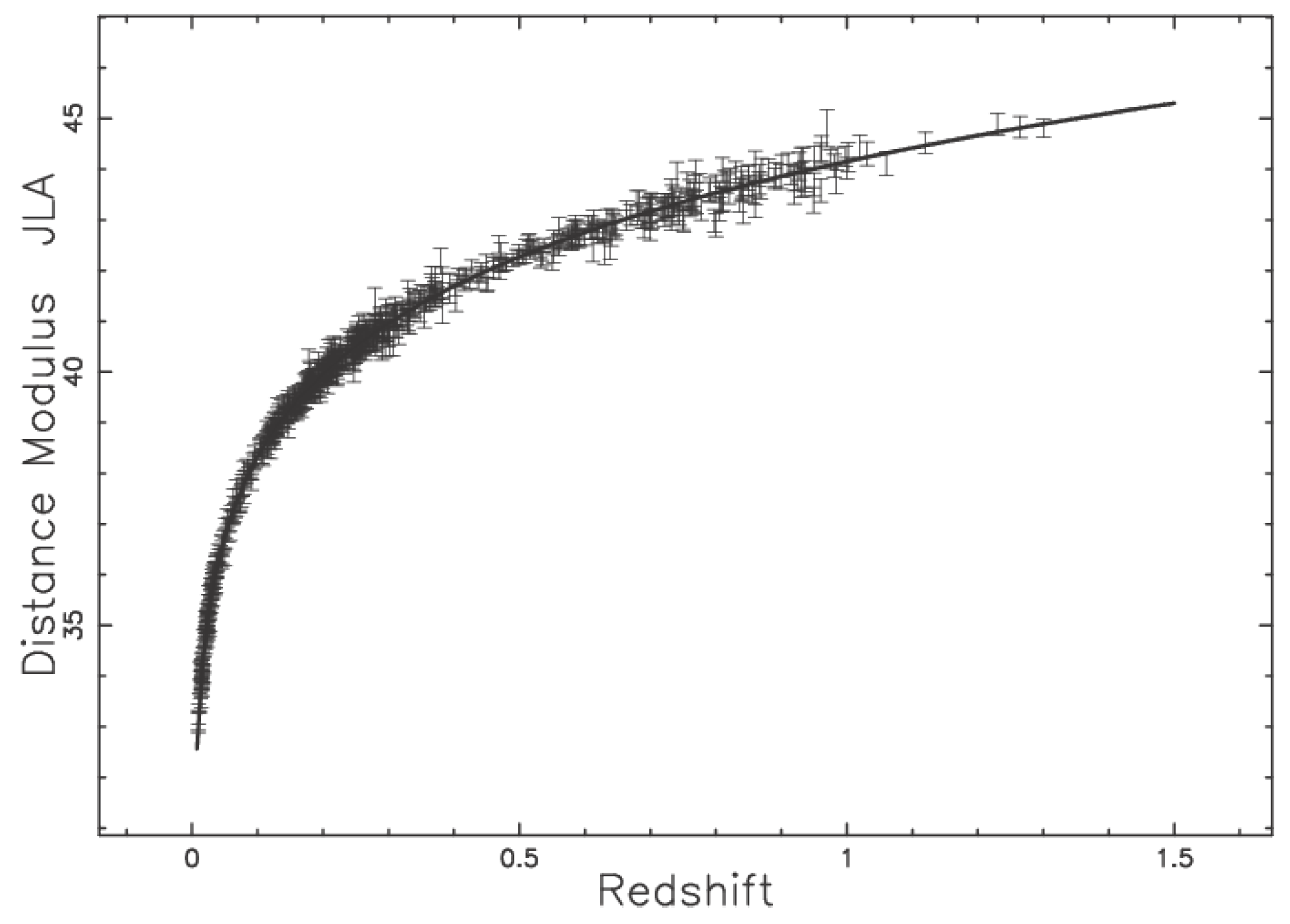
Figure 6.
Hubble diagram for the JLA compilation. The solid line represents the best fit for the approximate distance modulus as given by Equation (17); parameters as in Table 1.

Figure 7.
Color contour plot for of the Hubble diagram for the Union 2.1 compilation when and are variables and .
Figure 7.
Color contour plot for of the Hubble diagram for the Union 2.1 compilation when and are variables and .
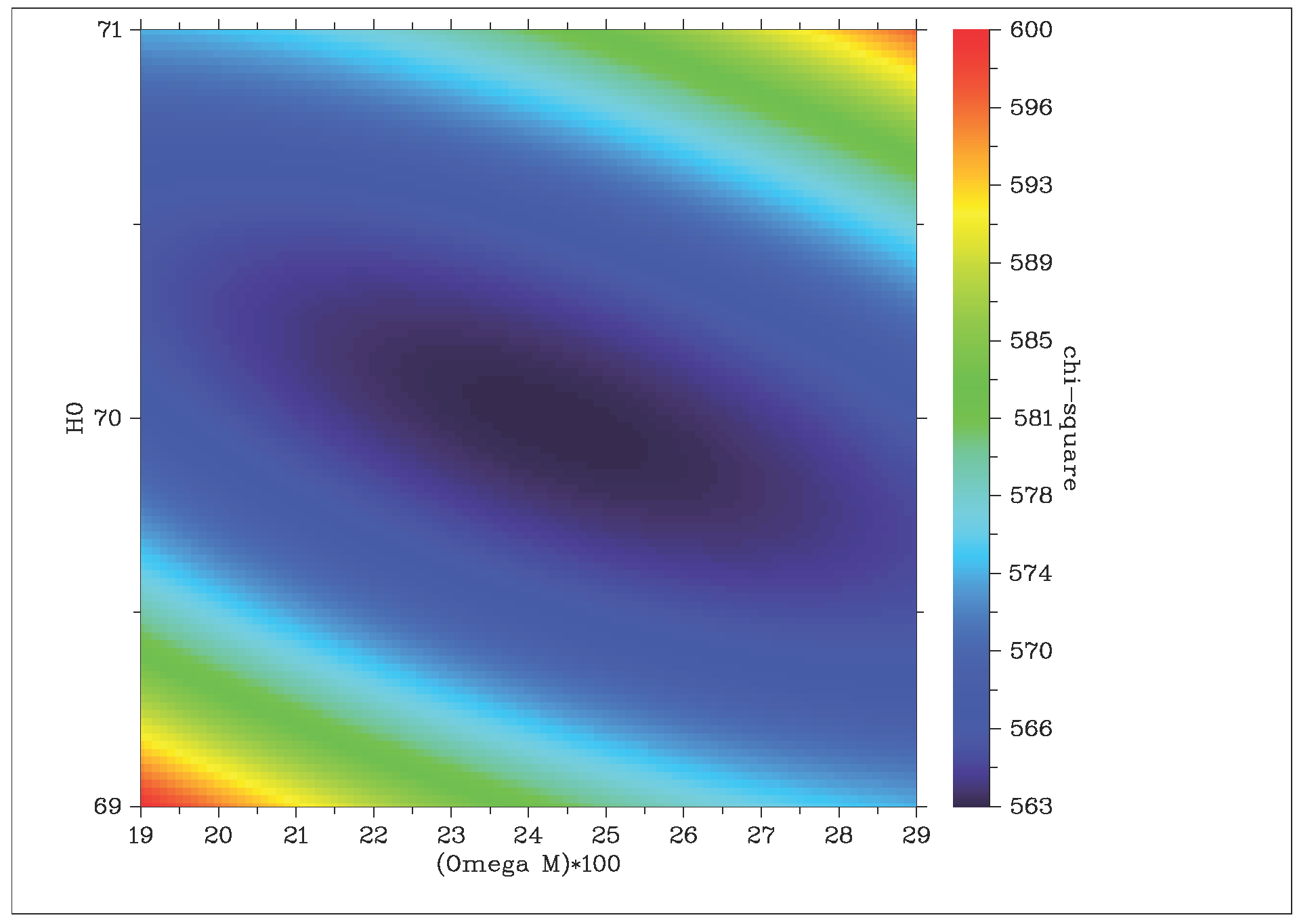
Figure 8.
The luminosity function data of the Sloan Digital Sky Survey (SDSS) () are represented with error bars. The continuous line fit represents our truncated gamma luminosity function (LF) (44) with parameters = −23.73, = −17.48, = −21.1, and . The dotted line represents the Schechter LF with parameters and .

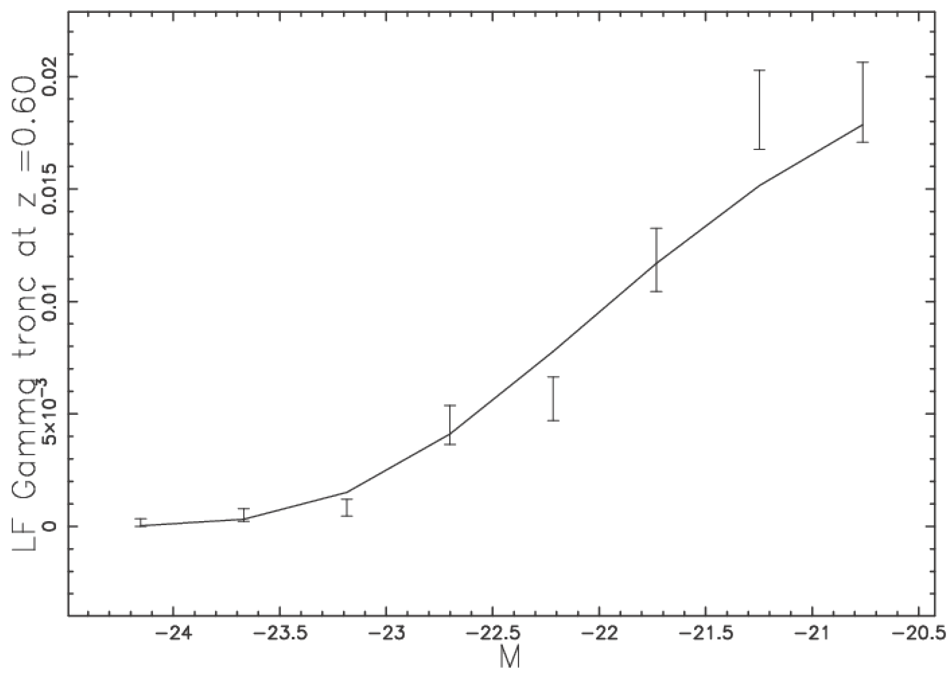
Figure 9.
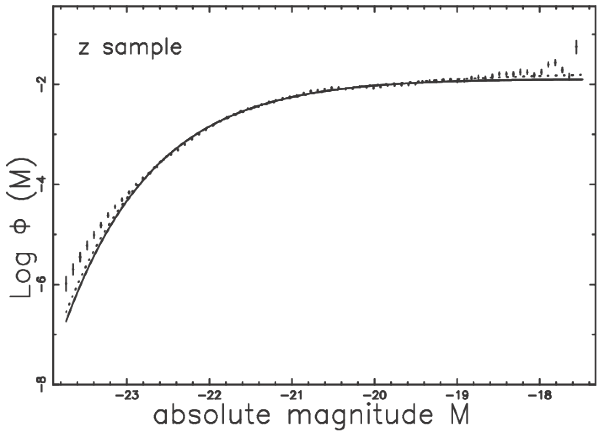
The luminosity function data of zCOSMOS are represented with error bars. The continuous line fit represents our gamma truncated LF (44); the chosen redshift is and = 0.05. The parameters independent of the redshift are given in Table 3, and the upper magnitude-zrelationship is given in Table 4.
Figure 9.
The luminosity function data of zCOSMOS are represented with error bars. The continuous line fit represents our gamma truncated LF (44); the chosen redshift is and = 0.05. The parameters independent of the redshift are given in Table 3, and the upper magnitude-zrelationship is given in Table 4.
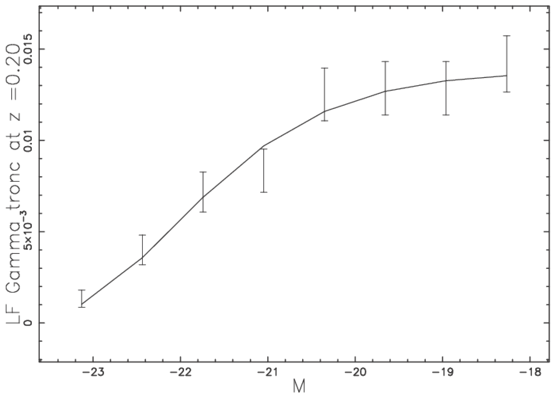
Figure 10.
The luminosity function data of zCOSMOSare represented with error bars. The continuous line fit represents our gamma truncated LF (44); the chosen redshift is and = 0.05. Parameters in Table 3 and Table 4.

Figure 11.
The luminosity function data of zCOSMOSare represented with error bars. The continuous line fit represents our gamma truncated LF (44); the chosen redshift is and = 0.05. Parameters in Table 3 and Table 4.

Table 1.
Numerical values of , , Q, and the AIC of the Hubble diagram for two compilations; k stands for the number of parameters. SN, supernoval; JLA, joint light-curve analysis.
| Compilation | SNs | k | Parameters | Q | AIC | ||
|---|---|---|---|---|---|---|---|
| Union 2.1 | 577 | 3 | = 69.81; ; | 562.699 | 0.975 | 0.657 | 568.699 |
| JLA | 740 | 3 | = 69.398; ; | 625.733 | 0.849 | 0.998 | 631.733 |
Table 2.
The maximum error in the minimax rational approximation for the distance modulus in the case of the Union 2.1 compilation.
| p | q | Maximum Error |
|---|---|---|
| 1 | 1 | 0.2872 |
| 2 | 2 | 0.0197 |
| 3 | 2 | 0.0024 |
| 3 | 3 | 0.0006 |
| Ml | M* | c |
|---|---|---|
| −23.47 | −22.7 | 0.01 |
| z | Ψ* | Mu |
|---|---|---|
| 0.2 | 0.0659 | −16.76 |
| 0.4 | 0.0459 | −18.48 |
| 0.6 | 0.0479 | −19.55 |
Table 5.
Numerical values of , , Q and the AIC of the Hubble diagram for the Union 2.1 compilation; k stands for the number of parameters; is expressed in .
| Cosmology | Equation | k | Parameters | Q | AIC | ||
|---|---|---|---|---|---|---|---|
| simple (GR) | (47) | 2 | , = −0.1 | 689.34 | 1.194 | 8.6 | 793.34 |
| flat expanding model | (49) | 1 | 653 | 1.12 | 0.017 | 655 | |
| Einstein–De Sitter (SR) | (51) | 1 | 1171.39 | 2.02 | 2 | 1173.39 | |
| Milne (SR) | (53) | 1 | 603.37 | 1.04 | 0.23 | 605.37 | |
| plasma (Euclidean) | (58) | 1 | 895.53 | 1.546 | 5.2 | 897.5 | |
| MTL (Euclidean) | (60) | 2 | β = 2.37, | 567.96 | 0.982 | 0.609 | 571.9 |
Table 6.
Numerical values of , , Q and the AIC of the Hubble diagram for the JLA compilation; k stands for the number of parameters; is expressed in .
| Cosmology | Equation | k | Parameters | Q | AIC | ||
|---|---|---|---|---|---|---|---|
| simple (GR) | (47) | 2 | , = −0.14 | 749.14 | 1.016 | 0.369 | 755.14 |
| flat expanding model | (49) | 1 | 717.3 | 0.97 | 0.709 | 719.3 | |
| Einstein–De Sitter (SR) | (51) | 1 | 1307.75 | 1.76 | 3.27 | 1309.75 | |
| Milne (SR) | (53) | 1 | 656.11 | 0.887 | 0.986 | 658.11 | |
| plasma (Euclidean) | (58) | 1 | 1017.79 | 1.377 | 3.59 | 1019.79 | |
| MTL (Euclidean) | (60) | 2 | β = 2.36, | 626.27 | 0.848 | 0.998 | 630.27 |
| Problem | Aviles 2014 | Wei 2014 | Adachi 2012 | Here |
|---|---|---|---|---|
| luminosity distance | Y | Y | Y | Y |
| distance modulus | Y | Y | Y | Y |
| empty beam | N | N | Y | N |
| distance modulus minimax | N | N | N | Y |
| poles | N | N | N | Y |
| LF=f(z) | N | N | N | Y |
© 2016 by the author; licensee MDPI, Basel, Switzerland. This article is an open access article distributed under the terms and conditions of the Creative Commons by Attribution (CC-BY) license (http://creativecommons.org/licenses/by/4.0/).
Share and Cite
MDPI and ACS Style
Zaninetti, L. Padé Approximant and Minimax Rational Approximation in Standard Cosmology. Galaxies 2016, 4, 4. https://doi.org/10.3390/galaxies4010004
AMA Style
Zaninetti L. Padé Approximant and Minimax Rational Approximation in Standard Cosmology. Galaxies. 2016; 4(1):4. https://doi.org/10.3390/galaxies4010004
Chicago/Turabian StyleZaninetti, Lorenzo. 2016. "Padé Approximant and Minimax Rational Approximation in Standard Cosmology" Galaxies 4, no. 1: 4. https://doi.org/10.3390/galaxies4010004
Note that from the first issue of 2016, this journal uses article numbers instead of page numbers. See further details here.