Physics-Embedded Machine Learning: Case Study with Electrochemical Micro-Machining

Abstract

Although intelligent machine learning techniques have been used for input-output modeling of many different manufacturing processes, these techniques map directly from the input process parameters to the outputs and do not take into consideration any partial knowledge available about the mechanisms and physics of the process. In this paper, a new approach is presented for taking advantage of the partial knowledge available about the mechanisms of the process and embedding it into the neural network structure. To validate the proposed approach, it is used to create a forward prediction model for the process of electrochemical micro-machining (μ-ECM). The prediction accuracy of the proposed approach is compared to the prediction accuracy of pure neural structure models with different structures and the results show that the Neural Network (NN) models with embedded knowledge have better prediction accuracy over pure NN models.

1. Introduction

Product quality is one of the most important factors in today’s competitive manufacturing industry. Achieving the desired quality of the manufactured good while maintaining a relatively low cost has become a common goal for various manufacturers around the world. In the areas of non-traditional manufacturing processes, such as electrochemical machining (ECM), electro discharge machining (EDM) and laser beam machining (LBM), achieving the desired quality of the final product poses a major challenge as the relationship between the process input parameters and key performance indicators (KPIs) is not fully understood. Though the mechanism of these processes is not fully grasped, these non-traditional manufacturing techniques are advantageous compared to traditional manufacturing processes. For instance, the traditional machining process introduces residual stresses into the workpiece, yielding undesirable material properties [1]. Using ECM to manufacture the product can generate a surface free of residual stress due to the absence of force, extra heat generated, and phase transformation. Nowadays, manufacturing industries use a trial-and-error–based approach to select the optimal input process parameters to achieve the desirable product specifications. However, the trial-and-error–based approach is very time-consuming, inefficient and can tremendously increase the manufacturing costs. To overcome these challenges, many researchers have used intelligent techniques to model the relationship between the input process parameters and the KPIs, as intelligent techniques are capable of analyzing, self-learning, apprehending complexities, and they are able to store and analyze large amounts of data to obtain an increased quality of the product while shortening the time-to-market.

Senthilkumaar et al. [2] created a forward prediction model between the input process parameters and KPIs of turning and facing of the Inconel 718 by utilizing a combination of mathematical models and neural networks (NN). Chen et al. [3] used a back-propagation NN (BPNN) to create a forward prediction model between the input process parameters and KPIs of plastic injection molding. Maji and Pratihar [4] created forward and backward input-output models between the process parameters and KPIs of EDM by combining an adaptive neuro-fuzzy inference system (ANFIS) and the genetic algorithm (GA), i.e., the GA was used to optimize the membership functions of the ANFIS. Fard et al. [5] used the ANFIS for mapping between the input parameters and KPIs of dry wire electrical discharge machining (WEDM). Teimouri and Baseri [6] used a combination of the artificial bee colony (ABC) algorithm and fuzzy logic (FL) to create a forward prediction map from the input process parameters to the KPIs of friction stir welding (FSW). Rajora et al. [7] used a generalized regression neural network (GRNN) to map from the input process parameters to the KPIs of μ-ECM. Lu et al. [8] used a NN for predicting the surface roughness in the micro-milling of the Inconel 718. Panda et al. [9] used an Artifical Neural Network in combination with the Finite Element Analysis model to predict the material removal rate and average surface roughness in a die-sinking electrochemical spark machining process. Zou et al. [10] developed an intelligent prediction model based on a NN to predict the outputs for the process of μ-ECM.

Though a sufficient amount of research is available on the application of intelligent techniques for input-output modeling in the current literature, a direct mapping from the input process parameters to the KPIs is performed regardless of any partial knowledge available about the mechanism of the process. The aim of this paper is to investigate whether embedding the partial knowledge in the intelligent prediction models can further increase their prediction accuracy. In this paper, a NN prediction model embedded with the partial knowledge about the relationship between the input process parameters and intermediate outputs is created and its performance is compared to a pure NN model. The partial knowledge is utilized by specifying part of the NN structure as compared to a pure NN structure where the relationship is completely unknown. The proposed methodology is tested on a case study of μ-ECM. In light of the fact that ECM is a very complicated process and it might decrease the prediction accuracy when some factors are embedded in the NN in some cases, this paper has different physical models with different factors embedded into the NN, and the best performance was obtained using the model and factors presented. The rest of the paper is organized as follows: Section 2 briefly describes the experimental setup of μ-ECM; Section 3 discusses the modeling between the input process parameters and the intermediate outputs as well as the NN modeling; Section 4 presents the results based on the proposed approach; and Section 5 presents conclusions from the presented work as well as possible future directions.

2. Experimental Setup

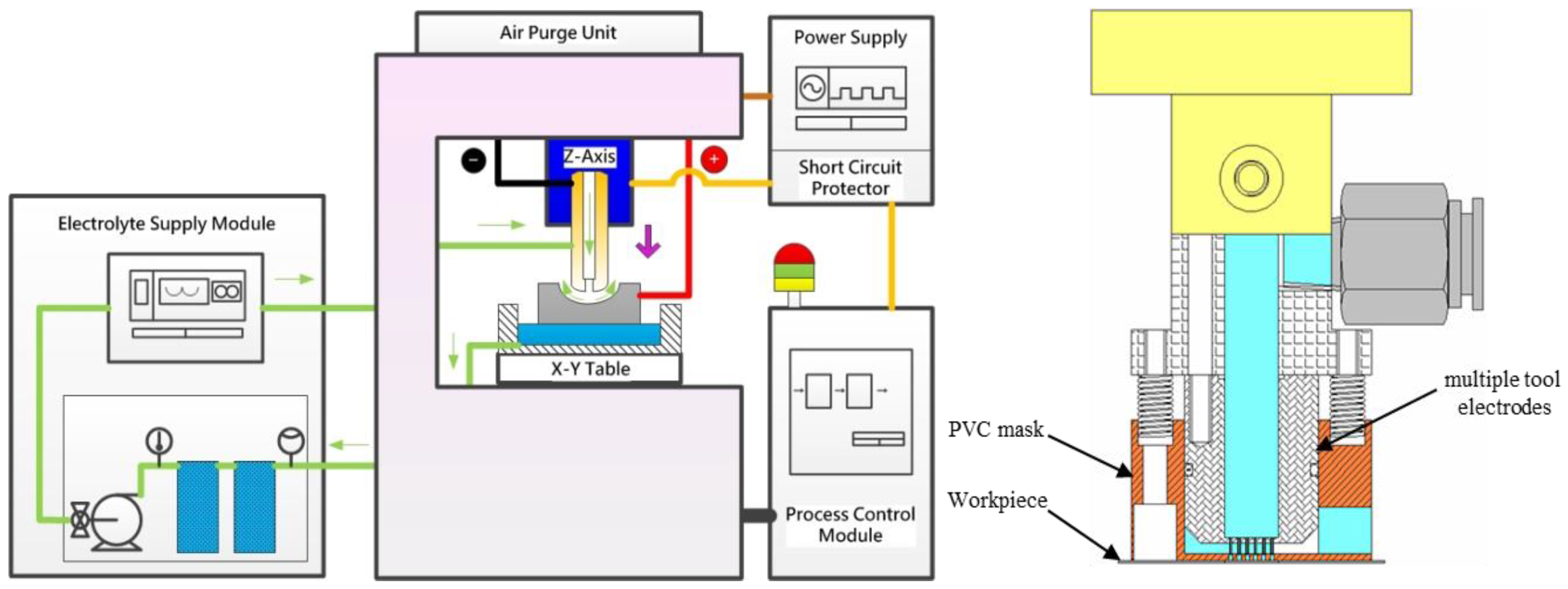
Figure 1 schematically depicts the μ-ECM experimental setup. The system consists of a three-dimensional movement device, a small-scale power supply of 100 A, a hydraulic pump for electrolyte delivery and a filtration system for slag removal. The feeding system is controlled by a PC-Based Computer Numerical Controlled Controller, a RTX real-time windows kernel program, and a motion card that drives the linear motor precisely. A pulse generator supplied a periodic current to the experimental model. A digital oscilloscope ensured that the pulse generator produced a rectangular waveform with accurate amplitude. If the tool feed rates were excessive, the tool would contact the workpiece and cause a short circuit; thus, an oscilloscope was employed to detect any short circuits. Whenever the oscilloscope detected a short circuit, a signal was sent rapidly to the PC and the tool was extracted automatically until the measured voltage returned to the applied voltage. The micro-array hole electrode module included the multiple nozzle tool electrodes, Polyvinyl Chloride (PVC) mask and tool fixture. The electrolyte was pumped to a multiple-electrode cell and exited through the small nozzle in the form of a free-standing jet directed towards the anode workpiece.

Other basic information and settings are shown as follows: the electrolyte velocity was 10 m/s at the outlet of the pump, the electrolyte temperature was 27 °C, the initial gap between the tool and the workpiece was 100 µm, the tool moving distance was 800 µm, the workpiece material was SUS 304, the electrolyte used was 10% wt. NaNO₃, the nominal diameter of the hole was 900 µm, and the depth of the hole was 500 µm. The voltage, pulse-on-time, and feed rate were used as the controllable process parameters, while the inner diameter of the micro-hole D_in and the outer diameter D_out were the measurable performances. 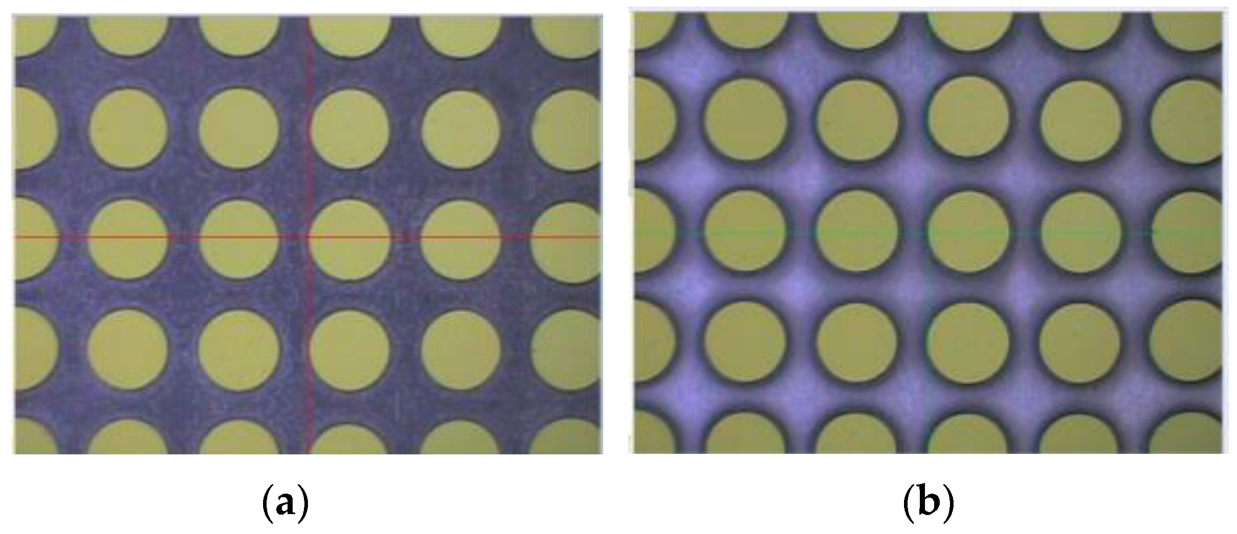Figure 2 shows the Charge Coupled Device (CCD) camera image of the array of holes drilled during the μ-ECM experiment.

3. Input-Output Modeling

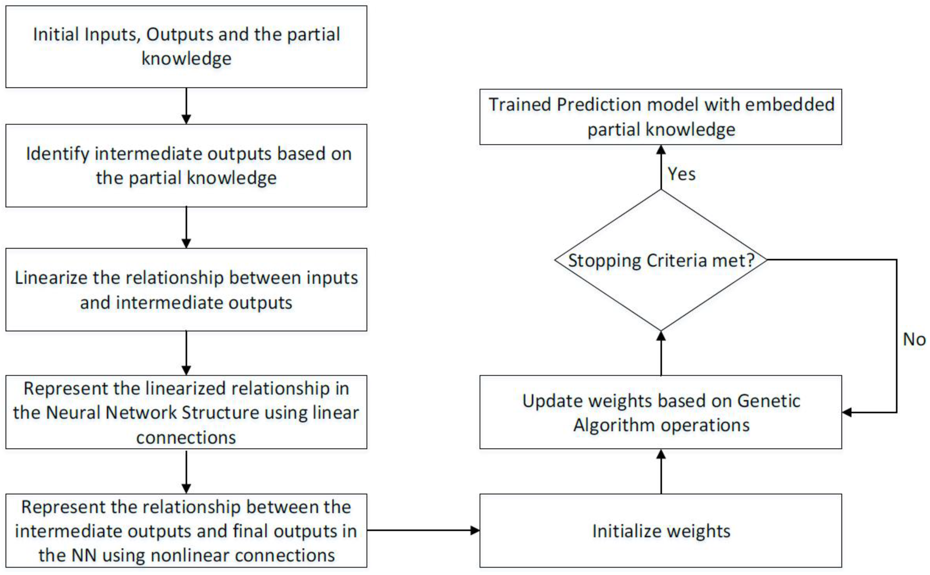
As stated earlier, current work in the literature focuses on mapping directly from the input process parameters to the KPIs. To attempt to increase the prediction accuracy, partial knowledge about the mechanisms of μ-ECM was embedded in the NN. This was accomplished by finding some intermediate outputs that are influenced by the inputs and are closely related to the outputs. The relationship between the inputs and intermediate outputs has been studied by researchers [11,12,13]. To embed this knowledge in the NN, the relationship between the inputs and the intermediate outputs was first linearized. This linearized relationship was represented in the NN as linear weighted connections between the inputs and the first hidden layer, where the outputs from the first hidden layer represent intermediate outputs. Additional hidden layers were then added to the NN, which connected the first hidden layer and the output layer where the connections were nonlinear. Once the NN structure with the embedded partial physical knowledge was established, the weights of the NN could be trained using any gradient-based or metaheuristic algorithm. The flowchart of the proposed idea is shown in Figure 3.

The following assumptions were made to simplify the relationship between the inputs and the intermediate outputs: the electrochemical gap between the tool (cathode) and the workpiece (anode) was assumed to be constant for one set of input parameters (voltage, feed and pulse-on-time). The transient response was ignored, and the whole process was assumed to be in steady state. The electrolyte conductivity was assumed to be constant because the refill tank was significantly large in comparison with the electrolyte involved in the machining process. Therefore, the active ion in the electrolyte could be assumed to be constant. Since the tool was not coated with insulation material, we assumed the electrical field was uniform around the tool. Eddy flow was neglected in the inter-electrolyte gap and the horizontal velocity was assumed to be constant. In addition, friction and heat transfer were not considered in establishing the physical model due to the high electrolyte flow rate and the low surface roughness.

In this paper, four intermediate outputs were determined to be the most influential on the outputs, i.e., the current density, the inter-electrode gap, the void fraction, and the material removal rate. According to McGeough [12], the current density in μ-ECM can be calculated using Equation (1)

$$J=\frac{I}{A}=\frac{K_{e}V}{h}$$

(1)

where $I$ denotes the current, $A$ is the area where the current is applied to, ${\kappa }_e$ represents the electrolyte conductivity which is assumed to be constant, $V$ is the voltage applied, and $h$ is the inter-electro gap width which is set to constant in the assumption. Therefore, the intermediate output $J$ has a linear relationship with the input parameter which can be described using Equation (2)

$$J=C_1\times V$$

(2)

where $C_1$ is a coefficient related to the electrolyte conductivity ${\kappa }_e$ and the inter-electrode gap $h$. In addition, the equilibrium gap was derived in [12] using Equation (3). Kozak reported that the pulse time p will influence the equilibrium gap and material removal rate in [11]. The relationship can be described using an exponential function with respect to the pulse time as shown in Equation (3)

$$h_e=\frac{MV{e}^{cp}}{f}$$

(3)

where $M$ is a machining parameter related to the atomic numbers and valencies of the elements constituting the workpiece, the electrolyte conductivity, Faraday’s constant and the density of the workpiece; $V$ is the voltage applied; $f$ is the feed rate of the electrode; c is a constant; and p is the pulse-on-time. Since the workpiece was composed of different materials, the overall atomic number and valence needed to be determined. Two methods are widely used in the derivation. One is the ‘percentage by weight’ method and the other is the ‘superposition of charge’ method [12]. In this paper, the superposition of charge method was used to obtain the atomic number and valence of stainless steel 304. Because the ECM process involves a pulsed voltage input, some corrections needed to be made to compensate for the transient state caused by the short pulses. Equation (3) can be linearized using a first-degree Taylor approximation and can be given by:

$$h_e=C_2+C_3\times V+C_4\times f+C_5\times p$$

(4)

where $C_2$, $C_3$, $C_4$, $C_5$ are the linearization coefficients and $p$ is the pulse time.

Thorpe derived the relationship of the void fraction based on the separation of the electrolyte flow within the electrochemical gap, the fundamental kinematic equation and the transport equations [13]. He also proposed that the ECM process can be characterized by four dimensionless parameters. Based on Thorpe’s derivation and the assumption made previously, the void fraction can be described using Equation (5)

$$\alpha =\frac{\frac{{\lambda }_a{\rho }_{a}Lf}{{\rho }_g{C}^{*}{h}_e{V}_0}}{(1+\frac{{\rho }_0{\lambda }_g+{\rho }_g-{\rho }_g{\lambda }_g}{{\rho }_g{C}^{*}})(\frac{{\rho }_{a}Lf}{{\rho }_0{h}_e{V}_0})}$$

(5)

where ${\lambda }_a$, ${\lambda }_g$ are the electrochemical equivalents for the anode material and the gas; ${\rho }_a$, ${\rho }_g$, ${\rho }_0$ are density of the anode material, gas and electrolyte, respectively; $C^{*}$ is a constant; $L$ is the distance from the outer diameter of the electrode to the bottom corner of the machined hole; $f$ is the feed rate; and $V_0$ is the inlet electrolyte velocity. Equation (5) can also be linearized into Equation (6) using a first-degree Taylor approximation as:

$$\alpha =C_6+C_7\times f+C_8\times V$$

(6)

The last intermediate output is the material removal rate which can be described by Equation (7) with consideration of the pulsed voltage derived from [11],

$$MRR=\frac{b\times thickness\times f\times e^{b^{*}\times p}}{travel\_d}$$

(7)

where $b$ and $b^{*}$ are the correction factors and travel, d is the travel distance from of the tool from beginning of the machining process to the end. The linearized form of Equation (7) is shown next as Equation (8)

$$MRR=C_9+C_{10}\times f+C_{11}\times p$$

(8)

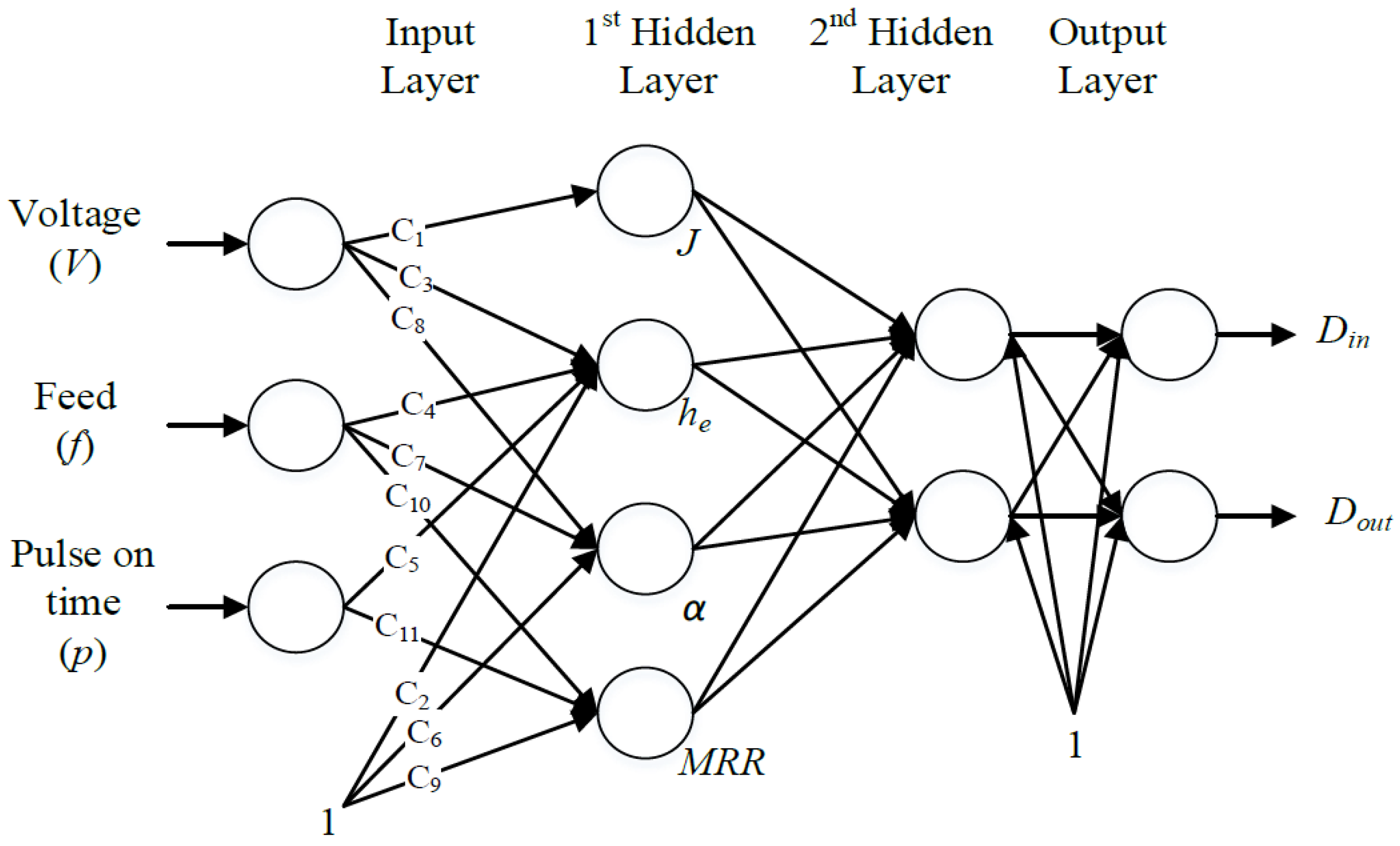
The four desired intermediate outputs described by Equations (2), (4), (6) and (8) were calculated using the experimental data obtained from [7]. The relationships developed in Equations (2), (4), (6), and (8) were embedded in the NN as linear connections between the inputs and the hidden neurons of the first hidden layers. Since there is no understanding of the relationship between the intermediate outputs and the final outputs, another hidden layer was used. The connection between the first hidden layer and the second hidden layer as well as the second hidden layer to the output player was nonlinear. The proposed idea is shown in Figure 3. The training procedure for the embedded physics model is shown in Figure 4. The constants C₁ through C₁₁ were treated as the weights of the linearized NN, as shown in Figure 4.

To determine whether the NN with the embedded partial knowledge would have higher prediction accuracy than a pure NN model, the weights of the proposed NN structure were first trained using the genetic algorithm (GA) [14]. The available experimental data (see Appendixas divided into training (70%), validation (15%), and testing (15%) sets. The training data sets were used to training the weight values, while the validation data sets were used to ensure that the weight values did not over-fit to the training data set. Once the NN had been trained, its prediction accuracy was measured by using it to predict the outputs of the testing data set. During the training procedure, the aim of the GA was to minimize the mean squared error (MSE), given by Equation (9), of the training data set. At each iteration of the training procedure, the MSE of the validation data set was also calculated and the set of weights that provided the smallest MSE for the validation data set were used as the final weight values.

$$\mathrm{Mean}\mathrm{squared}\mathrm{error}=\frac{1}{n}{\displaystyle \sum _{i=1}^n{(y_{a,i}-y_{p,i})}^2}$$

(9)

where $y_{a,i}$ is the actual output of the ith data set and $y_{p,i}$ is the predicted output of the pth data set.

4. Results

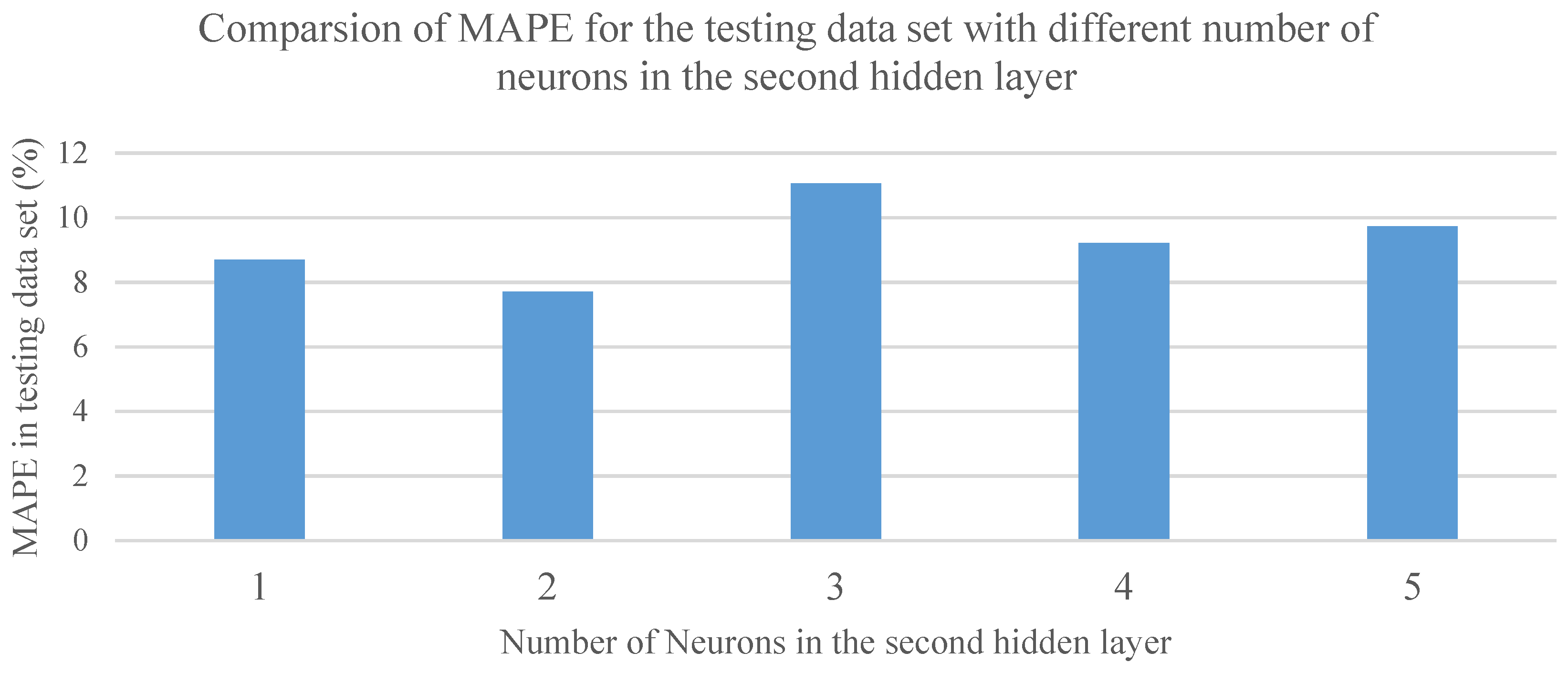
Since no theoretical guideline for choosing the number of neurons in the second hidden layer exists, a trial-and-error–based method was used to determine the number of neurons in the second hidden layer. In the trial-and-error–based method, the number of neurons in the second hidden layer was varied and a NN was trained to predict the outputs for the testing data set. For each NN structure, 10 simulations were run with the same training, validation, and testing data sets and the Mean Absolute Percentage Error (MAPE) of the testing data set was used to determine the best NN structure for the hybrid model. Figure 5 shows the MAPE obtained for the test set using different numbers of neurons in the second hidden layer.

It can be observed from Figure 5 that the hybrid structure that had two neurons in the second hidden layer had the best prediction accuracy for the testing data set.

During the training procedure, the following settings for the GA were used: a population size of 200, an iteration limit of 100, and a crossover rate of 0.5. The results obtained using the proposed NN structure were also compared to pure NNs where the outputs were directly mapped to from the inputs. In pure NN models, the number of hidden neurons in the first hidden layer was altered to find the best pure NN structure. The prediction accuracies of the NN with embedded partial knowledge and the pure NN were compared by looking at the mean absolute percentage error (MAPE) of the testing data set. To accurately compare the different types of NN models, five different simulations were performed and, in each simulation, the training, validation, and testing data sets were changed.

Table 1. Comparison of the MAPE obtained for the test set using the pure NN model with a 3-1-2 structure and the NN model with embedded knowledge.

Simulation #	MAPE Obtained Using NN Model with Embedded Knowledge (%)	MAPE Obtained Using Pure NN Model with 3-1-2 Structure (%)	% Improvement
1	8.32	8.72	4.59
2	10.01	10.93	8.42
3	10.54	11.15	5.46
4	8.83	9.04	2.36
5	8.69	9.24	5.93

,

Table 2. Comparison of the MAPE obtained for the test set using the pure NN model with a 3-2-2 structure and the NN model with embedded knowledge.

Simulation #	MAPE Obtained Using NN Model with Embedded Knowledge (%)	MAPE Obtained Using Pure NN Model with 3-2-2 Structure (%)	% Improvement
1	8.32	8.87	6.17
2	10.01	11.12	9.99
3	10.54	11.84	10.97
4	8.83	9.07	2.71
5	8.69	9.76	10.92

,

Table 3. Comparison of the MAPE obtained for the test set using the pure NN model with a 3-3-2 structure and the NN model with embedded knowledge.

Simulation #	MAPE Obtained Using NN Model with Embedded Knowledge (%)	MAPE Obtained Using Pure NN Model with 3-3-2 Structure (%)	% Improvement
1	8.32	8.62	3.42
2	10.01	10.55	5.11
3	10.54	12.20	13.55
4	8.83	9.85	10.36
5	8.69	10.36	16.08

and

Table 4. Comparison of the MAPE obtained for the test set using the pure NN model with a 3-4-2 structure and the NN model with embedded knowledge.

Simulation #	MAPE Obtained Using NN Model with Embedded Knowledge (%)	MAPE Obtained Using Pure NN Model with 3-3-2 Structure (%)	% Improvement
1	8.32	8.79	5.35
2	10.01	10.64	5.90
3	10.54	11.55	8.74
4	8.83	9.18	3.84
5	8.69	9.98	12.89

compare the MAPEs obtained for the test set using the NN model with embedded knowledge and the pure NN model.

As can be seen from Table 1, compared to the pure NN model with a 3-1-2 structure, i.e., three input neurons, one hidden neuron, and one output neuron, the NN model with embedded knowledge had a better prediction accuracy ranging from 2.36% to 8.42%. Compared to the pure NN model with a 3-2-2 structure, the NN model with embedded knowledge had a better prediction accuracy ranging from 2.71% to 10.97%. The NN model with embedded knowledge was 3.42%–16.08% better than the pure NN model with a 3-3-2 structure, and compared to the pure NN model with a 3-4-2 NN structure, the NN model with embedded knowledge was better by 3.84%–12.89%.

5. Conclusions

In this paper, a new approach was introduced to increase the prediction accuracy of NNs. Rather than directly mapping from the inputs of the process to the outputs, as is the case in current NN prediction models, partial knowledge about the mechanisms of the process was embedded in the NN in the form of the NN structure. To validate the proposed approach, the hybrid model was used on a case study of μ-ECM. Four different intermediate outputs, whose relationships to the inputs were known and were considered to have an impact on the final outputs, were obtained based on studies from other literature. The relationships between the inputs and the intermediate outputs were linearized and these relationships were then embedded in the NN by using linear weighted connections between the input layer and the first hidden layer. Due to the limited understanding of the connection between the intermediate layer and output layers, the relationship between the two layers was represented using non-linear weighted connections. A trial and error based method was used to determine the optimized neuron numbers in the non-linear hidden layer. Then, the NN model with embedded partial physical knowledge was trained using the μ-ECM experiment data with 70% of data for training, 15% of the data for validation and 15% of the data for testing. After sufficient training and absence of overfitting, the input process parameters were fed into the embedded model to predict the D_in and D_out, and the MAPE for the test set was obtained to compare its performance with the traditional two-hidden-layer NN with different structures. When compared to pure NN models, the MAPEs for the test sets obtained using the NN models with embedded knowledge were better by 3.42%–16.08%. The physics-embedded NN model showed higher prediction accuracy over that of the pure NN model. It was also shown that the level of accuracy improvement is affected by the structure of the NN model.