A Novel Modelling Approach for Condensing Boilers Based on Hybrid Dynamical Systems

Abstract

Condensing boilers use waste heat from flue gases to pre-heat cold water entering the boiler. Flue gases are condensed into liquid form, thus recovering their latent heat of vaporization, which results in as much as 10%–12% increase in efficiency. Modeling these heat transfer phenomena is crucial to control this equipment. Despite the many approaches to the condensing boiler modeling, the following shortcomings are still not addressed: thermal dynamics are oversimplified with a nonlinear efficiency curve (which is calculated at steady-state); the dry/wet heat exchange is modeled in a fixed proportion. In this work we cover these shortcomings by developing a novel hybrid dynamic model which avoids the static nonlinear efficiency curve and accounts for a time-varying proportion of dry/wet heat exchange. The procedure for deriving the model is described and the efficiency of the resulting condensing boiler is shown.

1. Introduction

It is a well-known fact that energy used by buildings is responsible for over a third of Europe and US global energy consumption and carbon dioxide (${\mathrm{CO}}_2$) emissions which heavily contribute to climate change [1]. One way to achieve reduced energy consumption in the building sector is via better control, which has been estimated to provide a 10%–40% energy saving potential [2]. As every control design starts from a good knowledge of the system to be controlled, in this work we will focus on the development of a novel hybrid dynamic model for a very crucial equipment of today’s buildings: condensing boilers. The relevance of the condensing boiler case arises from the fact that, with respect to total heating, ventilating and air conditioning (HVAC) operations, boilers are estimated to contribute to 85% of the energy consumption and 67% of the CO${}_2$ emissions [3]. Condensing boilers are increasingly being adopted and due to their typical bimodal behavior (condensing, noncondensing mode), modeling and control of condensing boilers is nontrivial and not completely explored yet. The exit flue gas temperature of a conventional gas fired boiler is usually high and a great amount of heat energy is lost to the environment. Condensing boilers aim at recovering both, the sensible heat and the latent heat by adding a condensing heat exchanger (see Figure 1). Return water of the heating system is used as the cooling medium of the condensing heat exchanger. As such, condensing boilers achieve better performances when return temperatures from the heating system are lower and above all, when these temperatures are below the dew temperature of the flue gas: this allows recovering the latent heat of water vapor in the flue gas, so as to achieve significantly higher efficiency levels than conventional boilers. The key point is maintaining a high difference between delivery and return temperature. When this condition is not maintained, the boiler will operate in a non condensing mode [4].

The development of analytical boiler models is the base of optimal boiler design and monitoring: in [5] a simple model was developed to predict the seasonal efficiency of condensing boilers based on the efficiency at full load evaluated at return water mean temperature. In [6] an analytical model of heat and mass transfer processes in a flue gas condensing heat exchanger system was developed to predict the heat transferred from flue gas to cooling water and the condensation rate of water vapor in the flue gas. The main purpose of these models is to predict the boiler efficiency according to certain choices of design parameters. In fact, the use of these models allows the computation of relevant variables like flue gas exit temperature, cooling water outlet temperature, water vapor mole fraction, and condensation rate of water vapor using the analytic model. Other condensing boiler models have been developed in [7,8,9,10,11]. Despite the numerous modeling approaches, we can still identify the following shortcomings in existing models:

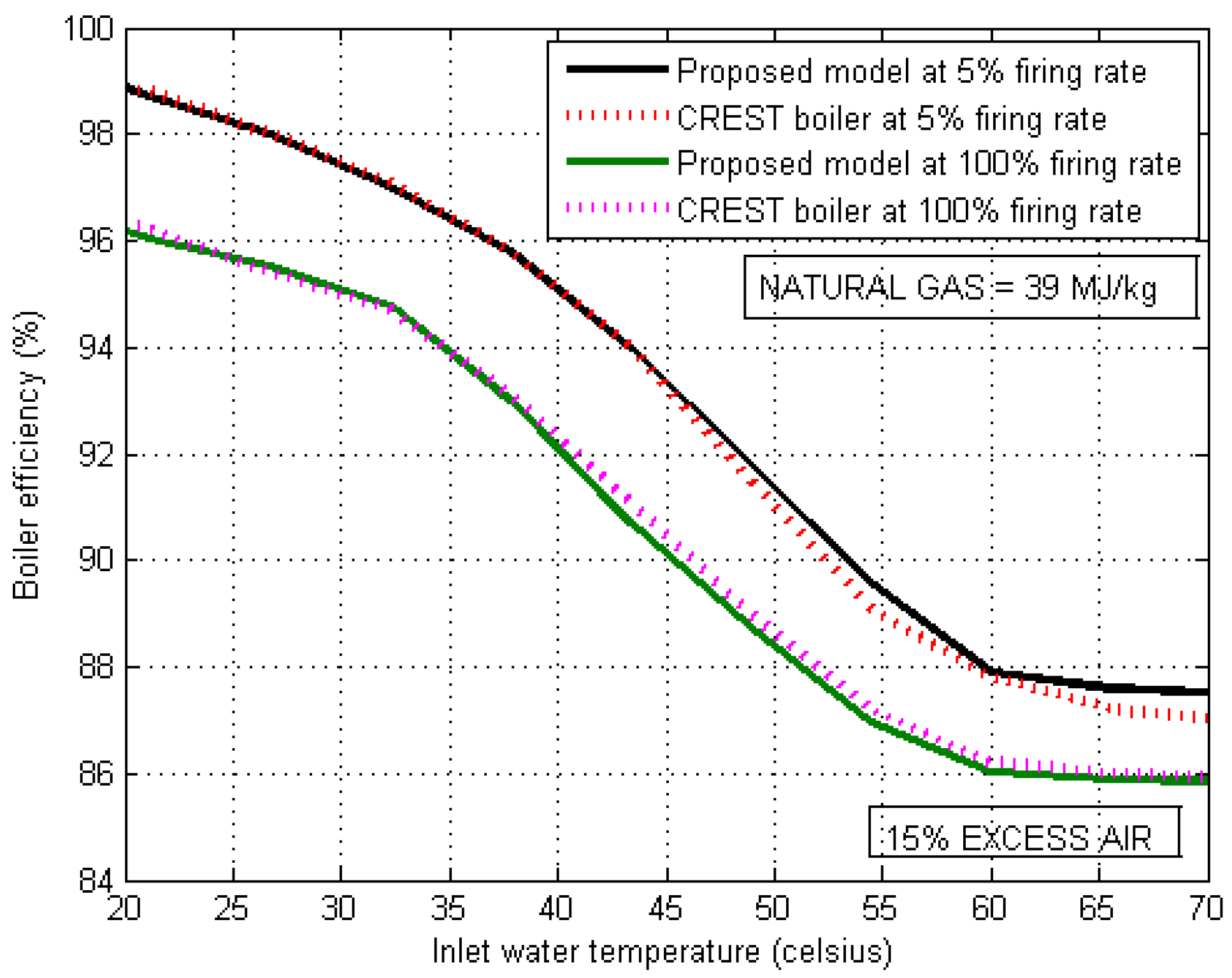
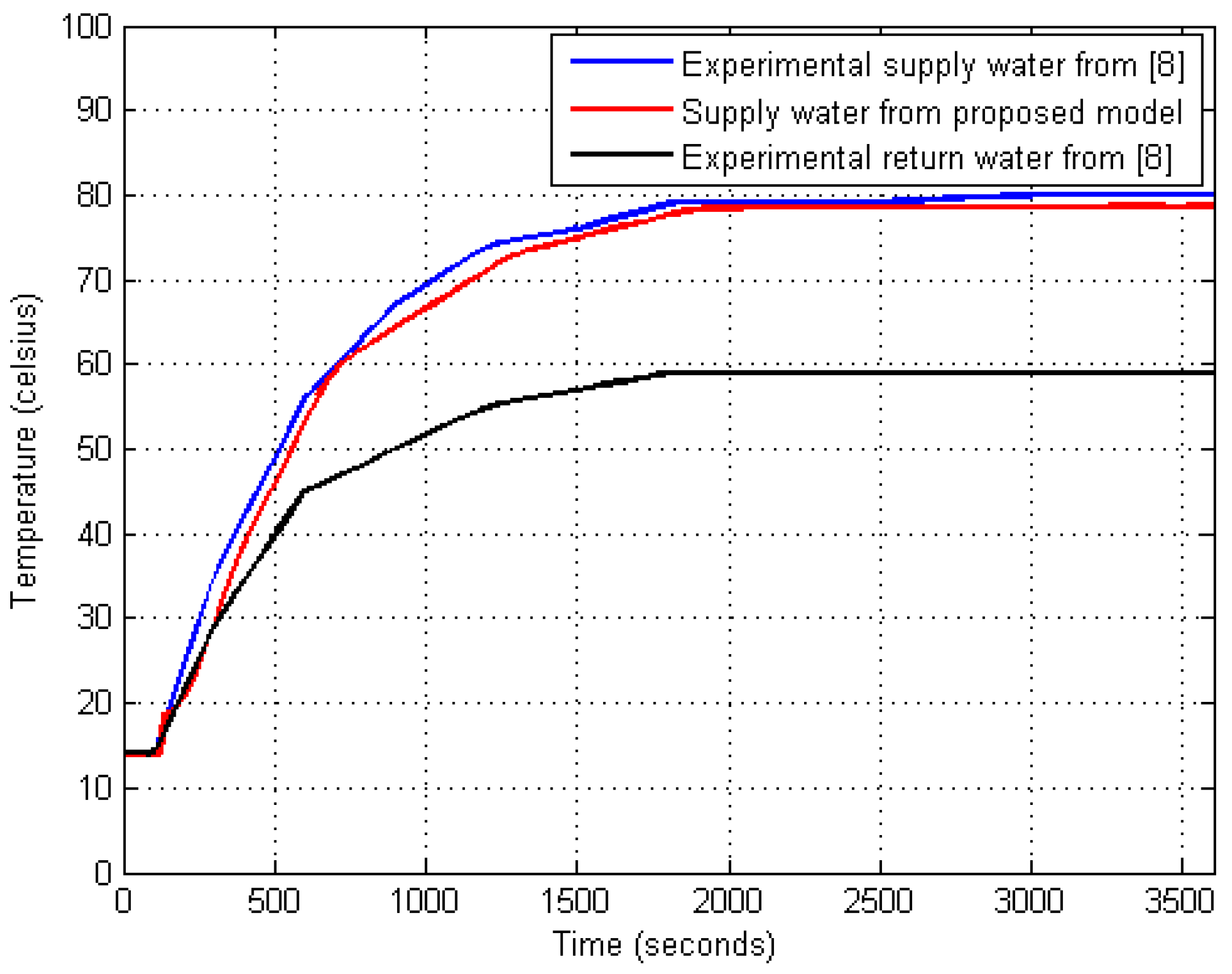
• Thermal dynamics are either neglected or oversimplified with a nonlinear efficiency curve followed by two point thermal nodes. It is important to point out that the efficiency curve is always calculated by installers and specifiers of domestic/commercial heating systems, at steady-state. Therefore, it might not be able to represent the dynamics of the boiler.
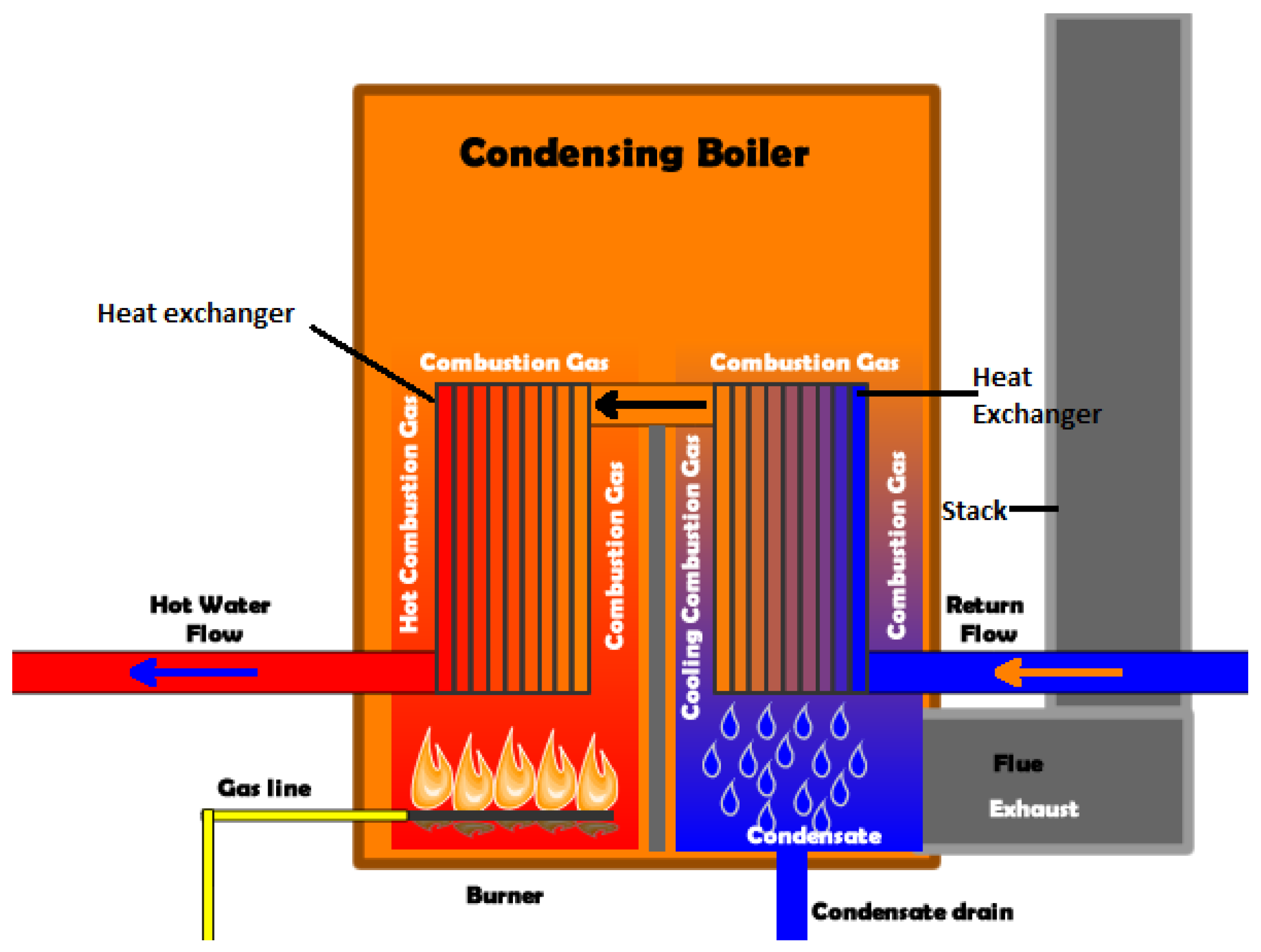
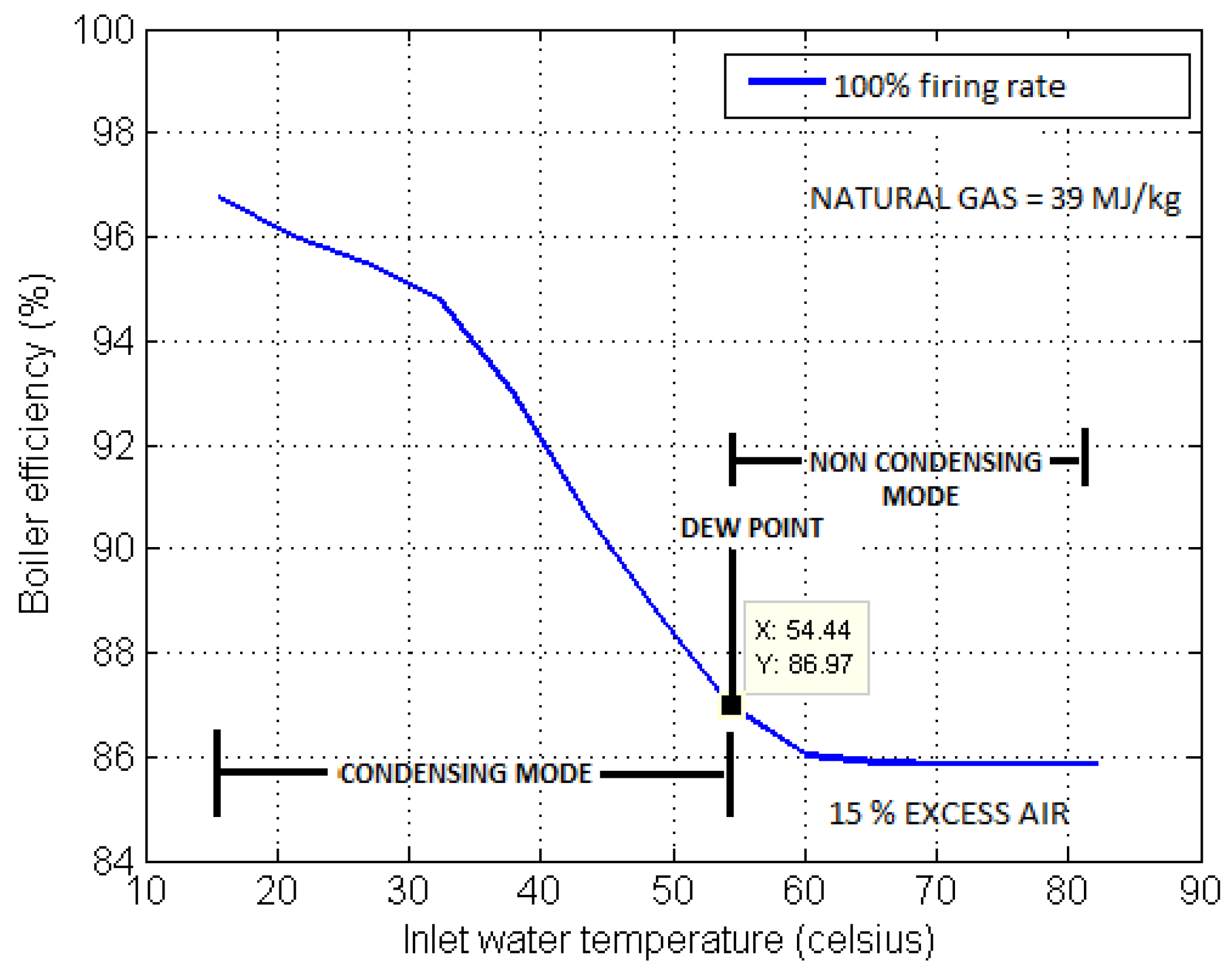
• The condensing/noncondensing behavior is either neglected or oversimplified with two heat exchangers with a fixed proportion of dry/wet heat exchange. Required is a model that is capable of capturing possible time-varying proportions of dry/wet heat exchange occurring during dynamical behavior.

With this work we aim at overcoming these shortcomings. We develop a model which is able to both, capture highly dynamic heat transfer behavior and describe the proportion of dry/wet heat exchange according to the temperature of the return water. Due to its hybrid nature, the proposed model paves a way for hybrid control of smart heating systems. In recent years this has been a fruitful line of research, among the main contributions being the following [12,13,14,15,16,17,18]. In fact, boiler operation is only one part of a bigger control system which regulates energy supply and demands in buildings: different supervisory control architecture based on model predictive controllers, rule-based strategies or other multiobjective optimization techniques [19,20,21,22,23].

The rest of the paper is organized as follows: Section 2 gives the basics of boiler functioning and the heat exchanges involved during operation. Section 3 develops a hybrid dynamic model of the condensing boiler. In Section 4 the simulation results are presented and analyzed and Section 5 concludes the work.

2. Boiler Operation and Involved Heat Exchanges

This section focuses on the basics of the condensing boiler functioning and the various heat transfer phenomena involved. As shown in Figure 1 the key boiler components involved are the burner, combustion chamber, two portions of the heat exchanger and stack. The burner mixes the fuel and oxygen together and, with the assistance of an ignition device, provides a platform for combustion. The combustion reaction taking place in the combustion chamber with 15% excess air is given as:

$$\begin{array}{c}\hfill C{H}_4+\frac{2}{0.85}{O}_2+\frac{7.56}{0.85}{N}_2\to C{O}_2\left(g\right)+2H_{2}O\left(g\right)+8.89N_2\left(g\right)+0.353O_2\left(g\right)\end{array}$$

(1)

The combustion gas consists of the products of Equation (1) in the volume composition given by: 8.17% of $C{O}_2$ (Carbon dioxide), 16.33% of $H_{2}O$ (Water Vapor) , 2.88% of $O_2$ (Oxygen) and 72.62% of $N_2$ (Nitrogen). The combustion gas/exhaust gas moves through the heat exchanger transferring heat to the cold return water in the process. An idealized heat exchanger involving heat exchange of combustion gas on one side and water on the other side can be described as shown in Figure 2.

The heat exchanger consists of four zones namely combustion gas, extended surface, tube wall and water. It is assumed that the thermal resistances of the tube wall and extended surface materials can be neglected. The basis for the assumption is that thermal resistances of the tube wall and extended surface materials (cast steel or aluminium) can be neglected as compared to the thermal resistance of water and gas. Therefore, if the extended surface temperature gradient is accounted for by an effectiveness term, heat transfer from combustion gas will be with reference to extended surface temperature and the heat transfer from water will be with respect to tube wall surface temperature. The evolution of combustion gas temperature $T_a$ in (${}^{°}$C) is given by [24]:

$$\begin{array}{c}\hfill \frac{\partial T_a}{\partial t}=-\frac{w_a}{{\rho }_a{A}_{af}}\frac{\partial T_a}{\partial l}-\frac{h_o{D}_o}{C_a{\rho }_a{A}_{af}}(T_a-T_f)\end{array}$$

(2)

where the first term represents the heat exchange within the combustion gas side and the second term represents the heat exchange with the extended surface temperature $T_f$ in (${}^{°}$C). In Equation (2) $C_a$ is the thermal capacitance of the combustion gas in (kJ/kg${}^{°}$C), $w_a$ is the mass flow rate of the combustion gas with respect to equivalent free flow area in (kg/s), $h_o$ is the surface convection coefficient for the effective combustion gas side in (kW/m${}^2$ °C), $D_o$ is the combustion gas side perimeter of the heat transfer surface in (m), ${\rho }_a$ is the combustion gas density in (kg/m${}^3$) and $A_{af}$ is the effective free flow area on the combustion gas side in (m${}^2$). The evolution of water temperature $T_w$ in (${}^{°}$C) is given by [24]:

$$\begin{array}{c}\hfill \frac{\partial T_w}{\partial t}=\frac{w_w}{{\rho }_w{A}_{wf}}\frac{\partial T_w}{\partial l}-\frac{h_i{D}_i}{C_w{\rho }_w{A}_{wf}}(T_w-T_t)\end{array}$$

(3)

where the first term represents the heat exchange within the water side and the second term represents the heat exchange with the tube wall temperature $T_t$ in (${}^{°}$C). In Equation (3) $C_w$ is the thermal capacitance of water in (kJ/kg${}^{°}$C), $w_w$ is the mass flow rate of water with respect to equivalent free flow area in (kg/s), $h_i$ is the tube internal surface convection coefficient on the water side in (kW/m${}^2$ °C), $D_i$ is the water side perimeter of the heat transfer surface in (m), ${\rho }_w$ is the water density in (kg/m${}^3$) and $A_{wf}$ is the effective free flow area on the water side in (m${}^2$). The evolution of tube wall temperature is given by [24]:

$$\begin{array}{c}\hfill \frac{d{T}_t}{dt}=-\frac{h_i}{C_t{\rho }_t{d}_t}(T_t-T_w)-\frac{(T_t-T_f)}{C_t{\rho }_t{d}_t{R}_{tf}}\end{array}$$

(4)

where the first term represents heat exchange with the water temperature and the second term represents heat exchange with extended surface temperature. In Equation (4) ${\rho }_t$ is the density of tube wall material in (kg/m${}^3$), $C_t$ is the thermal capacitance of the tube wall material in (kJ/kg${}^{°}$C), $d_t$ is the tube wall thickness in (m) and $R_{tf}$ is the thermal resistance between tube wall and extended surface core in (m${}^2$ ${}^{°}$C/kW). The evolution of extended surface temperature is given by [24]:

$$\begin{array}{c}\hfill \frac{d{T}_f}{dt}=-\frac{h_o}{C_f{\rho }_f{d}_f}(T_f-T_a)-\frac{D_i}{C_f{\rho }_f{d}_f{R}_{tf}}(T_f-T_t)\end{array}$$

(5)

where the the first term represents heat exchange with the combustion temperature and the second term represents heat exchange with tube wall temperature. In Equation (5) ${\rho }_f$ is the density of extended surface material in (kg/m${}^3$), $C_f$ is the thermal capacitance of the extended surface material in (kJ/kg${}^{°}$C) and $d_f$ is the extended surface wall thickness in (m). Notice that Equations (2)–(5) are sensible heat balance equations.

Depending on the cold return water temperature, the condensing boiler operates in two modes, namely: condensing and non condensing modes. Correspondingly, there are two types of heat exchange (dry and wet heat exchange) involved in the heat exchanger which will be explained in the subsequent sections. A condensate drain is installed to collect the condensed water vapor. Hot water produced by a boiler is typically pumped through pipes and delivered to equipment throughout the building, which can include hot water coils in air handling units, service hot water heating equipment, and terminal units [25]. Flue gas exits the boiler through a stack.

Remark 1. 

Summarizing, all the temperatures are functions of both space and time. As such we end up with a set of partial differential Equations (2)–(5). In order to obtain a more tractable model, we perform a spatial discretization of Equations (2)–(5), which will result in a set of ordinary differential equations which are functions of time. A temporal discretization at this point is not necessary, because the resulting model can be easily handled by ordinary differential equation initial value problem solvers (e.g., implemented in MATLAB^®/Simulink^®).

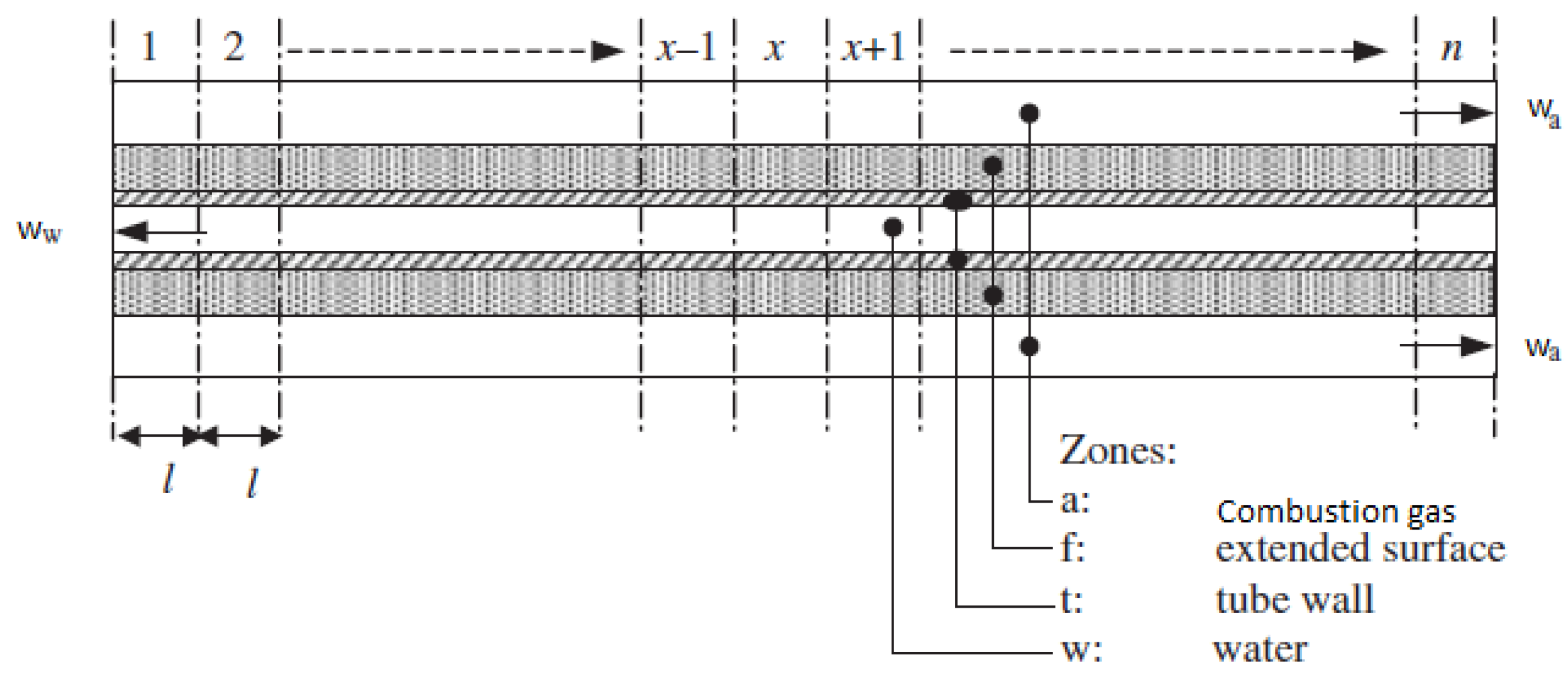
3. Dynamic Thermal Modeling

The partial differential equations of the sensible heat balance on the combustion gas side given by Equation (2) and water side given by Equation (3) are spatially discretized to obtain a model suitable for simulation and analysis. As shown in Figure 2 the heat exchanger can be discretized into n elements. The temperature of combustion gas, water, tube wall and extended surface has to be divided into smaller elements $T_{{a,w,t,f}_x}$ for x ∈ 1, 2, …, n, each one modeled as a separate state. Due to the fact that the inlet gas and the return water are inputs to the boiler and to the fact that the water is in counter flow to the gas flow, we use backward discretization in space for the water side and forward discretization in space for the flue gas side. For the non-condensing mode, the resulting equations are as follows:

$$\begin{array}{c}\hfill \frac{d{T}_{a_x}}{dt}=-\frac{w_a}{{\rho }_{a_x}{A}_{af}\Delta l}(T_{a_x}-T_{a_{x-1}})-\frac{h_o{D}_o}{C_a{\rho }_{a_x}{A}_{af}}(T_{a_x}-T_{f_x})\end{array}$$

(6)

$$\begin{array}{c}\hfill \frac{d{T}_{w_x}}{dt}=\frac{w_w}{{\rho }_w{A}_{wf}\Delta l}(T_{w_{x+1}}-T_{w_x})-\frac{h_i{D}_i}{C_w{\rho }_w{A}_{wf}}(T_{w_x}-T_{t_x})\end{array}$$

(7)

$$\begin{array}{c}\hfill \frac{d{T}_{t_x}}{dt}=-\frac{h_i}{C_t{\rho }_t{d}_t}(T_{t_x}-T_{w_x})-\frac{(T_{t_x}-T_{f_x})}{C_t{\rho }_t{d}_t{R}_{tf}}\end{array}$$

(8)

$$\begin{array}{c}\hfill \frac{d{T}_{f_x}}{dt}=-\frac{h_o}{C_f{\rho }_f{d}_f}(T_{f_x}-T_{a_x})-\frac{D_i}{C_f{\rho }_f{d}_f{R}_{tf}}(T_{f_x}-T_{t_x})\end{array}$$

(9)

Note that $T_{a_x}$ in (${}^{°}$C) is the state corresponding to the combustion gas temperature in element x, $T_{f_x}$ in (${}^{°}$C) is the state corresponding to the extended surface temperature in the element x, $T_{w_x}$ in (${}^{°}$C) is the state corresponding to the water temperature in the element x, $T_{t_x}$ in (${}^{°}$C) is the state corresponding to the tube wall temperature in the element x, $T_{w_{x+1}}$ in (${}^{°}$C) is the water temperature in the element $x+1$, ${\rho }_{a_x}$ in (kg/m${}^3$) is the density of combustion gas in the element x, $T_{a_{x-1}}$ in (${}^{°}$C) is the combustion gas temperature in the element $x-1$ and $\Delta l$ is the length of the element in (m). Notice that in Equation (6) the density of combustion gas varies from element to element as the boiler is a constant-pressure combustion system.

Reduced flue gas temperature is what causes condensation in a boiler. The point at which condensing will occur, also called the dew point of the products of natural gas combustion, is about 54.4 ${}^{°}$C [26]. Above this temperature, the moisture en-trained in flue products as water vapor will remain vaporized. The heat transfer phenomenon occurring under this condition is called dry exchange and the boiler is said to operate in non condensing mode. The (spatially discretized) heat transfer associated with the combustion gas, extended surface, tube wall and water during dry exchange are given by Equations (6)–(9).

Below 54.4 ${}^{°}$C, the water vapor will change phase and condense out of the flue products as liquid. When this phase change occurs, additional energy is released which is beyond the sensible heat of the flue products. In a boiler, this phase change occurs on a heating surface and the released energy transfers through the heating surface into the boiler water on the other side. By capturing this energy, which is lost out of the exhaust stack in a typical boiler, a condensing boiler gains in efficiency [26]. The higher efficiency in condensing boilers is due to the condensation of water vapor and the consequent use of latent heat to reheat the return water. Naturally, the products of combustion cannot be reduced in temperature to 54.4 ${}^{°}$C unless the heating surfaces in the boiler are also at temperatures less than or equal to 54.4 ${}^{°}$C. The only way to accomplish this is to have an entering boiler water temperature of less than or equal to 54.4 ${}^{°}$C. When, the return water temperature is less than or equal to 54.4 ${}^{°}$C the boiler is said to operate in condensing mode and the various heat transfer phenomenon occurring in this mode are called wet exchange. The (spatially discretized) heat transfer associated with the combustion gas, extended surface, tube wall and water during wet exchange are as follows:

$$\begin{array}{c}\hfill \frac{d{T}_{a_x}}{dt}=0\end{array}$$

(10)

$$\begin{array}{c}\hfill \frac{d{T}_{w_x}}{dt}=\frac{w_w}{{\rho }_w{A}_{wf}\Delta l}(T_{w_{x+1}}-T_{w_x})-\frac{h_i{D}_i}{C_w{\rho }_w{A}_{wf}}(T_{w_x}-T_{t_x})\end{array}$$

(11)

$$\begin{array}{c}\hfill \frac{d{T}_{t_x}}{dt}=-\frac{h_i}{C_t{\rho }_t{d}_t}(T_{t_x}-T_{w_x})-\frac{(T_{t_x}-T_{f_x})}{C_t{\rho }_t{d}_t{R}_{tf}}\end{array}$$

(12)

$$\begin{array}{c}\hfill \frac{d{T}_{f_x}}{dt}=-\frac{h_o}{C_f{\rho }_f{d}_f}(T_{f_x}-T_{a_x})-\frac{D_i}{C_f{\rho }_f{d}_f{R}_{tf}}(T_{f_x}-T_{t_x})+P_{cond}\end{array}$$

(13)

Observe that the flue gas temperature never goes below 54.4 ${}^{°}$C in which case, it would change phase while keeping its temperature constant, i.e. releasing an equivalent amount of heat so as to make the derivative of the flue gas temperature zero as shown in Equation (10). Therefore, the term $P_{cond}$ is calculated by assuming phase change of flue gas at constant temperature:

$$\begin{array}{c}\hfill P_{cond}=\frac{w_a}{{\rho }_{a_x}{A}_{af}\Delta l}(T_{a_x}-T_{a_{x-1}})+\frac{h_o{D}_o}{C_a{\rho }_{a_x}{A}_{af}}(T_{a_x}-T_{f_x})\end{array}$$

(14)

Remark 2. 

As the heat transfer equations are modeled in such a way that they can switch between dry or wet exchange as dictated by the cold return water temperature, the resulting model is hybrid: note that with “hybrid” we mean the concept, typically used in systems and control theory, of a hybrid dynamical system, i.e., a dynamic system that exhibits both continuous and discrete dynamic behavior—a system that can both flow and change regime. In particular, in the proposed approach, the change of regime is given by the flue gas reaching its dew point and changing phase. Thereby the proposed modeling approach captures the bimodal behavior exhibited by a typical condensing boiler.

The condensing boiler model has been built in MATLAB^®/Simulink^® and consists of five elements (n = 5) for the heat exchanger. The proposed modeling approach is modular so that the user can add and remove as many elements as desired, thereby making the discretization fine or coarse. In every element the heat exchange equations associated with the combustion gas, extended surface, tube wall and water are modeled in such a way that the heat transfer is governed by either dry exchange Equations (6)–(9), or wet exchange Equations (10)–(14) as dictated by the cold return water temperature. As the equations associated with dry and wet exchange are continuous functions of time, the resulting model is dynamic in nature.

4. Simulation Results and Analysis

The efficiency of the boiler is the main factor in the overall efficiency of a domestic/commercial central heating system. To calculate the efficiency it is essential to find the input power supplied and the output power. The input power $P_{in}$ in (kW) is given by:

$$\begin{array}{c}\hfill P_{in}=w_{ng}Hv\end{array}$$

(15)

where $w_{ng}$ is mass flow rate of the natural gas in (kg/s) and $Hv$ is heating value of natural gas in (kJ/kg). The output power is given by [27]:

$$\begin{array}{c}\hfill P_{out}=w_w{C}_w(T_{sup}-T_{ret})\end{array}$$

(16)

where $T_{sup}$ in (${}^{°}$C) is the hot supply water temperature leaving the boiler and $T_{ret}$ in (${}^{°}$C) is cold return water temperature entering the boiler. The ratio of $P_{out}$ and $P_{in}$ gives efficiency (%) of the condensing boiler:

$$\begin{array}{c}\hfill Efficiency=\frac{P_{out}}{P_{in}}·100\end{array}$$

(17)

To calculate the efficiency, steady state experiments are performed on the MATLAB^®/Simulink^® model of the condensing boiler. Initially mass flow rate of natural gas ($w_{ng}$), water mass flow rate ($w_w$) and return water temperature ($T_{ret}$) are kept fixed and a long simulation is run till steady state has been reached for $P_{out}$ and $P_{in}$. Once steady state is reached, $P_{out}$ and $P_{in}$ are calculated and consequently the efficiency is obtained using Equation (17). The steady state experiment is repeated for different values of return water temperature ($T_{ret}$) varying from 20 ${}^{°}$C to 70 ${}^{°}$C. The resulting efficiency is plotted as a function of return water temperature for two firing rates in Figure 3. In order to validate the model, we compared the efficiency of the proposed model with the efficiency of a real condensing boiler, namely a CREST Condensing Boiler by Lochinvar, whose efficiency curve and boiler parameters can be found in [28,29]. From Figure 3 we can observe a good match between the efficiency curves of a real boiler and the proposed model, thereby validating the model.

Analyzing the efficiency curve of the proposed model for 100% firing rate in Figure 4, it can be observed that the efficiency curve piece-wise resembles the typical condensing boiler efficiency curve given in literature [25]. Also from Figure 4 it can be seen that when return water temperature is below the dew point of exhaust gas, greater efficiency is achieved as expected for a typical condensing boiler. Above the dew point temperature, the boiler operates in non condensing mode and thus has lower efficiency and below the dew point temperature the boiler operates in condensing mode and consequently has a greater efficiency. Thus, the bimodal behavior of a condensing boiler is also exhibited in Figure 4.

Further, results of the evolution of supply water and the return water (inlet) temperature as a function of time of the dynamic model is shown in Figure 5. To be noted is that the return water temperature used for comparison is obtained from experimental data published in [8,10]. As evident from Figure 5, a close match is obtained between real data and the proposed model.

5. Conclusions

Modeling heat transfer phenomena in condensing boilers is crucial to improve their efficiency via better controls. In this work, we have shown a novel condensing boiler modeling approach with the following characteristics: contrary to the state of the art, the nonlinear efficiency curve is obtained via a hybrid modeling approach, rather than fixing a priori, a polynomial nonlinear efficiency curve (which is typically calculated at steady-state); contrary to the state of the art, the dry/wet heat exchange is modeled in a time varying proportion (depending on the return water temperature). The procedure for deriving the model has been described which results in a hybrid dynamical model. The efficiency of the resulting condensing boiler has been shown, highlighting the typical bimodal behavior of condensing boilers.

References

1. Pérez-Lombard, L.; Ortiz, J.; Pout, C. A review on buildings energy consumption information. Energy Build. 2008, 40, 394–398. [Google Scholar] [CrossRef]
2. Cockroft, J.; Samuel, A.; Tuohy, P. Development of a Methodology for the Evaluation of Domestic Heating Controls; Phase 2 of a DEFRA Market Transformation Programme Project, Carried Out Under Contract to BRE Environment; University of Strathclyde, Energy Systems Research Unit: Glasgow, UK, 2007. [Google Scholar]
3. Energy Saving Trust. Domestic Heating by Gas: Boiler Systems—Guidance For Installers and Specifiers; Central Heating System Specifications: England, UK, 2008; Available online: http://bpec.org.uk/downloads/CE30%20-%20Domestic%20heating%20by%20gas.pdf (accessed on 5 April 2016).
4. Lee, S.; Kum, S.M.; Lee, C.E. Performances of a heat exchanger and pilot boiler for the development of a condensing gas boiler. Energy 2011, 36, 3945–3951. [Google Scholar] [CrossRef]
5. Rosa, L.; Tosato, R. Experimental evaluation of seasonal efficiency of condensing boilers. Energy Build. 1990, 14, 237–241. [Google Scholar] [CrossRef]
6. Jeong, K.; Kessen, M.J.; Bilirgen, H.; Levy, E.K. Analytical modeling of water condensation in condensing heat exchanger. Int. J. Heat Mass Transf. 2010, 53, 2361–2368. [Google Scholar] [CrossRef]
7. Lazzarin, R.M.; Schibuola, L. Performance analysis of heating plants equipped with condensing boilers. Heat Recover. Syst. 1986, 6, 269–276. [Google Scholar] [CrossRef]
8. Ternoveanu, A.; Ngendakumana, P. Dynamic model of a hot water boiler. In Proceedings of the Climate 2000 Conference, Brussels, Belgium, 30 August 1997.
9. Lemort, V.; Rodriguez, A.; Lebrun, J. Simulation of HVAC Components with the Help of an Equation Solver; Solar Heating and Cooling Programme International Energy Agency: Liege, Belgium, 2008. [Google Scholar]
10. Makaire, D.; Ngendakumana, P. Thermal performance of condensing boilers. In Proceedings of the 32nd TLM-IEA Energy Conservation and Emission reduction in Combustion, Nara, Japan, 26–29 July 2010; pp. 1–11.
11. Aganovic, A. Analysis of Dynamical Behavior of the Boiler Room at Mechanical Engineering Faculty in Sarajevo in Standard Exploitation Conditions; Department of Energy and Process Engineering: Trondheim, Norway, 2013. [Google Scholar]
12. Chen, Q.; Finney, K.; Li, H.; Zhang, X.; Zhou, J.; Sharifi, V.; Swithenbank, J. Condensing boiler applications in the process industry. Energy Build. 2012, 89, 30–36. [Google Scholar] [CrossRef]
13. Michailidis, I.; Baldi, S.; Pichler, M.F.; Kosmatopoulos, E.B.; Santiago, J.R. Proactive control for solar energy exploitation: A german high-inertia building case study. Appl. Energy 2015, 155, 409–420. [Google Scholar] [CrossRef]
14. Lee, S.; Kum, S.M.; Lee, C.E. An experimental study of a cylindrical multi-hole premixed burner for the development of a condensing gas boiler. Energy 2011, 36, 4150–4157. [Google Scholar] [CrossRef]
15. Korkas, C.D.; Baldi, S.; Michailidis, I.; Kosmatopoulos, E.B. Intelligent energy and thermal comfort management in grid-connected microgrids with heterogeneous occupancy schedule. Appl. Energy 2015, 149, 194–203. [Google Scholar] [CrossRef]
16. Michailidis, I.; Baldi, S.; Kosmatopoulos, E.B.; Boutalis, Y.S. Optimization-based active techniques for energy efficient building control part II: Real-life experimental results. Available online: http://simonebaldi.my-board.org/wp-content/uploads/2014/06/BEE-RES2014PARTB.pdf (accessed on 5 April 2016).
17. Bojica, M.; Dragicevic, S. MILP optimization of energy supply by using a boiler, a condensing turbine and a heat pump. Energy Convers. Manag. 2002, 43, 591–608. [Google Scholar] [CrossRef]
18. Baldi, S.; Michailidis, I.; Ravanis, C.; Kosmatopoulos, E.B. Model-based and Model-free “Plug-and-Play” Building Energy Efficient Control. Appl. Energy 2015, 154, 829–841. [Google Scholar] [CrossRef]
19. Verhelst, C.; Logist, F.; Van Impe, J.; Helsen, L. Study of the optimal control problem formulation for modulating air-to-water heat pumps connected to a residential floor heating system. Energy Build. 2012, 45, 43–53. [Google Scholar] [CrossRef]
20. Baldi, S.; Karagevrekis, A.; Michailidis, I.; Kosmatopoulos, E.B. Joint energy demand and thermal comfort optimization in photovoltaic-equipped interconnected microgrids. Energy Convers. Manag. 2015, 101, 352–363. [Google Scholar] [CrossRef]
21. Tzivanidis, C.; Antonopoulos, K.; Gioti, F. Numerical simulation of cooling energy consumption in connection with thermostat operation mode and comfort requirements for the Athens buildings. Appl. Energy 2011, 88, 2871–2884. [Google Scholar] [CrossRef]
22. Korkas, C.D.; Baldi, S.; Michailidis, I.; Kosmatopoulos, E.B. Occupancy-based demand response and thermal comfort optimization in microgrids with renewable energy sources and energy storage. Appl. Energy 2016, 163, 93–104. [Google Scholar] [CrossRef]
23. Satyavada, H.; Babuska, R.; Baldi, S. Integrated dynamic modelling and multivariable control of HVAC components. In Proceedings of the 15th European Control Conference, Aalborg, Denmark, 29 June–1 July 2016. submitted.
24. Underwood, C.; Yik, F. Modelling Methods for Energy in Buildings; Blackwell Publishing Ltd.: Hoboken, NJ, USA, 2004. [Google Scholar]
25. BetterBricks. Boilers Introduction How Boilers Work. Available online: http://betterbricks.com/sites/default/files/operations/om_of_boilers_final.pdf (accessed on 29 December 2015).
26. Riverside Hydronics. Condensing Boiler Operation and Appropriate Use. Available online: http://www.riversidehydronics.com/pdf%20documents/Tech%20Papers/condensing%20boiler%20operation%20and%20use.pdf (accessed on 29 December 2015).
27. Riverside Hydronics. First Law of Thermodynamics Summary. Available online: https://www.phy.duke.edu/rgb/Class/phy51/phy51/node59.html (accessed on 30 December 2015).
28. Green Shoots Controls. Available online: http://www.greenshootscontrols.net/?p=153 (accessed on 30 December 2015).
29. Lochinvar. CREST Condesing Boiler. Available online: http://www.lochinvar.com/products/default.aspx?type=productline&lineid=177 (accessed on 31 December 2015).
Figure 1. Condensing boiler.
Machines 04 00010 g001
Figure 2. Ideal heat exchanger (edited from [24]).
Machines 04 00010 g002
Figure 3. Effect of return (inlet) water temperature on efficiency of condensing boiler.
Machines 04 00010 g003
Figure 4. Effect of return (inlet) water temperature on efficiency of condensing boiler.
Machines 04 00010 g004
Figure 5. Effect of supply and return water (inlet) temperature as a function of time.
Machines 04 00010 g005