1. Introduction
Wind turbines of the megawatt size are expensive, and hence, their overall availability must be high to optimize the energy generation, thus reducing the cost of energy. In the same way, wind turbine downtime must be minimized. This key feature can be achieved by introducing fault detection and isolation (FDI) systems. In the related state-of-the-art, the fault detection schemes for industrial wind turbines can be quite conservative. For example, turbines are simply turned off after minimal faults to wait for service. Consequently, there is a need for an effective FDI for improving wind turbine working conditions, even though it might lead to limited power production in the case of faults. In the last few years, some works have been proposed on wind turbine FDI.
As an example [
1], presented a Kalman filter-based diagnosis system for detecting faults in the blade root bending moment sensors. An unknown input observer was designed for the detection of sensor faults around the wind turbine drive train in [
2]. On the other hand, in [
3], active and passive fault tolerant control schemes are considered. More attention has been drawn on wind turbine electrical conversion systems. Some relevant examples can be found in [
4], where observer-based solutions for sensor fault detection are presented. In [
5], a fault detection and reconfiguration scheme for a doubly-fed wind turbine converter is shown.
Comparisons of the considered fault diagnosis schemes for wind turbine applications are beneficial to find the most effective methodology. In [
6], a wind turbine benchmark was presented, which was proposed for both FDI and FTCsolution comparisons. This benchmark model described a realistic three-blade horizontal variable speed wind turbine with a full-scale converter coupling, and it will be considered in the present study. Several FDI strategies were proposed in the recent literature for this specific benchmark [
6]. In particular, the most effective FDI approaches were based on support vector machines with a Gaussian kernel [
7], banks of estimators [
8], up-down counters for a redundant residual decision [
9], combined observer/Kalman filters [
10] and automatically generated fault models [
11].
This paper proposes a data-driven FDI approach, based on identified fuzzy residual generators, which is applied to the benchmark proposed in [
6]. To this aim, the key contributions of the presented study are remarked in as follows. First, the system complexity may not require the design of a sophisticated analytical model of the residual generators. In fact, as shown in this work, a method relying on fuzzy models is proposed, thus obviating the derivation of purely nonlinear mathematical models of the residual functions. Note that the advantages of model-based approaches with respect to data-driven solutions depend on the features of the model under diagnosis, as described, e.g., in [
12,
13]. For the first time, the suggested methodology is applied to the wind turbine benchmark. Secondly, residual generators in the form of fuzzy models are considered instead of purely nonlinear observer or filter functions. Again, for the first time, the authors have proposed here the design of these residual generators with application to the wind turbine benchmark. Third, by exploiting the failure mode and effect analysis described in the following, both the fuzzy identification and the fault isolation tasks are enhanced, without using complicated unknown input or disturbance decoupling approaches, as addressed, e.g., in [
12,
13].
This paper suggests the use of fuzzy logic, since it seems the natural tool for handling complicated and uncertain conditions [
14,
15] that, in general, are not available to the designer. The additional benefits of fuzzy logic in connection with errors-in-variable (EIV) identification techniques include its simplicity and its flexibility [
16,
17]. Fuzzy logic can model nonlinear functions with arbitrary complexity. Fuzzy models, called fuzzy inference systems (FIS), consist of a number of conditional “IF-THEN” rules. For the designer, these rules are easy to build, and as many rules as necessary can be supplied to describe the system adequately with arbitrary accuracy (although typically, only a moderate number of rules are needed). In fuzzy logic, unlike standard conditional logic, the truth of any statement is a matter of degree. FIS relies on membership functions to explain how to calculate the correct value between zero and one. The degree to which any fuzzy statement is true is denoted by a value between zero and one. Not only do the rule-based approach and flexible membership function scheme make fuzzy systems straightforward to create, but they also simplify the design of systems and ensure that you can easily update and maintain the system over time [
15].
As described in the following, the paper suggests the use of the Takagi–Sugeno (TS) model [
18], whose parameters are obtained via the identification procedure proposed in [
16,
17]. This procedure is based on the EIV identification strategy relying on the Frisch scheme, which assumes that the input and output data are affected by noise, thus providing an unbiased parameter estimation. The diagnosis approach being evaluated has also an important implication on the use of on-line diagnosis tools once the wind turbine is under customer operation. Therefore, the further contribution of the study regards the robustness and reliability analysis of the proposed FDI scheme. The effectiveness of the proposed strategy is verified using data sequences acquired from the wind turbine benchmark. Realistic conditions and comparisons with different fault diagnosis approaches have been considered to validate the proposed methodology. Note that the wind turbine simulator exploited in this study was modified by the authors, and the working conditions can be different from the ones shown in [
6], since it was oriented toward the assessment of the robustness and the reliability of the considered FDI schemes. Moreover, with respect to previous works by the same authors, this paper aims at describing the comprehensive data-driven approach to wind turbine FDI and its extended comparisons with different FDI strategies applied to the same case study.
Finally, the paper has the following structure.
Section 2 briefly recalls the wind turbine benchmark.
Section 3 addresses the strategy using the EIV identification approach exploited for obtaining the fuzzy models, which are used as residual generators for the design of the FDI strategy. The proposed FDI methodology is presented in
Section 4. The results achieved, which are summarized in
Section 5, show the performances of the fault diagnosis scheme, validated on the data directly acquired from the benchmark, and compared also with different methods.
Section 6 ends the paper by highlighting the main achievements of the work, providing suggestions for further studies.
2. Wind Turbine Benchmark Description
The three-blade horizontal axis turbine considered in this paper works according to the principle that the wind is acting on the blades and moves the rotor shaft. In order to up-scale the rotational speed to the generator, a gear box is introduced. A more accurate description of the benchmark model can be found in [
6].
The rotational speed, and consequently, the generated power, is regulated by means of two controlled inputs: the converter torque and the pitch angle of the turbine blades. From the wind turbine system, a number of measurements can be acquired. is the rotor speed, the generator speed and the torque of the generator controlled by the converter, which is provided with the torque reference, . The estimated aerodynamic torque is defined as . This estimate clearly depends on the wind speed, which is not a very accurate measurement.
The wind turbine model in the continuous-time domain is briefly recalled in this section. In particular, the aerodynamic model is defined as in Equation (
1):
where
ρ is the density of the air,
A is the area covered by the turbine blades in its rotation,
is the wind speed, whilst
is the tip-speed ratio of the blade.
represents the power coefficient, here described by means of a two-dimensional map (look-up table). Equation (
1) is used to compute the aerodynamic torque
that depends on
, the measured pitch angle
and rotor speed
. Due to the uncertainty of the wind speed, the estimate of
is considered affected by an unknown measurement error, which motivates the approach described in
Section 3. Moreover, also the nonlinearity represented by Equation (
1) is thus taken into account.
A first order model is used to represent the wind turbine rotor and generator dynamics [
6]. Thus, the generator torque
and the reference
are transformed to the low speed side of the drive-train (rotor side), whilst
is the generator power coefficient. The hydraulic pitch model is described as a closed-loop transfer function of the hydraulic pitch system, whilst the drive-train is modeled using the two-mass description [
6]. Moreover, the converter dynamics are modeled by a first-order transfer function, and
represents the power produced by the generator, depending on its efficiency. The measurement sensors are modeled by adding the actual variable values with stochastic noise processes. These noise signals are described as Gaussian processes with fixed mean and standard deviation values, depending on the considered measurement sensors [
6].
With these assumptions, the complete continuous-time description of the wind turbine benchmark has the form of Equation (
2):
where
and
,
are the control inputs and the monitored output measurements, respectively, measured by the
i-th redundant sensor, with
.
represents the continuous-time nonlinear function describing the behavior of the wind turbine benchmark. These measurements will be sampled for obtaining
N input-output data,
and
, with
. Regarding the input and output signals,
is the
i-th generator speed measurement,
the
i-th rotor speed measurement,
the generator power measurement and
the
i-th pitch measurement of the
j-th blade. Finally, the model parameters and the map
are chosen to represent a realistic wind turbine installation [
6].
2.1. Simulated Fault Conditions
The benchmark model implements a number of realistic faults, which are summarized in
Table 1.
Table 1.
Benchmark fault cases.
Table 1.
Benchmark fault cases.
| Fault | Description |
|---|
| 1 | Fixed value on Pitch 1, Position Sensor 1 |
| 2 | Scaling error on Pitch 2, Position Sensor 2 |
| 3 | Fixed value on Pitch 3, Position Sensor 1 |
| 4 | Fixed value on Rotor Speed Sensor 1 |
| 5 | Scaling error on Rotor Speed Sensor 2 and Generator Speed Sensor 2 |
| |
| 6 | Changed pitch system response, Pitch Actuator 2: high air content in oil |
| |
| 7 | Changed pitch system response, Pitch Actuator 3: low pressure |
| |
| 8 | Offset in converter torque control |
| 9 | Changed dynamics drive train |
A more detailed description of these faults, which is beyond the scope of this paper, can be found in [
6].
The remainder of this section describes the relations among the fault cases described above and the monitored measurements acquired from the wind turbine process. In this way, it will be shown that both the system identification and the fault isolation tasks can be easily solved. In fact,
Table 2 highlights how a single fault affects the measured inputs
and outputs
. Moreover, the mismatch between each fault-free and faulty measurement is measured by the relative mean squared error (RMSE), computed for the different fault cases of
Table 1.
Table 2.
Wind turbine failure mode and effect analysis (FMEA) results.
Table 2.
Wind turbine failure mode and effect analysis (FMEA) results.
| Measurement | | | | | | | | | |
|---|
| Fault | 1 | 2 | 3 | 4 | 5 | 6 | 7 | 8 | 9 |
| RMSE | 11.29 | 0.98 | 2.48 | 1.44 | 1.45 | 0.80 | 0.73 | 0.84 | 0.77 |
Note that in
Table 2, the variable
indicates the
i-th blade pitch (
) measured by the
j-th redundant sensor
. In the same way, the rotor speed is measured by two redundant sensors
, with
. On the other hand, only one sensor provides the generator torque measurement
.
Table 2 was obtained by performing a fault sensitivity analysis, in particular the so-called failure mode and effect analysis (FMEA), as explained in [
19].
Table 2 is thus obtained by selecting the most sensitive measurement with respect to the simulated fault conditions. In practice, the monitored fault signals have been injected in the wind turbine simulator described in
Section 2. After each fault signal has been added to the corresponding measurement, the relative absolute errors between the fault-free and faulty measured signals have been computed. The measured signal showing the biggest error corresponds also to the most sensitive measurement to the considered fault.
Finally, the analysis summarized in
Table 2 enhances the design of the bank of fuzzy estimators that are used for the fault isolation task, as described in
Section 4. Moreover, it was assumed that only a single fault may occur in the considered plant. However, on the basis of the fault effect analysis, faults occurring at the same time can be distinguished by analyzing their effects on the monitored measurements.
4. Fault Diagnosis Scheme Design
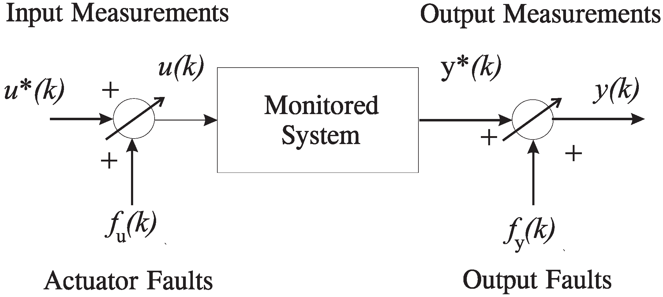
It is assumed that the monitored system is described as represented in
Figure 1. The prediction (or estimation error)
in fault-free conditions represents the model-reality mismatch, which accounts for process noise, parameter variations, disturbance and uncertainty.
Figure 1.
The monitored system.
Figure 1.
The monitored system.
The relations of Equation (
11) describe the realistic situation where the variables
and
are measured by means of sensors affected by both measurement noise and faults.
Neglecting the sensor dynamics, faults acting on the measured input and output signals
and
are modeled as:
where
and
represent additive signals assuming values different from zero only in the presence of faults.
There are different approaches to generate the residuals for fault diagnosis; see, e.g., [
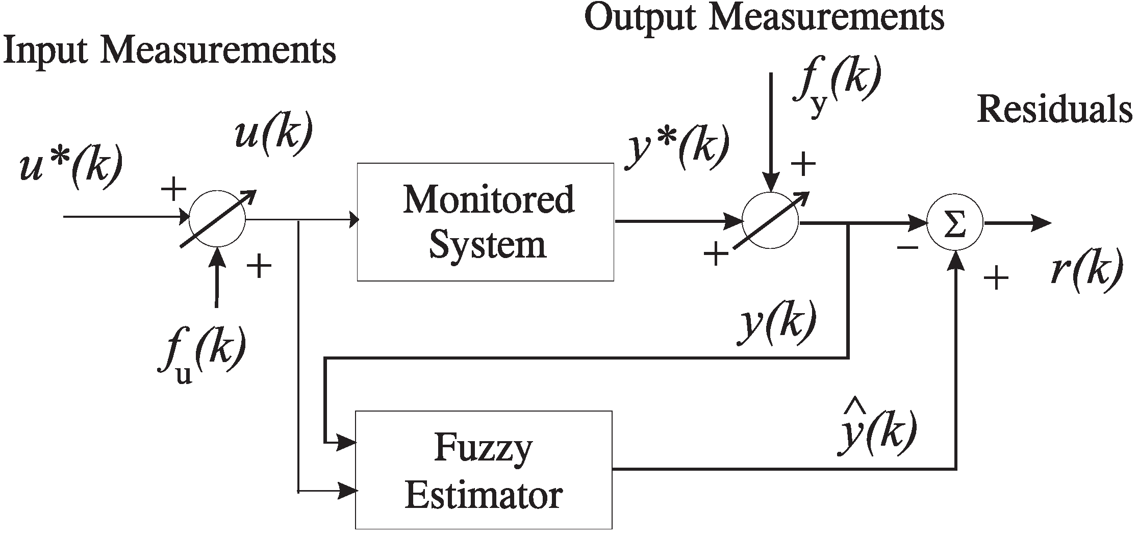
12]. In this work, the TS models are used as residual generators for the wind turbine system.
Figure 2 shows that the residuals are generated by the comparison of the measured
and the estimated outputs:
:
Figure 2.
The residual generation scheme.
Figure 2.
The residual generation scheme.
The symptom evaluation refers to a logic device that processes the redundant signals generated by the first block, in order to detect when a fault occurs and to univocally identify the unreliable actuator or sensor.
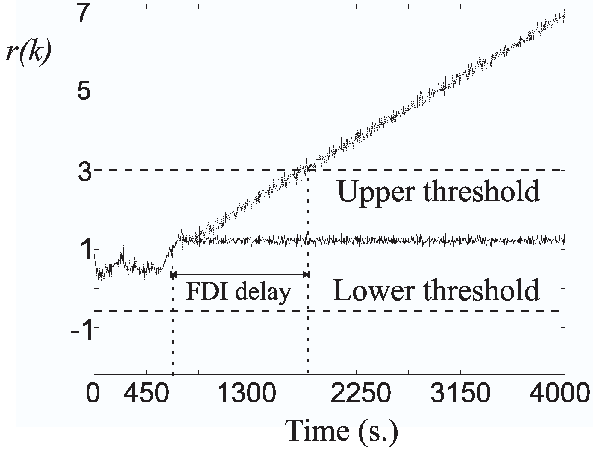
The fault detection task is performed here by using a simple thresholding logic, even if different strategies are available; see e.g., [
12]. It is worth noting that the faults described in
Section 2.1 may not be immediately detected, since the delay in the corresponding alarm normally depends on the fault mode. This situation is shown in
Figure 3, where suitable fault detection thresholds are fixed according to Equation (
15):
In practice, the residual signal is represented by the random variable
, whose sample mean value and variance values are estimated as follows:
and
are the values for the sample mean and variance of the fault-free residual, respectively.
N is the number of samples of
. The values of
and
depend on the signal
statistics, usually unknown.
In order to separate normal from faulty behavior, the tolerance parameter
δ (normally
) is selected and properly tuned. Hence, the proper choice of this parameter
δ leads to a good trade-off between the maximization of the fault detection probability and the minimization of the false alarm rate. This parameter
δ could be fixed with empirical rules or, once the values of
and
are estimated from the
signal, using the three-sigma rule. On the other hand, less conservative results are obtained with a procedure that determines via extensive simulations the optimal
δ minimizing the false alarm rate and maximizing the detection/isolation probability. This issue will be addressed in
Section 5.
Figure 3.
Detection thresholds and fault detection and isolation (FDI) delay for incipient faults.
Figure 3.
Detection thresholds and fault detection and isolation (FDI) delay for incipient faults.
Moreover, as shown in
Figure 3, if a detection delay is tolerable, which depends on the fault severity, the amplitude of the detectable/isolable fault is lower.
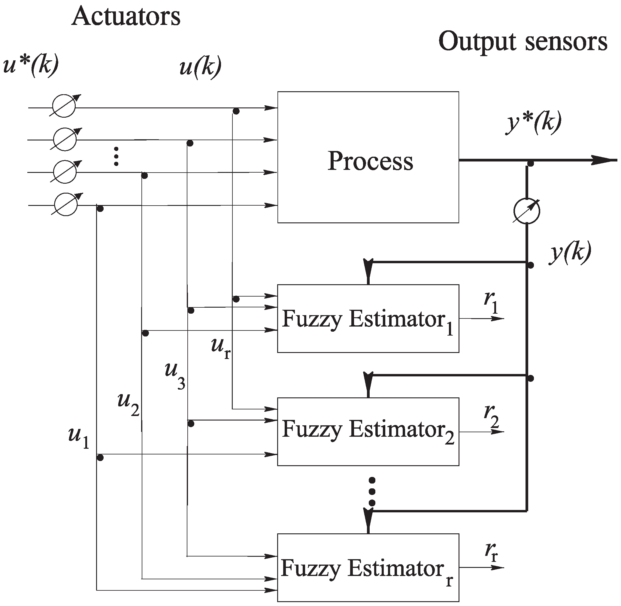
Finally, regarding the fault isolation problem, a generalized observer scheme (GOS) is exploited [
12]. In particular, as shown in
Section 2.1, since different faults
or
can affect the input or output measurements, to uniquely isolate a fault
concerning one of the inputs, under the assumption that the outputs are fault-free, a bank of estimators in the form of Equation (
5) is used, as shown in
Figure 4.
Figure 4.
Fuzzy estimator scheme for actuator fault isolation.
Figure 4.
Fuzzy estimator scheme for actuator fault isolation.
The number of these estimators is equal to the number of the faults
that have to be diagnosed. The
i-th fuzzy estimator is driven by all but the
i-th input (or even more inputs, if required) and all outputs of the system and generates a residual function, which is sensitive to all but the
i-th input fault
(or even more inputs, if necessary). The derivation of these fuzzy estimators follows the procedure described in
Section 3. In particular, when the fuzzy estimator insensitive to the
i-th input has to be designed, the output
and all but the
i-th inputs
are exploited for the identification process.
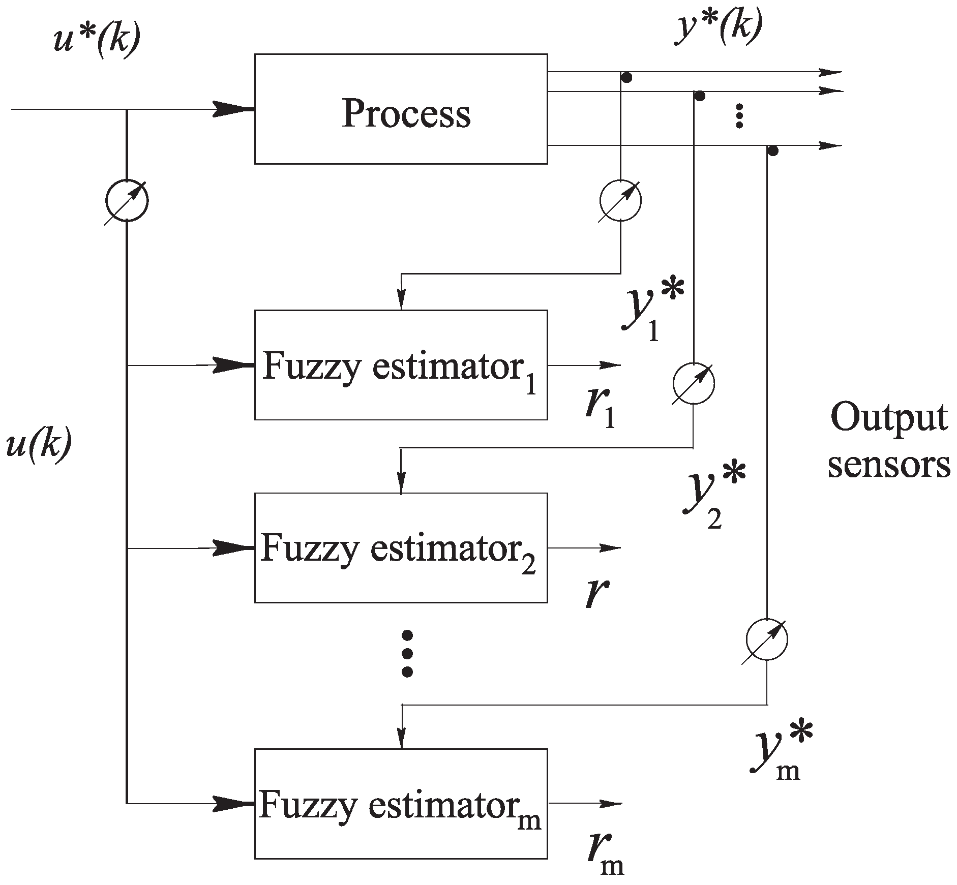
On the other hand, to uniquely isolate a fault
concerning one of the system outputs, under the hypothesis that inputs are fault-free, a bank of estimators is used again, according to
Figure 5.
This observer configuration represents the dedicated observer scheme (DOS) described in [
12]. The number of these estimators is equal to the number of faults
that have to be diagnosed, and each device is driven by a single output and all of the inputs of the system. In this case, a fault on the
i-th output affects only the residual function of the output observer or filter driven by the
i-th output.
In order to summarize the isolation capabilities of the schemes presented,
Table 4 shows the ‘fault signatures’ for the case of single fault occurrence. Note that in
Table 4, the residual
(
) coincides with the signal
of
Figure 4. On the other hand,
(
) represents the residual
of
Figure 5 for output fault isolation.
Figure 5.
Fuzzy estimators for sensor fault isolation.
Figure 5.
Fuzzy estimators for sensor fault isolation.
Table 4.
Fault signatures.
Table 4.
Fault signatures.
| | | | … | | | | … | |
| 0 | 1 | … | 1 | 1 | 1 | … | 1 |
| 1 | 0 | … | 1 | 1 | 1 | … | 1 |
| ⋮ | ⋮ | ⋮ | ⋮ | ⋮ | ⋮ | ⋮ | ⋮ | ⋮ |
| 1 | 1 | … | 0 | 1 | 1 | … | 1 |
| 1 | 1 | … | 1 | 1 | 0 | … | 0 |
| 1 | 1 | … | 1 | 0 | 1 | … | 0 |
| ⋮ | ⋮ | ⋮ | ⋮ | ⋮ | ⋮ | ⋮ | ⋮ | ⋮ |
| 1 | 1 | … | 1 | 0 | 0 | … | 1 |
The residuals affected by input and output faults are described by an entry ‘1’ in the corresponding table entry, while an entry ‘0’ means that the input or output fault does not affect the corresponding residual.
Note how multiple output faults can be isolated, since a fault on the i-th output signal affects only the residual function of the output estimator driven by the i-th output, but all of the residual functions . On the other hand, multiple faults on the inputs cannot be isolated, since, in general, all residual functions are sensitive to faults regarding different inputs.
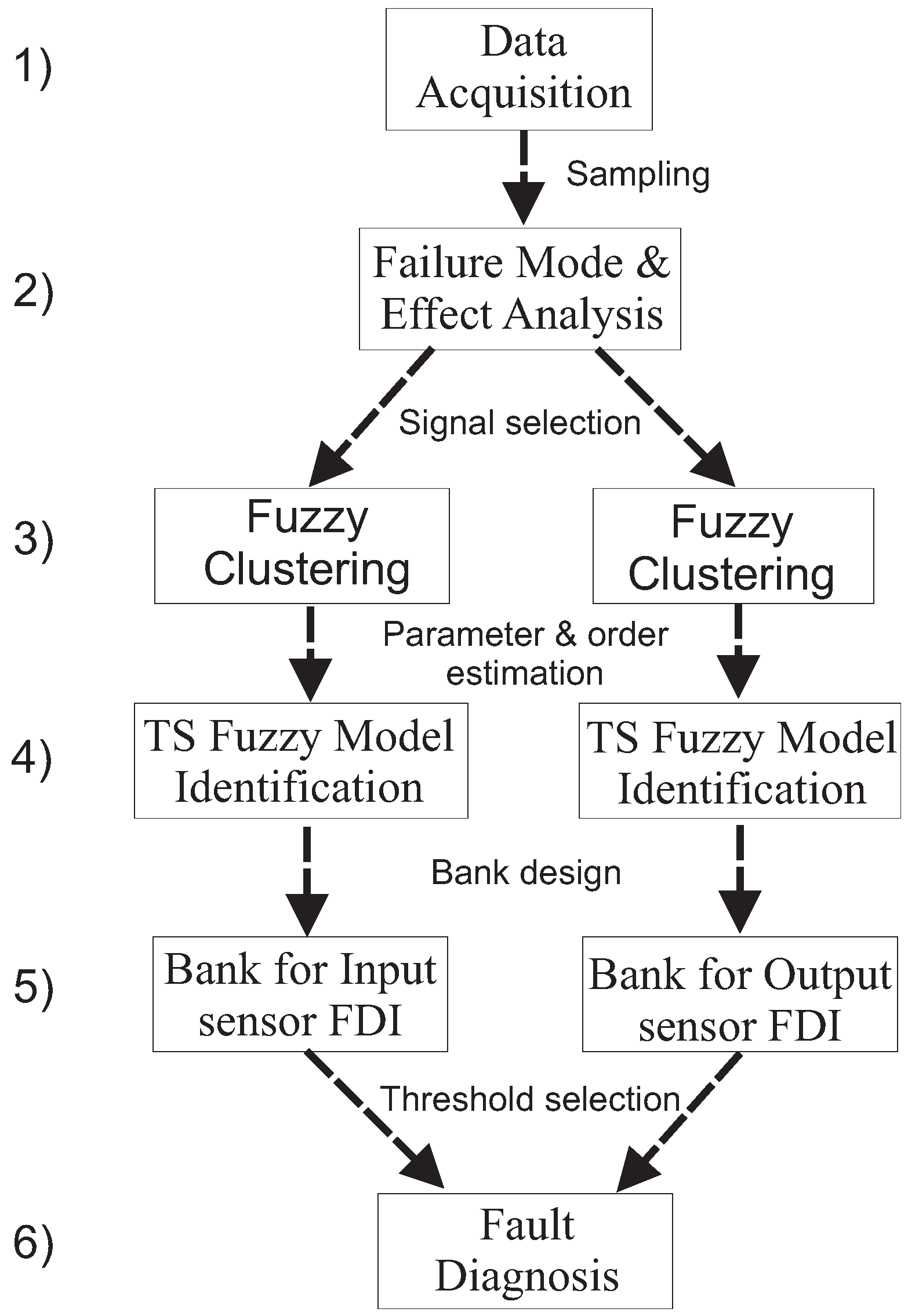
Finally, in order to summarize the complete procedure, the different design phases are summarized in
Figure 6.
Once the data have been collected and sampled from the wind turbine (Step 1), the FMEA recalled in
Section 2.1 is applied. This procedure suggests how to select the measured signals
and
(Step 2) in order to build the fuzzy estimator banks (Step 5) described in
Figure 4 and
Figure 5. The different fuzzy estimator models have the form of Equation (
5) derived using the fuzzy clustering (Step 3) recalled in
Section 3.1, followed by the structure identification (Step 4) in
Section 3.2. In this way, by means of the threshold test logic of Equation (
15), the fault diagnosis is achieved (Step 6).
Figure 6.
Sketch of the complete design procedure.
Figure 6.
Sketch of the complete design procedure.
5. Simulation Results
The proposed FDI methodology was applied to a sequence of data samples and acquired with a sampling rate of 100 Hz. from the wind turbine benchmark.
According to
Section 3 and
Section 4, the Gustafson–Kessel (GK) clustering method with
clusters and a number of shifts
was used for the identification of the fuzzy estimator banks of
Section 4. These optimal parameters
and
were obtained as described in [
16,
17]. After clustering, the parameters
and
, with
, were estimated using the identification method presented in
Section 3. Moreover, the membership degrees
required by the fuzzy estimators of Equation (
5) have been modeled as Gaussian functions.
As shown in
Figure 4 and
Figure 5, the reconstructed output
for the FDI task has been generated by a bank of five multiple-input single-output (MISO) predictors of Equation (
5). According to
Table 2 and
Figure 4, this scheme allows the diagnosis of Fault
, Fault
, Fault
, Fault
and Fault
. On the other hand, with reference again to
Table 2 and
Figure 5, a bank of four output fuzzy estimators for
allows the diagnosis of Fault
, Fault
, Fault
and Fault
.
For each fault case, by following the FMEA procedure described in
Section 2.1 and
Table 2, the input and output measurements used for the design of the estimator banks were reported in
Table 5.
The approximation capabilities of the fuzzy residual generators can be expressed in fault-free conditions in terms of the so-called variance accounted for (VAF) index [
15]. In particular, the VAF values for all identified MISO estimators were always bigger than 99%. Hence, the multiple model scheme seems to approximate the process outputs quite accurately. Note, in fact, that, as described in [
16,
17], with the choice of parameters
and
, the fuzzy predictors led to the minimization of the reconstruction errors,
i.e., the difference between the measured and predicted outputs.
Table 5.
Inputs and outputs for the fuzzy residual generator design.
Table 5.
Inputs and outputs for the fuzzy residual generator design.
| Fault | Inputs | Output |
|---|
| 1 | | |
| 2 | | |
| 3 | | |
| 4 | | |
| 5 | | |
| 6 | | |
| 7 | | |
| 8 | | |
| 9 | | |
The rationale of using TS fuzzy models was highlighted in
Section 3, whilst their efficacy is analyzed in the following.
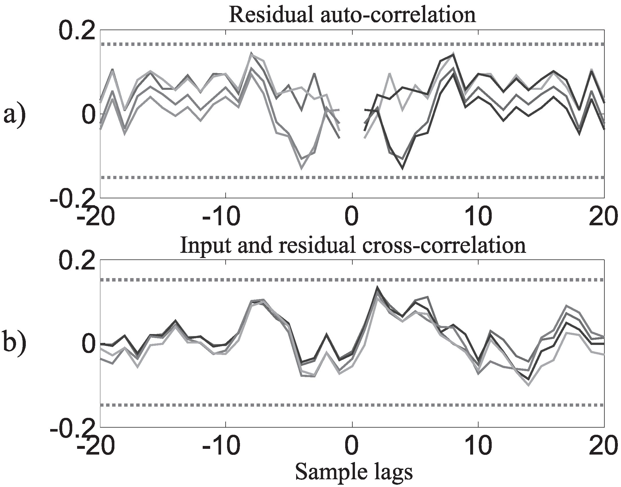
Figure 7 reports the results of the correlation analysis on the input variables. In fact, in fault-free conditions, the residuals
associated with the data of each cluster (
) and the identified affine models should be ideally white and independent of the inputs
. This situation guarantees that the estimators approximate correctly the measurements
in each cluster.
Figure 7.
Residual auto– and cross–correlation examples ().
Figure 7.
Residual auto– and cross–correlation examples ().
Figure 7 shows the estimator residuals
in fault-free conditions for each cluster (
), thus highlighting their whiteness and independence. In particular (1) the auto-correlation function of
and (2) the cross-correlation function between
and
are displayed for 20 lags. For these variables, the 99% confidence intervals are also depicted as dotted lines, thus showing that
is white and independent of
for each cluster. These results prove experimentally the validity of the TS models proposed in this study.
It is worth noting that the nonlinear benchmark originally developed in [
25] was modified by the authors in order to vary the statistical properties of the signals used for modeling process parameter uncertainty and measurement errors. Under this assumption,
Table 6 reports the nominal values of the considered wind turbine model parameters with respect to their simulated uncertainty. In this way, a Monte Carlo analysis can be performed for assessing the reliability and the robustness of the considered FDI scheme by modeling the model variables as Gaussian stochastic processes, with zero-mean and standard deviations corresponding to realistic minimal and maximal error values of
Table 6.
Table 6.
Realistic wind turbine uncertainty.
Table 6.
Realistic wind turbine uncertainty.
| Variable | Nominal Value | Min Error | Max Error |
|---|
| ρ | kg/m | ±0.1% | ±20% |
| J | kg/m | ±0.1% | ±30% |
| | ±0.1% | ±50% |
| u | | ±0.1% | ±20% |
| y | | ±0.1% | ±20% |
It is also assumed that the input-output signals
u and
y and the power coefficient map
entries were affected by errors, expressed as percent standard deviations of the corresponding nominal values
,
and
, also reported in
Table 6. Therefore, for the performance evaluation of the FDI methodologies, a sufficient number of Monte Carlo runs was performed.
Note that
Table 6 describes the uncertain parameters that have been simulated in order to analyze the reliability and the robustness features of the proposed approach with respect to parameter variations. In fact, the approach was proposed here also for removing the effect of the uncertain wind term
and not for handling the parameter variations summarized in
Table 6.
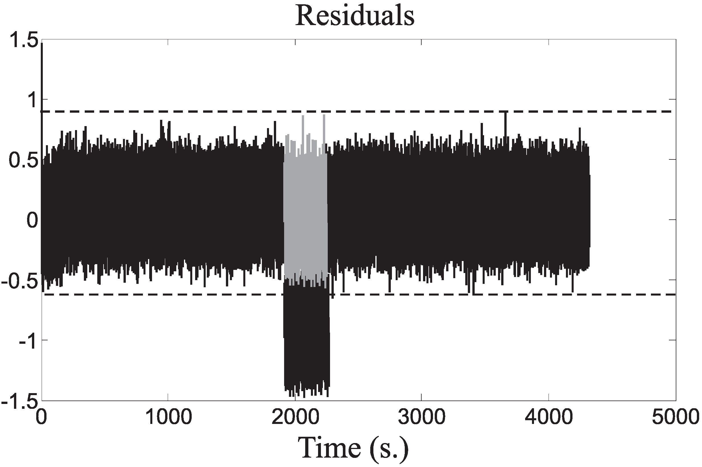
The simulations of different fault cases have been reported for highlighting the most important features of the proposed approach. In particular, the first example was obtained by considering the fault Case 1, commencing at the instant
s, and active for 100 s. The considered fault
causes alteration of the signals
and
and, therefore, of the residuals
given by the model of Equation (
5). These residuals indicate the fault occurrence according to the logic of Equation (
15), whether their values are lower or higher than the thresholds fixed in fault-free conditions.
Figure 8 represents the fault-free (grey continuous line) and the faulty (black dashed line) residuals
.
The fault detection thresholds of Equation (
15) are represented as dotted constant lines in
Figure 8. Their values were properly settled, as described in
Section 5.2, in order to minimize the false alarm and missed fault rates, while maximizing the correct detection and isolation rates. In these conditions, the fault is correctly detected and isolated when the corresponding residual signals exceed the thresholds, as indicated in
Figure 8.
Figure 8.
Residuals for the fault Case 1.
Figure 8.
Residuals for the fault Case 1.
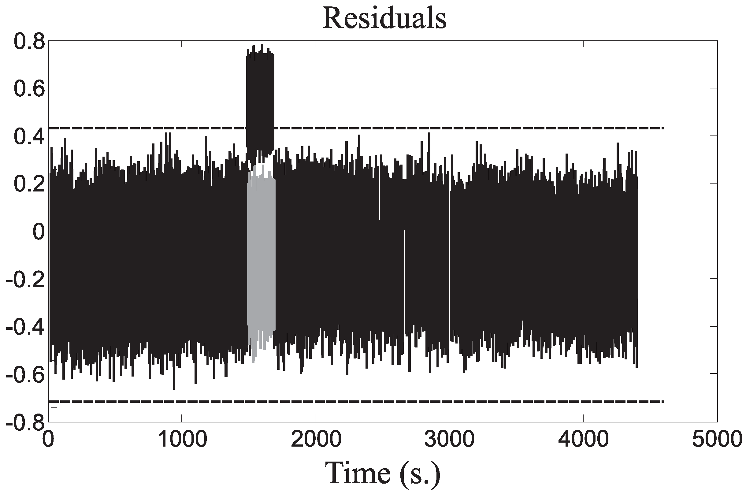
The second example depicted in
Figure 9 represents the fault-free (grey continuous line) and the faulty (black dashed line) residuals
related to the fault case 4,
i.e.,
. It commences at the instant
s, and it is active for 100 s. The fault detection thresholds, represented as dotted constant lines in
Figure 9, were optimally fixed, as in the previous case.
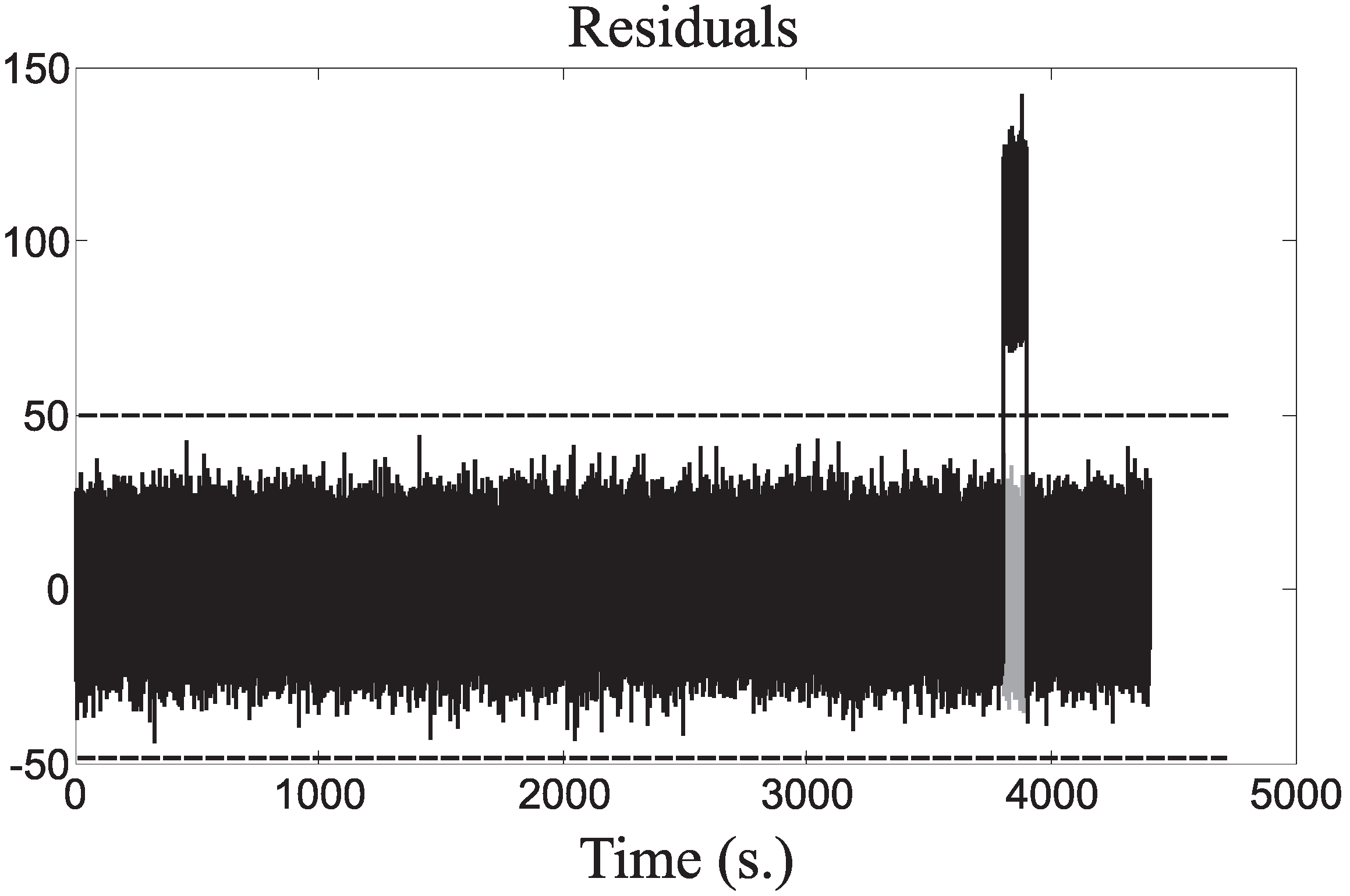
The third example was obtained by considering the fault Case 8,
i.e.,
, which is active between 3800 s and 3900 s.
Figure 10 represents the fault-free (grey continuous line) and the faulty (black dashed line) residuals
.
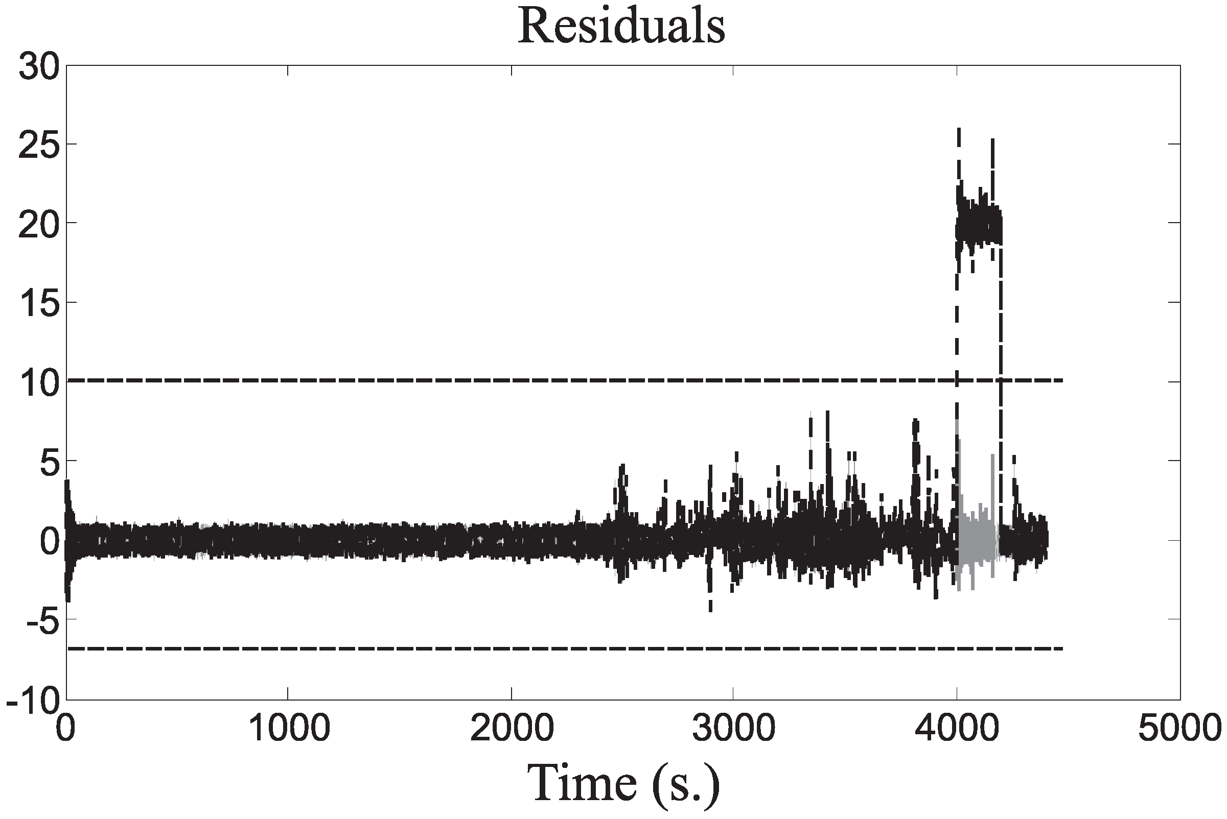
Finally,
Figure 11 depicts the fault-free (grey continuous line) and the faulty (black dashed line) residuals
related to the fault Case 9,
i.e.,
, active between 4000 s and 4200 s. Again, the FDI thresholds represented in
Figure 11 were optimally fixed, as in the previous case.
Figure 9.
Residuals for the fault Case 4.
Figure 9.
Residuals for the fault Case 4.
Figure 10.
Residuals for the fault Case 8.
Figure 10.
Residuals for the fault Case 8.
Figure 11.
Residuals for the fault Case 9.
Figure 11.
Residuals for the fault Case 9.
5.1. Comparative Studies
This section provides some comparative results with respect to different FDI schemes.
The first alternative approach considered here uses a support vector machine based on a Gaussian kernel (GKSV) developed in [
8]. The scheme defines a vector of features for each fault, which contains relevant signals obtained directly from measurements, filtered measurements or their combinations. These vectors are subsequently projected onto the kernel of the support vector machine (SVM), which provides suitable residuals for all of the defined faults. Different kernels have been tested, and it was found that Gaussian kernel with different variance values can be used for all faults. Data with and without faults were used for learning the model for the FDI of the specific faults.
The second scheme consists of an estimation-based (EB) solution shown in [
10]. In particular, a fault detection estimator is designed to detect a fault, and an additional bank of estimators is derived to isolate them. The method was designed on the basis of a system linear model and used fixed thresholds, as in Equation (
15). Each estimator for fault isolation was computed on the basis of the particular fault scenario under consideration.
The third method relying on up-down counters (UDCs) was addressed in [
11]. These tools, borrowed from the aerospace framework, were exploited in the decision logic applied to the FDI residuals. These residuals were obtained using both physical and analytical redundancy schemes, such as parity equations from redundant sensors and Kalman filters. This approach is different from the straightforward thresholding of Equation (
15). In fact, the decision to declare the fault occurrence involves discrete-time dynamics and is not simply a function of the residual current value.
The fourth approach combines observer and Kalman filter (COK) methods [
7]. It relies on an observer used as a residual generator for diagnosing the faults of the drive-train, in which the wind speed is considered a disturbance. This diagnosis observer was designed to decouple the disturbance and simultaneously achieve optimal residual generation in a statistical sense. For the other two subsystems of the wind turbine, a Kalman filter-based approach was applied. The residual evaluation task used a generalized likelihood ratio test, and cumulative variance indices were applied. For fault isolation purpose, a bank of residual generators was exploited. Sensor and system faults were thus isolated via a decision table.
The fifth method relies on the general fault model (GFM) scheme, which is a method of automatic design [
9]. The FDI strategy consists of three main steps. In the first step, a large set of potential residual generators was designed. In the second step, the most suitable residual generators to be included in the final FDI system were selected. In the third step, tests for the selected set of residual generators were performed, which were based on comparisons of the estimated probability distributions of the residuals, evaluated with fault-free and faulty data.
For performance evaluation and comparison of the considered FDI schemes, some indices have been used. They were presented in [
26] and here evaluated on
Monte Carlo runs. These indices are defined as:
False Alarm Rate (): the number of wrongly detected faults divided by total fault cases;
Missed Fault Rate (): for each fault, the total number of undetected faults, divided by the total number of times that the fault case occurs;
True Detection/Isolation Rate (): for a particular fault case, the number of times it is correctly detected/isolated, divided by total number of times that the fault case occurs;
Mean Detection/Isolation Delay (): for a particular fault case, the average detection/isolation delay time.
These criteria are computed for each fault case and for each FDI scheme.
Table 7 summarizes also the results obtained by considering the fuzzy predictors as residual generators (FPRG) and with an optimal choice of the threshold parameter
δ in Equation (
15) that leads to achieving optimal results.
Several comments can be drawn here. GKSV is able to detect and isolate Faults 1, 2, 3, 4, 5 and 8 and some of them with delays bigger than 25 s. For these diagnosable faults, the average detection rate is bigger than 65%, with missed fault and false alarm rates lower than 35%. Moreover, in general, this scheme showed robustness with respect to the working point changes of the wind turbine, but effective only on sensor faults. EB manages the faults quite quickly, apart from Fault 9. For the detectable faults, the detection rate is bigger than 66%, with missed fault and false alarm rates lower than 33%. The diagnosis delays for Faults 2, 6 and 7 can be bigger than 11 s. In particular, for Faults 2 and 9, false alarms can occur. UDC detects and isolates almost all faults, apart from Fault 9, with delay times lower than 69 s. However, false alarm rates bigger than 12% are measured for Faults 2, 3, 4, 5, 6, 7 and 8. In the same way, COK is able to detect and isolate faults, apart from 9, and in general, with a delay time bigger that 10 s. False alarm and missed fault rates bigger that 10% can also occur. The same considerations holds for the GFM solution. The detection delay times can be bigger than 9 s, with false alarm and missed fault rates bigger that 12%. Regarding the proposed FPRG method, it seems to work relatively better than the others, even if optimization stages are required, for example, for the optimal FDI threshold selection. For this method, in general, also for Fault 9, the detection rates are bigger than 83%, with false alarm and missed fault rates lower than 14%. The issue of the optimal threshold selection will be analyzed in
Section 5.2. Note finally that the simulator used in this study was modified by the authors, and the working conditions can be slightly different from the ones shown in [
6].
5.2. Robustness Evaluation
This section reports further experimental results regarding the performance optimization of the developed FDI scheme with respect to modeling errors and measurement uncertainty. In particular, the simulation of different fault-free and faulty data sequences has been performed by exploiting again the wind turbine simulator and the Monte Carlo method. In fact, the Monte Carlo tool is useful at this stage, since the efficacy of the FDI module depends on both the model approximation and the measurement errors.
Therefore, the indices defined above have been evaluated for each fault case. In particular,
Table 8 summarizes the results obtained by considering the fuzzy predictors as residual generators and with a choice of the parameter
δ of Equation (
15) that leads to optimal performances.
Table 8 shows that the proper selection of the threshold levels of Equation (
15) depending on
δ allows one to achieve false alarm and missed fault rates of less than 13% and detection/isolation rates larger than 83%, with minimal detection/isolation delay times. The results demonstrate also that Monte Carlo analysis is an effective tool for experimentally tuning and testing the suggested FDI method. In the presence of uncertainty and modeling errors, this latter simulation technique seems to facilitate the assessment of the reliability of the developed FDI methods for application to real test cases.


