Pollutant Emission Validation of a Heavy-Duty Gas Turbine Burner by CFD Modeling

Department of Astronautics, Electrical and Energy Engineering, University of Rome, "Sapienza", via Eudossiana 18, Rome 00184, Italy
Machines 2013, 1(3), 81-97; https://doi.org/10.3390/machines1030081
Submission received: 17 June 2013
/
Revised: 27 August 2013
/
Accepted: 27 September 2013
/
Published: 16 October 2013
(This article belongs to the Special Issue Advances in Control Engineering)
Abstract
:3D numerical combustion simulation in a can burner fed with methane was carried out in order to evaluate pollutant emissions and the temperature field. As a case study, the General Electric Frame 6001B system was considered. The numerical investigation has been performed using the CFD code named ACE+ Multiphysics (by Esi-Group). The model was validated against the experimental data provided by Cofely GDF SUEZ and related to a real power plant. To completely investigate the stability of the model, several operating conditions were taken into account, at both nominal and partial load. In particular, the influence on emissions of some important parameters, such as air temperature at compressor intake and steam to fuel mass ratio, have been evaluated. The flamelet model and Zeldovich’s mechanism were employed for combustion modeling and NOx emissions, respectively. With regard to CO estimation, an innovative approach was used to compute the Rizk and Mongia relationship through a user-defined function. Numerical results showed good agreement with experimental data in most of the cases: the best results were obtained in the NOx prediction, while unburned fuel was slightly overestimated.
1. Introduction
In recent decades, stationary gas turbines have become firmly established as prime movers in the gas and oil industry, acquiring new ranges of application in many areas of utility power generation and, in particular, in combined cycle plants [1]. These developments have been accompanied by a continuous increase in pressure ratio, and furthermore, many practices were developed to reduce pollutant emissions and their impact on health and the environment, keeping a high combustion efficiency in a wide range of operating conditions. In general, the combustion efficiency and the performance of a burner depend on the quality of the fuel-air mixture [2]. In systems where the fuel is directly injected into the combustion chamber, it is necessary that the fuel is mixed into the air over a time interval comparable with the burning rate of the mixture. In this system, the Reynolds number characterizes the intensity of the turbulent mixing, while the Damköhler number (Da) characterizes the rate of the mixing against the rate of the chemical reactions. Specifically, this number represents the quotient of a characteristic time scale of turbulence/mixing and a characteristic time scale of chemical reactions: larger Da corresponds to faster reactions [3]. This phenomenon depends on many parameters that can be classified into two distinct groups: those related to the injection system and those related to the environment in which the injected gas evolves. From a numerical point of view, a CFD investigation of the mixture formation processes can be carried out only by making use of meshes whose refinement is able to accurately describe fuel mixing and its dispersion within the region near the injector and the primary zone [4].
In the present article, the numerical study was set with reference to operating conditions of one of the ten burners of the FRAME 6B General Electric gas turbine machine, having the nominal electric power of 40 MWe. In particular, the simulations referring to both nominal and partial load conditions were investigated, focusing attention on the thermal field and pollutant emissions in order to firstly validate the numerical model through experimental data. Secondly, the model was used to obtain regression laws to predict pollutant emissions out of the simulated ranges or to improve the employed correlations. This information is important, since it represents a starting point of a more complex study for the evaluation of the power plant conversion to bio-liquid. The first step is thus the construction of a numerical model to reproduce the actual configuration and its operating conditions. The experimental data were provided by Cofely GDF SUEZ and related to the combined cogenerative power plant located in Nera Montoro (Narni, Italy), whose characteristics will be described in the following paragraphs.
2. The Power Plant
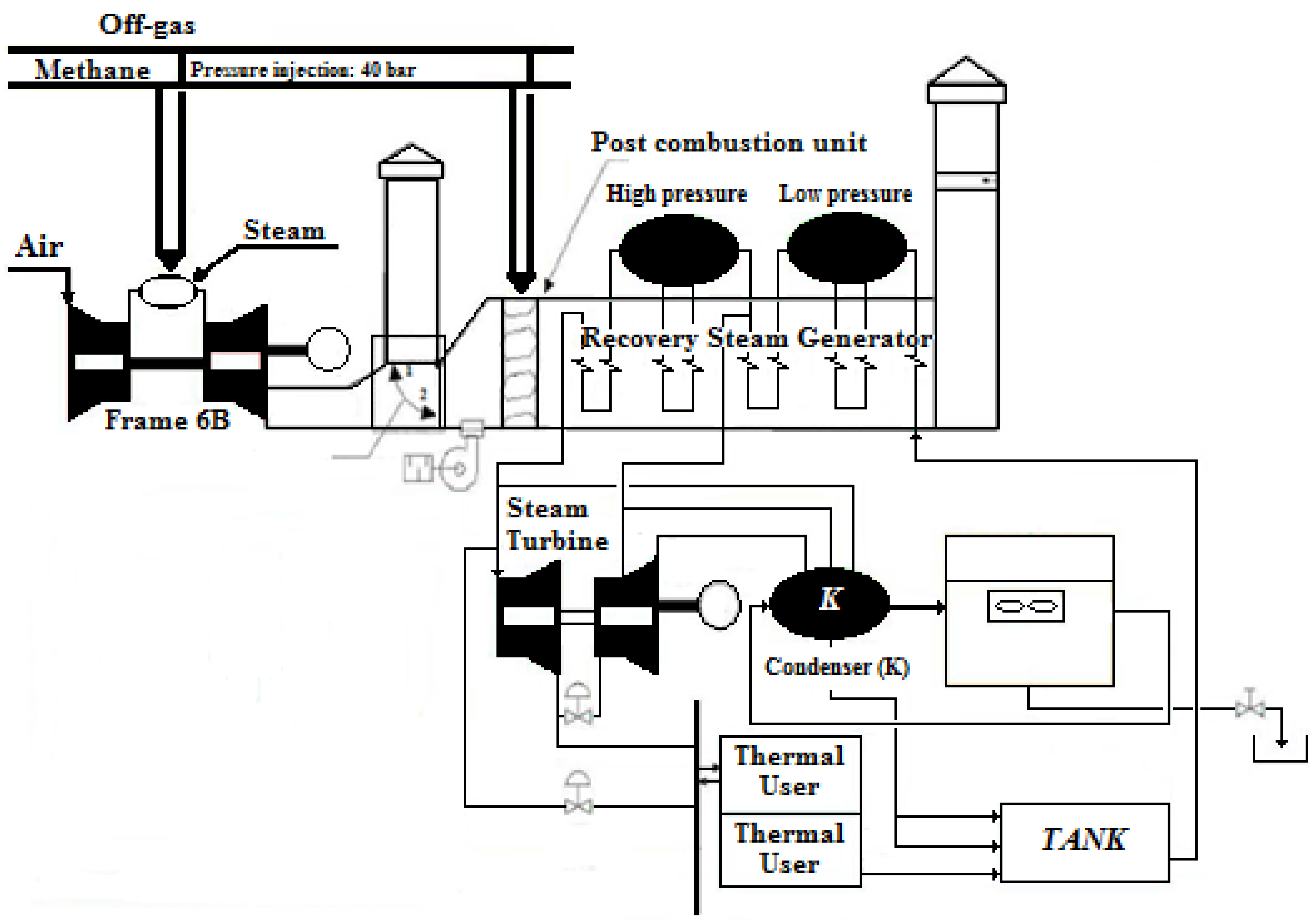
The gas turbine we studied is installed within a combined cycle power plant whose steam turbine has a nominal electric power of 12 MWe (Figure 1). To reduce NOx pollutant emissions, bled steam from the high pressure turbine is injected within the combustion chambers of the gas turbine. The main operating parameters of the gas turbine and steam injection system are reported in Table 1, and they refer to the nominal operating conditions. The electrical energy is introduced into the grid and remunerated through the CIP6 feed-in tariff law; the steam is sold to the thermal users connected with the power plant.
The power plant can be fed with both methane and off-gas, the latter produced by one of the thermal users. Since the off-gas contribution is minimal, our studies have focused on methane. The most important parameters regarding the fuel injection system are listed in Table 2.
Figure 1.
Power plant schematization.


| Engine Type | Frame 6B (General Electric) |
|---|---|
| Air | |
| Compression ratio (β) | 11.8:1 |
| Temperature at the end of compression | 670 K |
| Mass flow rate (kg/s) | 139 kg/s |
| Engine speed (at nominal conditions) | 5,115 rpm |
| Steam | |
| Injection pressure | Variable (up to 40 bar) |
| Temperature | 620 K |
| Mass flow rate | Minimum: 0.208/Maximum: 0.445 kg/(s·can) |
| Nozzle hole diameter | 2 mm |
| Injector Type | Pressure swirl Atomizer |
|---|---|
| Injection pressure | 40:1 |
| Temperature | 350 K |
| Mass flow rate | 0.28 kg/s |
| Number of nozzles | 4 |
| Fuel to air ratio (FAR) | 0.019 |
| Fuel | Methane/off-gas |
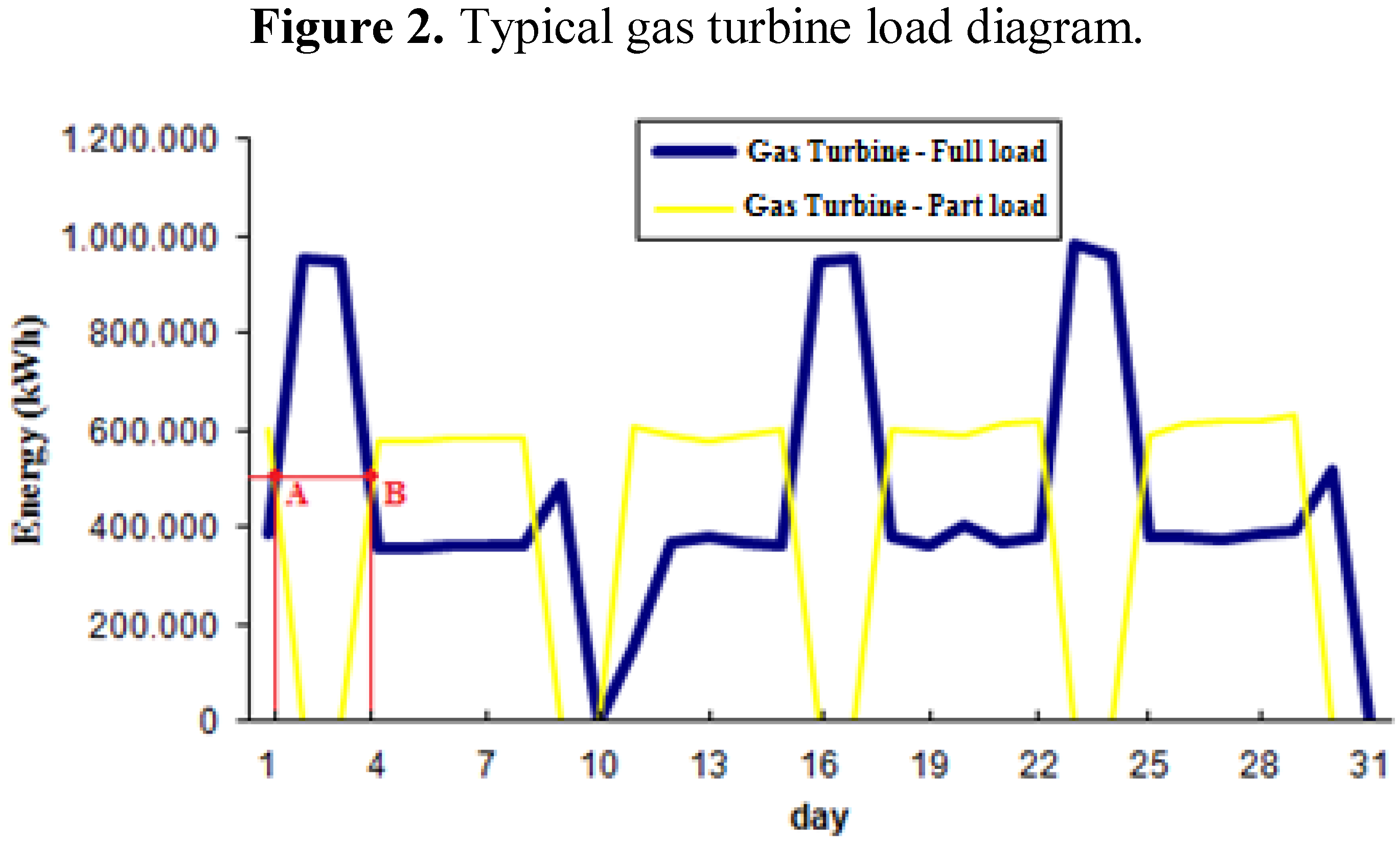
The steam can be produced by both the heat recovery generator and the post combustion unit: when the steam demand is at the maximum level, these two sections operate in parallel, with the gas turbine working at partial load. Figure 2 reports a typical load diagram for the gas turbine: the blue line represents the produced energy with the gas turbine working at nominal conditions and the yellow one, the energy produced at partial load. For example, during days 1 and 4, the gas turbine produced the same energy (about 500,000 kWh) working at full load and partial load.
Figure 2.
Typical gas turbine load diagram.

Considering the most frequent operating conditions of the plant, simulations for 75, 80, 90 and 100% of the nominal thermal power have been taken into account. Obviously, changes of the air conditions due to compressor regulation have been considered, too. The information about the pollutant emissions will be reported in the following paragraphs, where they will be compared with the numerical results.
3. Numerical Procedure
3.1. Burner Geometry and Grid Discretization
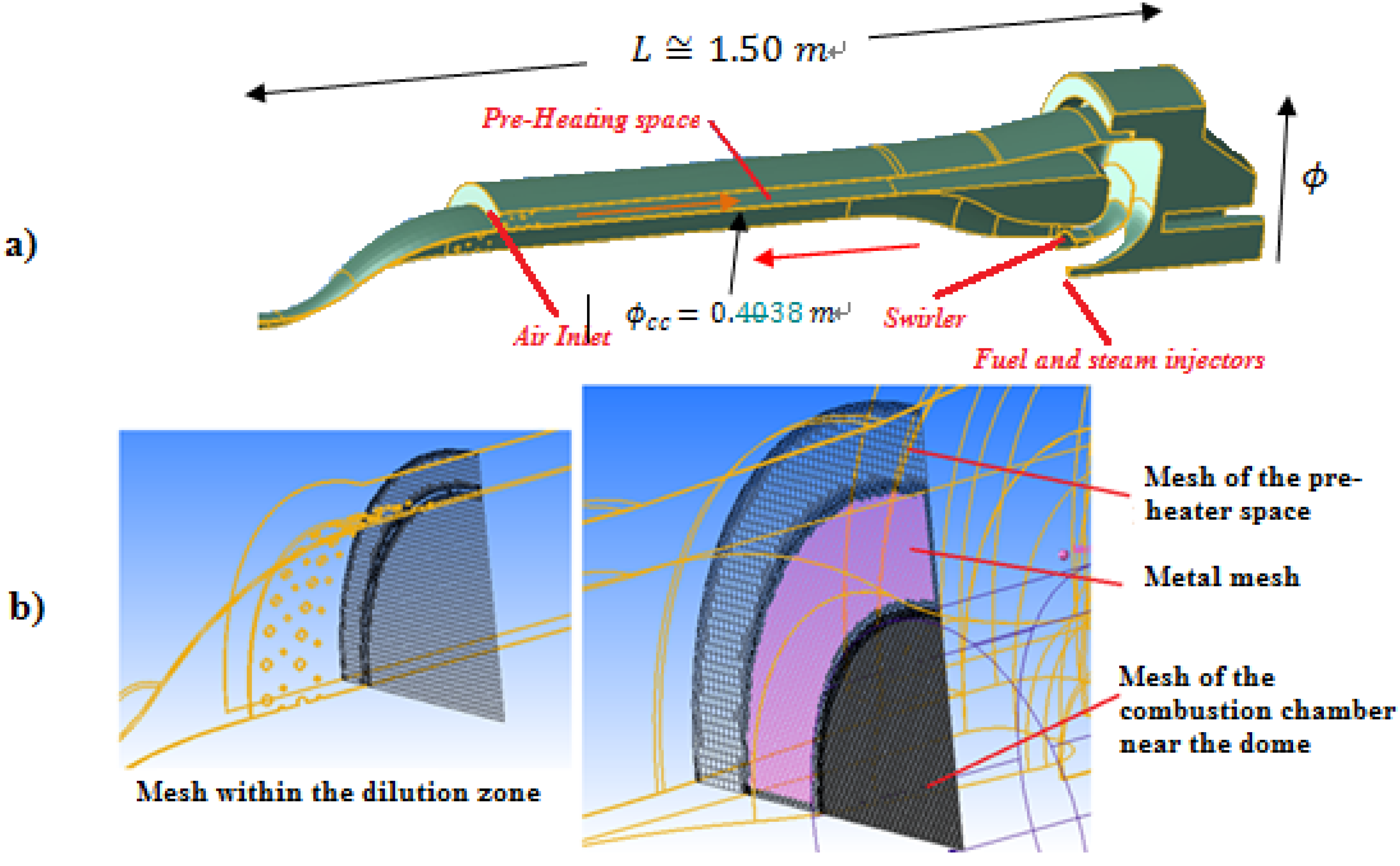
The FRAME 6B can is a reverse-flow combustor, i.e., the air coming from the compressor is passed inside a pre-heating space heading from the base towards the dome. This path allows the compressed air to be heated and to enter the combustion chamber with a higher temperature than that at the end of compression, thus increasing the combustion efficiency.
When the air arrives close to the dome, it is swirled and pushed into the primary combustion zone. The injectors of the fuel gas and of the steam are placed in the terminal part of the dome. The central part of the liner, where the combustion chemical reactions develop, is followed by a dilution zone: the holes on the walls of the liner have the dual function to dilute the exhaust gas flow and cool the walls of the combustion chamber. The total length of the burner and its maximum diameter are about 1.50 m and 0.56 m, respectively (Figure 3); the diameter of the combustion chamber is 0.38 m.
The computational mesh was created using the ACE+ Multiphysics tool. Because of the symmetry of the system and its components, the CFD calculations are performed on 90° sector meshes. Two different domains have been defined: the first is related to fluid volume, the second to the metal walls of the liner. This choice allows the pre-heating of the compressed air that occurs in the interspace to be described, solving concurrently fluid-dynamic and heat transfer equations. In both cases, unstructured meshes have been chosen. With regard to the fluid mesh, more dense discretizations have been located near the outlet sections of the fuel and steam injectors, where the speed of the jets takes on values on the order of hundreds of meters per second and within the primary and secondary zones. Table 3 summarizes the characteristics of the fluid grid in each region of the burner. The adopted resolution was found to give adequately grid independent results.
Figure 3.
(a) Main components of the burner (Computer Aided Drafting model); (b) and details of the mesh.
Figure 3.
(a) Main components of the burner (Computer Aided Drafting model); (b) and details of the mesh.
| Region | Characteristics |
|---|---|
| Pre-heater region | Cell type: hexahedral |
| Averaged cell resolution: ϕcc/210 | |
| Injectors region | Axial length: 5 cm |
| Cell type: hexahedral | |
| Averaged cell resolution: ϕcc/475 | |
| Combustion chamber: primary and secondary zones | Cell type: hexahedral |
| Averaged cell resolution: ϕcc/315 | |
| Combustion chamber: dilution zone | Cell type: hexahedral |
| Averaged cell resolution: ϕcc/210 | |
| Wall region | Two layer of tetrahedral cells |
| Total number of cells | 1.5 million cells |
Table 4 provides more details about mesh boundaries. In particular, the air mass flow rate at the inlet of the single burner (cf. Table 1) has been defined through the specification of the velocity and the temperature, so that the experimental data have been directly introduced into the numerical model. This choice allows these parameters to be easily changed to follow the different operating conditions of the burner; for example, at partial load conditions, the effect of the Inlet Guide Vane (IGV) on the flow has been modeled by changing the numerical value of the flow velocity. On the contrary, the turbulence intensity has not been modified during simulations (cf. Table 4).
| Boundary | Type | Value (at Nominal Condition) | Turbulence |
|---|---|---|---|
| Air inlet | Velocity inlet | 28 m/s (normal to boundary) | Turbulence intensity: 0.08 |
| Dissipation rate: 0.055 m (hydraulic diameter) | |||
| Gas outlet | Pressure outlet | 11.8 bar | Back flow kinetic energy: 0.01 m2/s2 |
| Dissipation rate: 0.135 m (hydraulic diameter) | |||
| Fuel inlet | Mass flow rate inlet | 0.07 kg/s (for the single nozzle) | Turbulence intensity: 0.12 |
| Dissipation rate: 0.001 m (hydraulic diameter) | |||
| Steam inlet | Mass flow rate inlet | 0.032 kg/s (for the single nozzle) | Turbulence intensity: 0.12 |
| Dissipation rate: 0.002 m (hydraulic diameter) |
3.2. The Turbulent Combustion Model
As to the turbulent closure, the k-ε approach with standard wall function has been used to model the turbulent effects. With regard to the combustion model, a chemistry with 35 species and 177 reactions was employed. This is a homemade chemistry derived from the detailed mechanism, GRIMech 3.0 [5] using the Open Source software, Kintecus, and, specifically, its tool, Atropos [6]. The Atropos software addition to Kintecus allows one to accurately reduce species and reactions out of larger systems that have no bearing on the results. This is realized through a sophisticated principle component analysis (PCA) on the basis of the normalized sensitivity coefficients (NSC) files outputted by Kintecus. The employed mechanisms result in being not so large as to be integrated within a multi-dimensional CFD code for the computing of laminar flamelets.
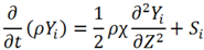
The flamelet model, used in the non-premixed combustion approach to account for chemical non-equilibrium, regards the turbulent flame as an ensemble of thin, locally one-dimensional flamelet structures. In this work, three flamelets with strain rate χ equal to 0.01, 0.1, one and 57 flamelets with initial strain rate χ0 = 2 and Δχ = 1 have been generated to characterize combustion. Using flamelets, species mass fraction, temperature, as well as the chemical reactions can be computed as a function of the mixture fraction (Z) and the strain rate (χ) only. After translation of the flamelet equations from a physical space to a mixture fraction space, a set of simplified equations can be re-written in the mixture fraction space, including equations for the species mass fraction (Equation (1)) and “solved for temperature” energy (Equation (2)) [7,8]:
![Machines 01 00081 i001]()
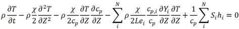
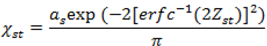
![Machines 01 00081 i002]() where Yi, T, ρ, Z, Si and hi represent the mass fraction, temperature, density, mixture fraction, reaction rate and enthalpy of the i-th species, respectively; cp,i and cp are the specific heat of the i-th species and the specific heat of the mixture. At the stoichiometric condition, the strain rate χ and the mixture fraction Z are related according to the following Equation (3):
where Yi, T, ρ, Z, Si and hi represent the mass fraction, temperature, density, mixture fraction, reaction rate and enthalpy of the i-th species, respectively; cp,i and cp are the specific heat of the i-th species and the specific heat of the mixture. At the stoichiometric condition, the strain rate χ and the mixture fraction Z are related according to the following Equation (3):
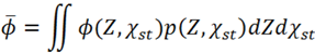
![Machines 01 00081 i003]() where as is a characteristic strain rate, Zst and χst are the mixture fraction and the strain rate at the stoichiometric condition, and erfc is the complementary error function. In the turbulent flame, both Z and χst are random variables with a joint probability density function (PDF). Therefore, the characteristic scalar (such as density, temperature and mass fraction) in the turbulent diffusion flame may be gained by laminar flamelet statistically:
where as is a characteristic strain rate, Zst and χst are the mixture fraction and the strain rate at the stoichiometric condition, and erfc is the complementary error function. In the turbulent flame, both Z and χst are random variables with a joint probability density function (PDF). Therefore, the characteristic scalar (such as density, temperature and mass fraction) in the turbulent diffusion flame may be gained by laminar flamelet statistically:
![Machines 01 00081 i004]()
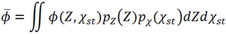
Assuming that Z and χst have independent distributions, the previous equation can be written as:
![Machines 01 00081 i005]()
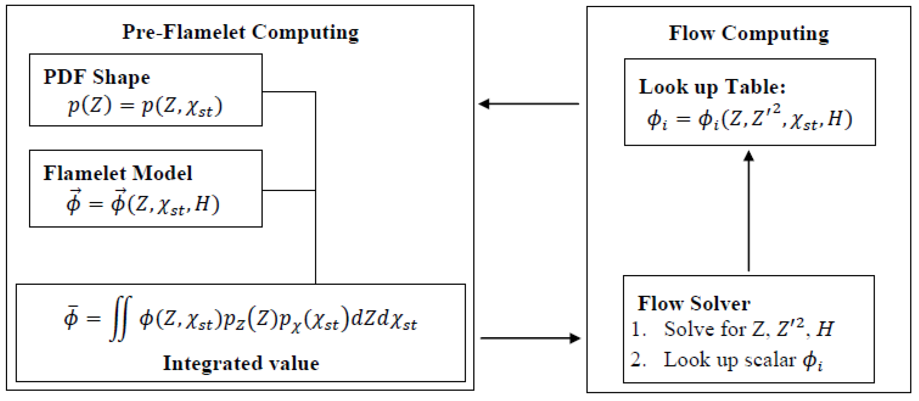
Equations (1) and (2) for species mass fraction and energy are solved simultaneously with the flow: the flamelet equations are advanced for a fractional time-step using properties computed from the fluid flow, and then, the latter is advanced for the same fractional time-step using properties from the flamelets (Figure 4). The flamelet time-step is computed through the volume-averaged scalar dissipation, pressure, fuel and oxidizer temperatures, which are passed from the flow solver to the flamelet solver.
Figure 4.
Flamelet model computing. PDF, probability density function.
3.3. The Pollutant Emission Models
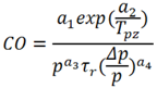
For the estimation of CO emission, an innovative approach has been used. The following semi-analytical correlation proposed by Rizk and Mongia has been implemented into a user-defined function (UDF) [9]:
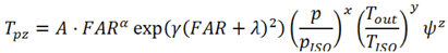
![Machines 01 00081 i006]() where the values of the constants are reported in the following Table 5 and the burner pressure loss, Δp, has been fixed to 4%. This equation allows carbon monoxide concentration to be related to important operating physical quantities, since there are two fundamental parameters in the previous equation: τr represents the residence time of the methane parcels within the combustion zone and Tpz, the averaged temperature in the primary zone. Using the software particle tracking, the methane parcels are followed until they have been completely consumed by combustion; an averaged value of the axial distance covered by parcels and their residence time are transferred to the UDF. According to [10], the temperature of the primary zone has been calculated as follows:
where the values of the constants are reported in the following Table 5 and the burner pressure loss, Δp, has been fixed to 4%. This equation allows carbon monoxide concentration to be related to important operating physical quantities, since there are two fundamental parameters in the previous equation: τr represents the residence time of the methane parcels within the combustion zone and Tpz, the averaged temperature in the primary zone. Using the software particle tracking, the methane parcels are followed until they have been completely consumed by combustion; an averaged value of the axial distance covered by parcels and their residence time are transferred to the UDF. According to [10], the temperature of the primary zone has been calculated as follows:
![Machines 01 00081 i007]() where:
where:
- -
- -
- -
- Tout is the averaged numerical temperature at the burner discharge;
- -
- ѱ the hydrogen to carbon atomic ratio, equal to four for methane.
Table 5.
Values of the constants for CO prediction [9].
| a1 | a2 | a3 | a4 |
|---|---|---|---|
| 66.48 ×10⁶ | 28.16 | 2.69 | 0.5 |
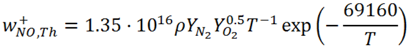
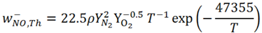
The extended Zeldovich’s mechanism has been taken into account to model reactions for thermal NOx formation:
![Machines 01 00081 i008]()

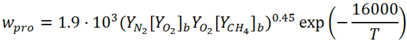
Prompt NO is caused by the presence of radicals in the flame zone; the following equation was adopted to compute its contribution [11]:
![Machines 01 00081 i011]() where the subscript, “b”, denotes the concentration of the species before the start of the combustion.
where the subscript, “b”, denotes the concentration of the species before the start of the combustion.
3.4. Heat Transfer Modeling for the Pre-Heating of the Air
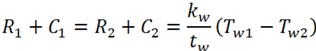
Heat transfer modeling involves the wall of the liner. The gas-side (Tw1) and the air-side (Tw2) wall temperatures of the liner can be computed using the following equilibrium equations, involving the gas-side and air-side radiation (R) and convection (C) contributes:
![Machines 01 00081 i012]() where kw and tw are the thermal conductivity and the thickness of the liner, respectively. As a simplifying assumption, the external radiation, R2, has been neglected, being quite small compared with the external convective heat transfer, C2. Thus, the remaining contributes are computed by the software as follows [11]:
where kw and tw are the thermal conductivity and the thickness of the liner, respectively. As a simplifying assumption, the external radiation, R2, has been neglected, being quite small compared with the external convective heat transfer, C2. Thus, the remaining contributes are computed by the software as follows [11]:
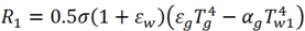
![Machines 01 00081 i013]()
![Machines 01 00081 i014]()
![Machines 01 00081 i015]() where σ is the Stefan-Boltzmann constant, εg and αg are the gas emissivity and absorptivity that are a function of the gas composition, 0.5 × (1 + εw) is the effective wall absorptivity, Tg and Tair are the local gas and air temperature and h1 and h2 are the gas-side and air-side heat transfer coefficients. The latter have been computed based on the local flow-field conditions, assuming a fully developed turbulent heat transfer within the annulus.
where σ is the Stefan-Boltzmann constant, εg and αg are the gas emissivity and absorptivity that are a function of the gas composition, 0.5 × (1 + εw) is the effective wall absorptivity, Tg and Tair are the local gas and air temperature and h1 and h2 are the gas-side and air-side heat transfer coefficients. The latter have been computed based on the local flow-field conditions, assuming a fully developed turbulent heat transfer within the annulus.
4. Results and Discussions
4.1. Comparison between Experimental and Numerical Results at 100% Load
A comparison of the results with experimental data can be carried out focusing attention only on the discharge temperature of the combustion chamber. The values reported in Table 6 refer to nominal conditions for the gas turbine and Standard conditions (ISO) for the environment and summarize the results that have been obtained in terms of pollutant emissions, too. Their concentration represent volume-weighted average values at the outlet section of the burner. NOx and CO formation can be estimated, but there is only one measured value; for further assessment of the prediction capability of the model, several simulations with different air temperatures at the inlet of the compressor were performed in order to carry out a sensitivity analysis.
| Firing Temperature | NOx Pollutant Emission | CO Pollutant Emission | |||
|---|---|---|---|---|---|
| Experimental measurement | Numerical result and percentage error | Experimental measurement (ppm) | Numerical result and percentage error (ppm) (at 15% O2) | Experimental measurement (ppm) | Numerical result and percentage error (ppm) |
| 1,373 K | 1,420 K | 83.7 | 84.7 | 11.8 | 11.9 |
| 3.42% | +1.25% | +0.82% | |||
These simulations are also able to examine the response of the gas turbine model to variations in operating condition. In particular, six further simulations have been performed, using inlet temperatures ranging from 268 K to 298 K. In Table 7, for both experimental and numerical data, the percentages refer to the experimental value reported in Table 6. The experimental results derive from an averaged process of several experimental conditions close to any operating point taken in consideration. In Figure 5, other intermediate experimental values have been plotted.
| Air Temperature Inlet (K) | NOx (at 15% O2) | CO | ||
|---|---|---|---|---|
| Experimental Value in Comparison with ISO Condition (%) | Numerical Value in Comparison with ISO Condition (%) | Experimental Value in Comparison with ISO Condition (%) | Numerical Value in Comparison with ISO Condition (%) | |
| 268 | 90.05 | 87.15 | 102.33 | 102.91 |
| 273 | 94.16 | 92.22 | 101.87 | 102.66 |
| 278 | 96.54 | 95.41 | 101.29 | 102.27 |
| 283 | 98.19 | 98.63 | 100.50 | 101.15 |
| 288 | 100 | 101.25 | 100 | 100.82 |
| 293 | 103.21 | 104.50 | 99.76 | 100.33 |
| 298 | 104.93 | 106.77 | 99.55 | 99.77 |
Figure 5.
(a) NOx and (b) CO percentage variation for different environmental temperatures.

It is evident from the previous figures that the predicted trends are qualitatively similar to the experimental values. In particular, they capture the trend of reduced CO and increased NOx with air temperature rising. As for CO emissions, although the model tends to overestimate the real data, it is evident how the simulations can completely follow the small variations measured on the real machine. In fact, as a typical characteristic of all heavy-duty machine series, the carbon monoxide emissions increase quickly only if the firing temperature is drastically reduced. Therefore, the stability of the numerical model is based on the ability to appreciate these very small variations. However, the methodical overestimation is due to a systematic error in the evaluation of the main parameters of Equation 6. Two different sources of error are the residence time estimation, since UDF elaborates an averaged value, and the numerical temperature at the exit of the burner. Similarly, the supposed pressure loss may deviate from the real value, because there is no experimental data available for its estimation.
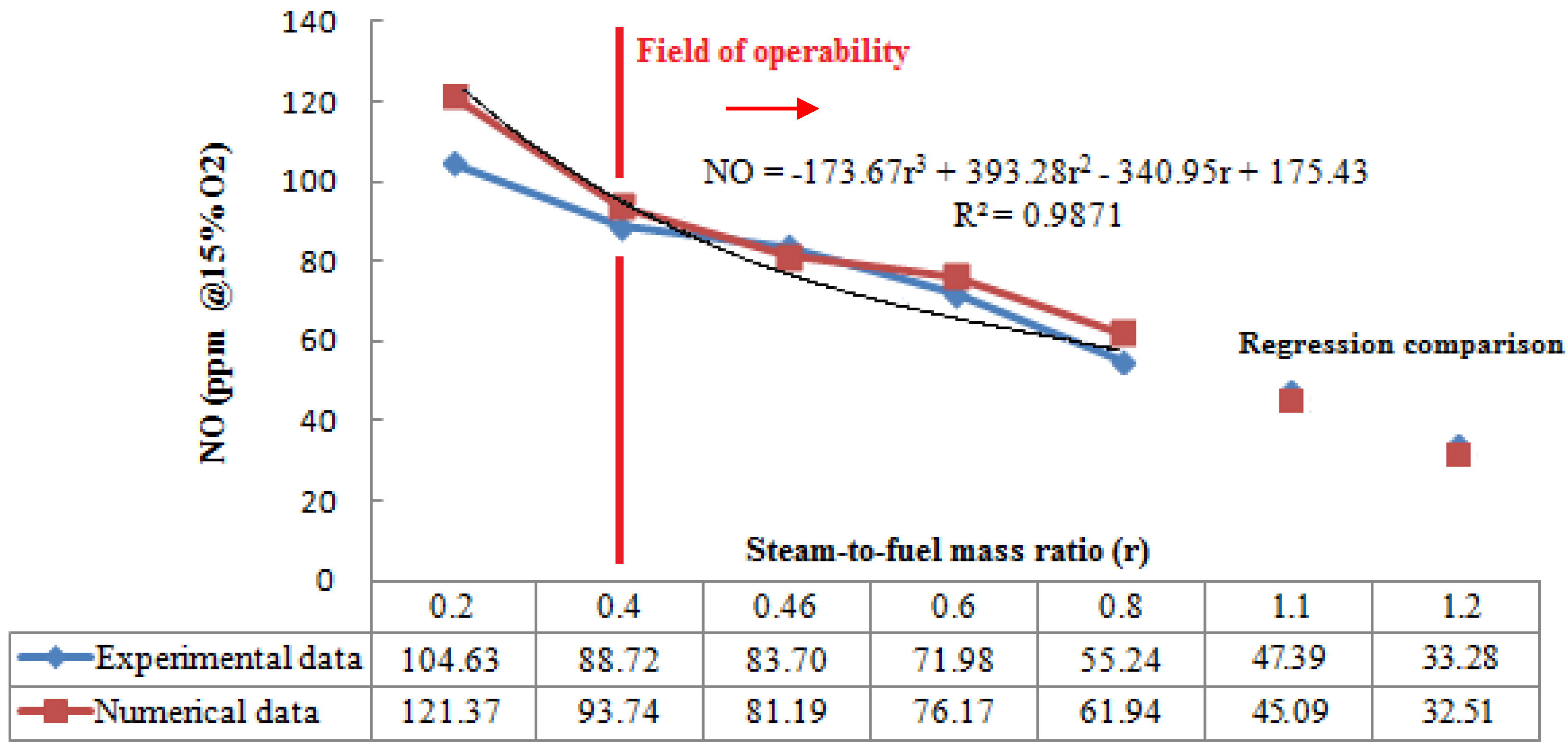
To completely evaluate the pollutant emissions, the effect of different mass flow rates of steam injected within the combustion chamber has been studied at full load and ISO condition, also. In a STIG (STeam Injected Gas Turbine) cycle, the amount of injected steam represents a sensible parameter to take into account, since there are practical limits to the amount of steam, as well as water that can be injected into the combustor before a serious flame stability problems occur [12]. This has been experimentally determined and must be taken into account in all applications if the combustor is to ensure low NOx emissions and long hardware life for the gas turbine user. In ordinary operating conditions, the steam-to-fuel mass ratio (r) is between 0.2 and 0.8. The results shown in Figure 6 for NOx have been plotted taking this range as the reference (r = 0.46 represents the design value).
Figure 6.
NOx emission vs. steam-to-fuel mass ratio.

It is evident how the computational model has a good agreement with experimental results, primarily for intermediate values of r (0.4 ˂ r ˂ 0.6). For values close to the minimum, the code tends to produce a higher percentage of errors at about 15%. These discrepancies could be related to experimental uncertainties in input parameters to the computations that can be amplified in the case of extremely low values of this parameter, producing an overestimation of temperature within the flame zone. If this error cannot be considered tolerable, the field of operability is limited to a steam-to-fuel-mass ratio higher than 0.4; in fact, lower error percentages have been obtained for the other operating conditions within the whole simulated range.
The model analysis has been extended for higher values of r, which are usually adopted just when an increase of electrical power is required. A third order regression curve, built through the numerical data, has been used in the cases of r = 1.1 and r = 1.2. The comparison with experimental data provides an excellent fitting, since very limited differences can be noticed. These results confirm that the software prediction capability can be extended to extremely high values for steam mass flow rate.
The effect of steam injection on CO emission is almost negligible. Steam temperature is very similar to the air temperature, so that experimental data at nominal conditions show no appreciable variations with increasing r. From a numerical point of view, the employed UDF cannot consider the influence of r, because there is no parameter that depends on the steam mass flow rate.
4.1.1. Thermal and Fluid Dynamic Internal Fields
Since the previous study demonstrated the validity of the present CFD model, it is interesting to analyze some physical characteristics of the internal fields of the combustion chamber. Figure 7a shows the temperature contour plot on the symmetry plane of the burner and on a cutting plane in the dilution zone. Different peculiarities of a non-premixed combustion can be highlighted. First of all, the flame occupies the central and terminal part of the burner, since the chemical species need time for mixing and complete reactions: the primary zone is characterized by the low temperature of the mixture, since the reaction rate is limited by a high mass fraction of the fuel (Figure 7b).
Figure 7.
(a) Temperature contour plot for a secondary zone cross-section (Left) and the symmetry plane (Right); (b) Methane concentration within the primary zone.
Figure 7.
(a) Temperature contour plot for a secondary zone cross-section (Left) and the symmetry plane (Right); (b) Methane concentration within the primary zone.

Secondly, the flame develops into a thin interface with the air flux and produces a compact body flame: this structure is typical of the diffusive reaction mechanism. The cutting plane on the dilution zone allows one to verify the influence of the cold air flux in preserving walls and decreasing the temperature of exhaust gases before the first stage of the gas turbine.
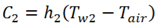
The strong connection between the temperature field and the NOx production rate is evident in Figure 8, where three different cross-sections have been plotted. Numerical simulations reveal that the distribution of maximum values follow the flame shape within the secondary zone of the combustion chamber where temperature range exceeds 2,000 K.
Keeping attention on fluid dynamics, one of the most important parameters that can be verified is the Mach number of the methane jet (Figure 9). These kind of combustion chambers are not designed to operate with supersonic gaseous jets, and simulations confirm that the injection is characterized by a supersonic flow just near the injectors’ discharge. The delaying action of the air involves a decreasing of the Mach number in the range between 0.5 and 0.8, already within the primary zone.
Figure 8.
NOx production rate on the symmetry plane and on two different normal x cuts.
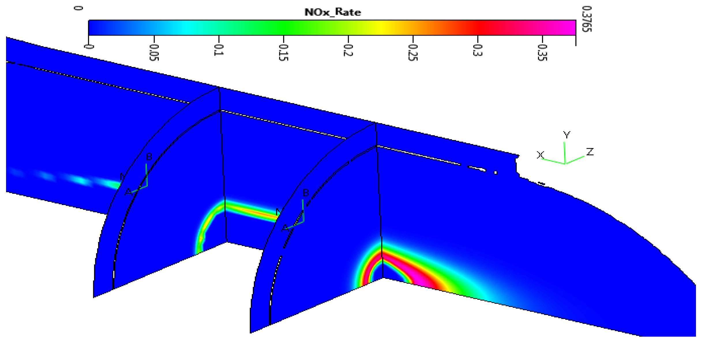
Figure 9.
Fuel Mach number: contour plot and chart.
Figure 10 reports the stream lines and the y-direction velocity contour plot in a cross-section at the beginning of the primary zone. It is evident how the CFD model can describe the recirculation flow at the inlet of the combustion chamber. This is an important phenomenon to take into account, because it influences the pressure losses and the mixing process between reactants.
Figure 10.
Recirculation zone.
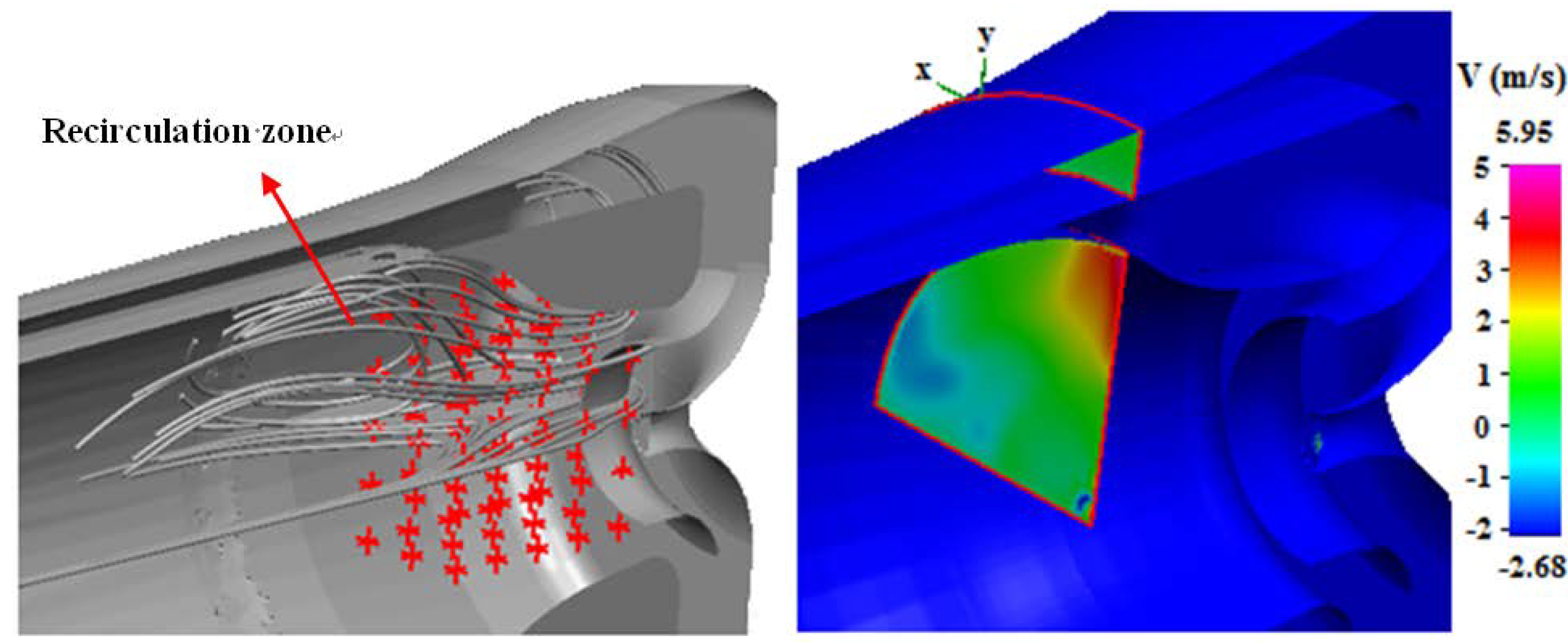
From this point of view, the attention has been focused on the Mach number and recirculation flow to characterize the primary zone, since the employed correlation for CO contains the assessment for Tpz, which is directly influenced by fuel distribution and fluid dynamics. Good results in CO estimation are primarily related to the ability of the model to describe these phenomena.
4.2. Experimental and Numerical Results at Partial Load
As mentioned earlier, the analysis has been extended to 75, 80 and 90% of the nominal thermal power. Figure 11 shows the comparison between the computed temperatures and the measured values at the discharge of the combustion chamber. The decreasing trend in temperature is the result of the combination of both the air and fuel lower mass flow rate, due to the (IGV) regulation at the compressor intake. The numerical simulations can provide, in any case, a good agreement with the experimental data, with a maximum value of the error lower than 4%.
Figure 11.
Discharge temperature at different loads.
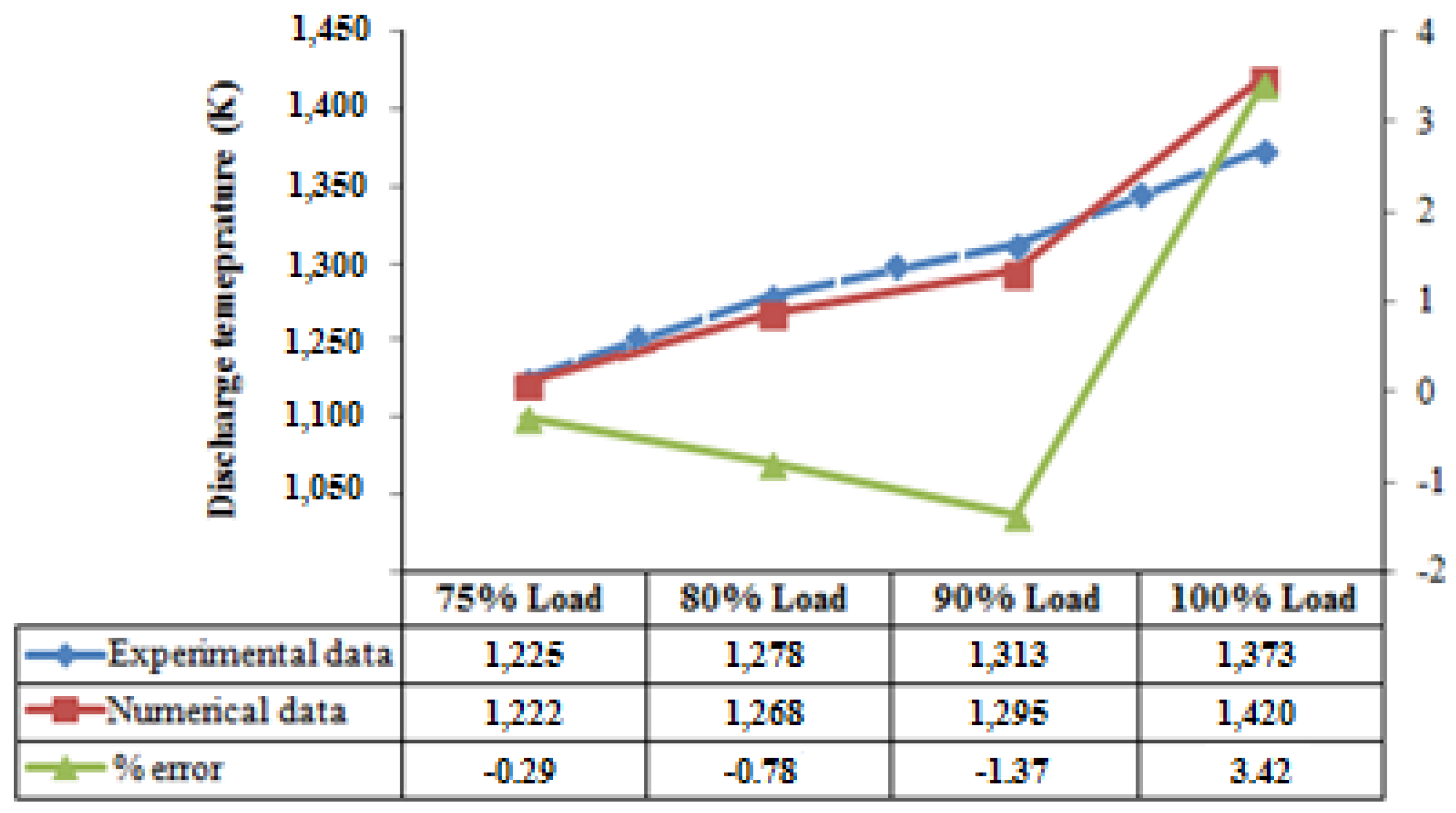
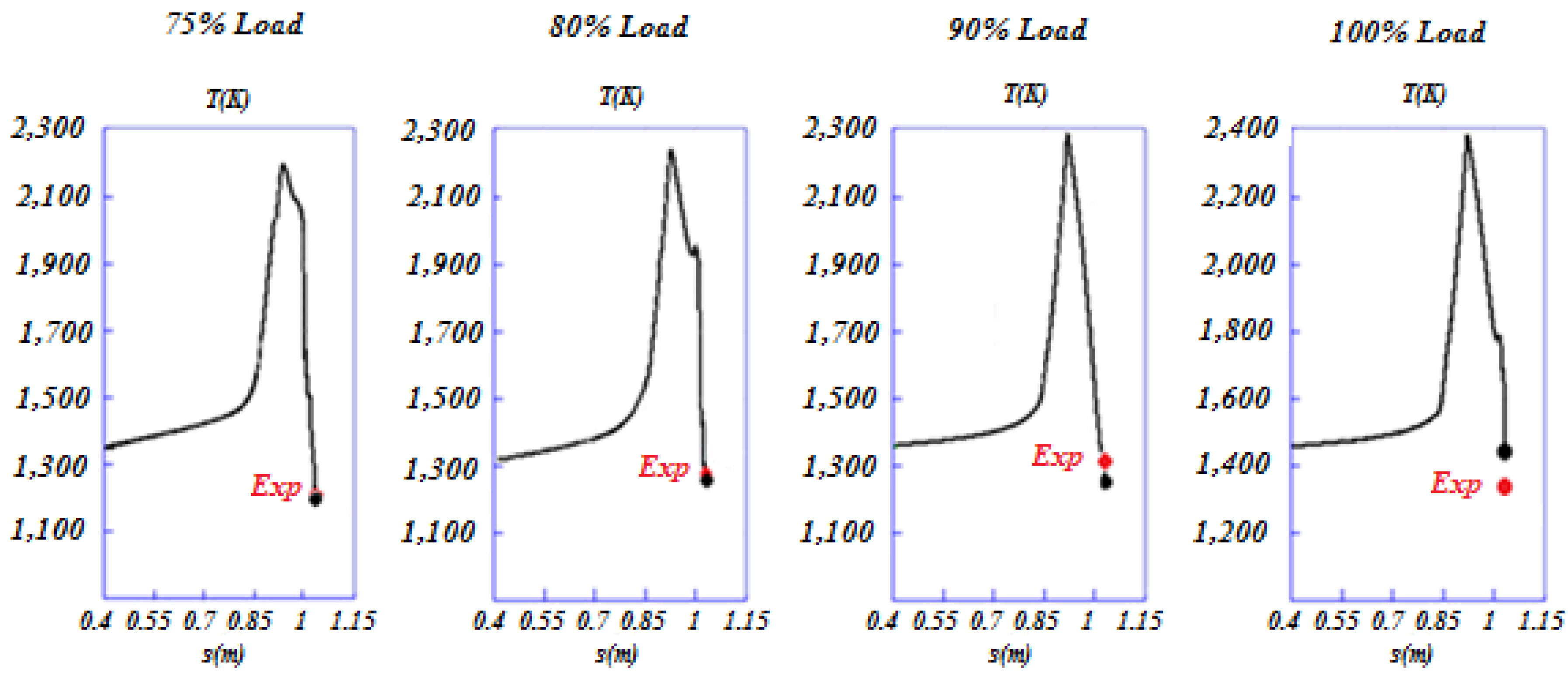
Figure 12 reports the averaged temperature for each cross-section within the intermediary and secondary zones of the combustion chamber: the rough rising in temperature due to the completion of the fuel oxidation is followed by a fast cooling due to the action of the fresh air entering from the dilution zone and the decreasing of the body flame diameter, as can be seen in Figure 7a. In general, the presence of IGV as a power control system has a slight effect on the NOx emissions; in fact, the IGV maintains a high exhaust temperature also at partial load conditions, so that the NOx concentration can vary by a few ppm.
Figure 12.
Comparison between numerical and experimental temperatures at different load values.

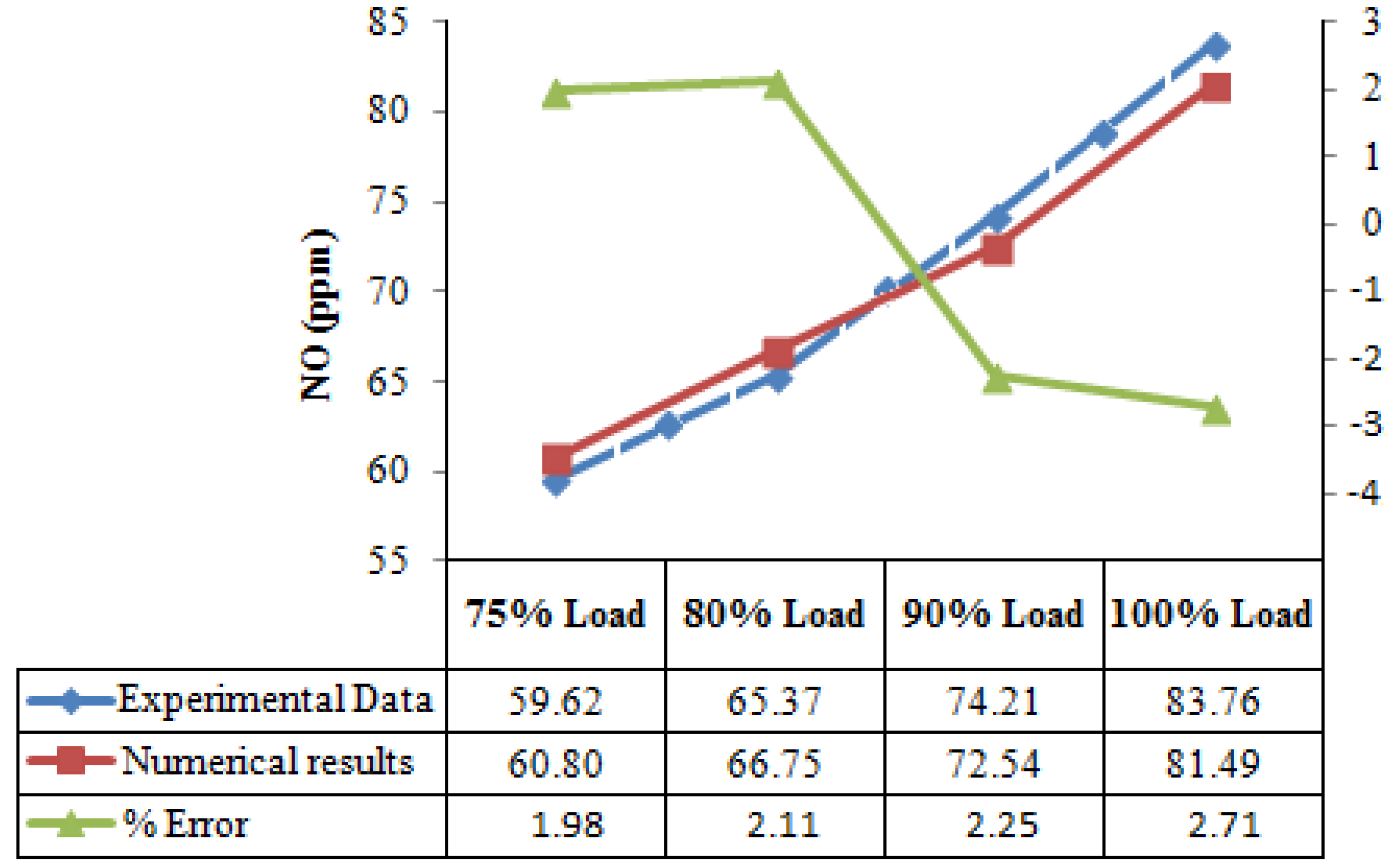
However, for the studied cases, the decreasing of the temperature peak reached within the combustion chamber determines a reduction in terms of NOx pollutant emissions. This trend is well described also by the numerical model (Figure 13): as NOx strongly depends on temperature, this is an indication that the model can provide an averaged internal thermal field close to the real one.
Figure 13.
NOx prediction at different load values.

The evaluation of the numerical model performance in terms of CO assessment at partial load has been summarized in Figure 14. First of all, it is important to underline that the model can predict the increasing in CO emissions, due to the reduction of the peak temperatures within the combustion chamber. However, as well as is seen in the analysis dedicated to the full load condition, also in this case, the software tendency is to overestimate the carbon monoxide concentration at the discharge section of the burner.
Figure 14.
CO prediction at different load values. UDF, user-defined function.
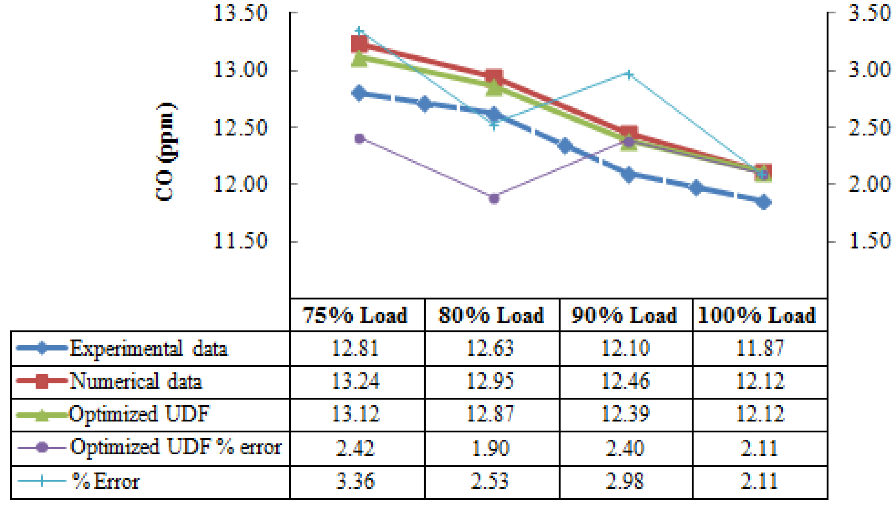
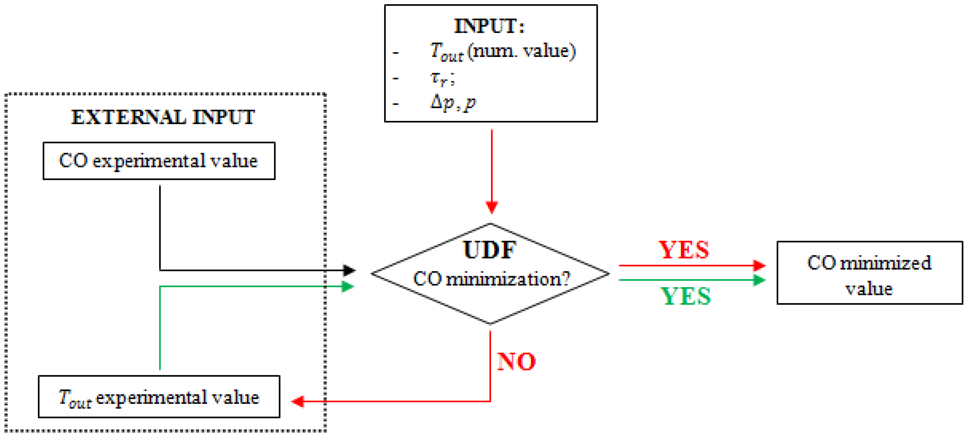
To improve the UDF and minimize the error, a hybrid strategy can be adopted (Figure 15): while the numerical temperature, , is directly transferred to the UDF, the experimental value of temperature and experimental CO concentration can be given as the external input. In this way, the code can compute Equation (6) choosing the temperature that minimizes the difference with the experimental value. This approach reduces the error when the estimated temperature is lower than the real one, and it has the advantage of directly joining together the code with real data.
Figure 15.
UDF flow chart for the CO minimization.

5. Conclusions
In this paper, a numerical model for the prediction of pollutant emissions within a Frame 6B combustion chamber was presented. The analysis involved both nominal and partial load conditions in order to completely evaluate the setting of the models that have been implemented. Furthermore, a sensitive analysis was developed varying the intake temperature of the air and the steam to the fuel mass ratio at full load.
The real discharge temperature was used for a direct comparison with the numerical result: in any case, the differences provided negligible percentage errors. As to the internal temperature field, there is no experimental data available; its numerical analysis confirmed some peculiarities of non-premixed diffusion combustion, such as the body flame structure and the mixing phenomena between reactants. However, an indirect control is possible analyzing the NOx emissions at the outlet section of the combustion chamber. In fact, excluding the results obtained for extremely low values of the steam-to-fuel mass ratio, NOx concentrations have a good agreement with experimental results. Therefore, it can be concluded that also the thermal-fluid-dynamic field within the burner reflects the real phenomenon. A regression numerical curve was also obtained to compute NOx for a high steam mass flow rate, producing an excellent fitting with real data.
Ritz and Mongia correlation was implemented through an innovative UDF for CO computing. Even if the discrepancies with the experimental data are always acceptable, a systematic overestimation was verified at both nominal and partial load. In this latter case, the influence of discharge temperature on calculation was studied: instead of the numerical temperature, the experimental value was used to improve the code and limit the percentage error.
Acknowledgments
The author wishes to acknowledge Cofely GDF SUEZ S.p.A for experimental data related to the power plant located in Nera Montoro (Narni, Italy) and Esi-Group for technical support.
Conflicts of Interest
The author declares no conflict of interest.
References
- Ol’Khovskii, G.G. Prospective gas turbine and combined-cycle units for power engineering (A review). Therm. Eng. 2013, 60, 79–88. [Google Scholar] [CrossRef]
- Lefbvre, A.H.; Ballal, D.R. Gas Turbine Combustion—Alternative Fuels and Emissions, 3rd ed.; CRC Press: Boca Raton, FL, USA, 2010; pp. 153–154. [Google Scholar]
- Stöhr, M.; Arndt, C.M.; Meier, W. Effects of Damköhler number on vortex-flame interaction in a gas turbine model combustor. Proc. Combust. Inst. 2013, 34, 3107–3115. [Google Scholar] [CrossRef]
- Strakey, P.A.; Eggnspieler, G. Development and validation of a thickened flame modeling approach for large eddy simulation of premixed combustion. J. Eng. Gas Turbine Power 2010, 132, 1–9. [Google Scholar]
- Smith, G.P.; Golden, D.M.; Frenklach, M.; Moriarty, N.W.; Eiteneer, B.; Goldenberg, M.; Bowman, T.C.; Hanson, R.K.; Song, S.; Gardiner, W.C.; et al. Gri-Mech 3.0. Available online: http://www.me.berkeley.edu/gri_mech/ (accessed on 10 October 2012).
- Ianni, J. A comparison of the Bader-Deuflhard and the Cash-Karp Runge-Kutta. Integrators for the GRI-MECH 3.0 Model Based on the Chemical Kinetics Code Kintecus. In Computational Fluid and Solid Mechanics 2003; Bathe, K.J., Ed.; Elsevier Science Ltd.: Oxford, UK, 2003; pp. 1368–1372. [Google Scholar]
- Kong, S.; Han, Z.; Reitz, R.D. The Development and Application of a Diesel Ignition and CombustionModel for Multidimensional Engine Simulation; SAE Technical Paper 950278; SAE International: Detroit, MI, USA, 1995. [Google Scholar]
- Baritaud, T. Multi-Dimensional Simulation of Engine Internal Flow, 1st ed.; Technip: Rueil-Malmaison, France, 1998; pp. 234–237. [Google Scholar]
- Aïssani, S.; Bouam, A.; Kadi, R. Combustion chamber steam injection for gas turbine performance improvement during high ambient temperature operations. J. Eng. Gas Turbine Power 2008, 130, article number 041701. [Google Scholar]
- Gülder, O.L. Flame temperature estimation of conventional and future jet fuels. J. Eng. Gas Turbine Power 1986, 108, 376–380. [Google Scholar] [CrossRef]
- ACE+ Suite 2011, Theory Guide. 2011.
- Srinivas, T.; Gupta, A.V.S.S.K.; Reddy, B.V. Parametric simulation of steam injected gas turbine combined cycle. Proc. Inst. Mech. Eng. Part A J. Power Energy 2007, 221, 873–883. [Google Scholar] [CrossRef]
© 2013 by the authors; licensee MDPI, Basel, Switzerland. This article is an open access article distributed under the terms and conditions of the Creative Commons Attribution license (http://creativecommons.org/licenses/by/3.0/).
Share and Cite
MDPI and ACS Style
Meloni, R. Pollutant Emission Validation of a Heavy-Duty Gas Turbine Burner by CFD Modeling. Machines 2013, 1, 81-97. https://doi.org/10.3390/machines1030081
AMA Style
Meloni R. Pollutant Emission Validation of a Heavy-Duty Gas Turbine Burner by CFD Modeling. Machines. 2013; 1(3):81-97. https://doi.org/10.3390/machines1030081
Chicago/Turabian StyleMeloni, Roberto. 2013. "Pollutant Emission Validation of a Heavy-Duty Gas Turbine Burner by CFD Modeling" Machines 1, no. 3: 81-97. https://doi.org/10.3390/machines1030081