Optimal B-Spline Bases for the Numerical Solution of Fractional Differential Problems


Dept. SBAI, Università di Roma “La Sapienza”, Via Antonio Scarpa 16, 00161 Roma, Italy
Axioms 2018, 7(3), 46; https://doi.org/10.3390/axioms7030046
Submission received: 14 May 2018
/
Revised: 17 June 2018
/
Accepted: 22 June 2018
/
Published: 2 July 2018
(This article belongs to the Special Issue Advanced Numerical Methods in Applied Sciences)
Abstract
:Efficient numerical methods to solve fractional differential problems are particularly required in order to approximate accurately the nonlocal behavior of the fractional derivative. The aim of the paper is to show how optimal B-spline bases allow us to construct accurate numerical methods that have a low computational cost. First of all, we describe in detail how to construct optimal B-spline bases on bounded intervals and recall their main properties. Then, we give the analytical expression of their derivatives of fractional order and use these bases in the numerical solution of fractional differential problems. Some numerical tests showing the good performances of the bases in solving a time-fractional diffusion problem by a collocation–Galerkin method are also displayed.
1. Introduction
In the last few decades, fractional calculus has proved to be a powerful tool for describing real-world phenomena. Differential problems of fractional order, initially introduced to model anomalous diffusion in viscoelastic materials, are now used in several fields, from physics to population dynamics, from signal processing to control theory [1,2,3,4,5]. For an introduction of fractional calculus, we refer to [6,7,8,9].
As fractional differential models have become widespread, the development of efficient numerical methods to approximate their solution has become of primary interest. In fact, the nonlocality of the fractional derivative poses a severe challenge in its approximation, and, to face this problem, several numerical methods were proposed in the literature. For a review on numerical methods, see, for instance, [10,11,12,13,14,15].
In particular, we are interested in the solution of differential problems on bounded intervals. In this case, it is important to have a function basis available that naturally fulfills boundary and/or initial conditions and does not show numerical instabilities at the boundaries. From this point of view, B-spline bases are especially suitable and their use in the numerical solution of classical differential problems is widely diffused (see, for instance, [16,17,18]). Despite the indubitable success of these methods, the use of B-spline bases for the solution of differential problems of fractional order is not yet very common and limited to few examples. For instance, in [19], the authors used a linear B-spline basis to solve a multi-order fractional differential problem by the operational matrix method, while, in [20], a collocation method based on cubic B-spline wavelets was constructed to solve ordinary differential equations of fractional order.
The aim of this paper is to show how optimal B-spline bases can be profitably used for the solution of fractional differential problems. To this end, we not only describe in detail the construction of optimal B-spline bases of any degree but also give the analytical expression of the basis functions and of their fractional derivatives. These expressions are an efficient tool to construct numerical methods based on spline functions.
The paper is organized as follows. In Section 2, we show how to construct polynomial B-spline bases and recall their main properties. In particular, the construction of cardinal B-splines on the real line through the divided difference operator is described in Section 2.1 and Section 2.2, while, in Section 2.3, we show how to construct optimal B-spline bases on bounded intervals. Their analytical expression in case of equidistant nodes is given in Section 2.4. Section 2.5 is devoted to the evaluation of the fractional derivatives of the B-spline bases. Finally, in Section 2.6, we show how to use optimal bases for the numerical solution of a time-fractional diffusion problem by a collocation–Galerkin method. In Section 3, we use the optimal B-spline basis of degree 3 to solve some test problems; some numerical results are also displayed. Section 4 contains a discussion on the results and highlights possible extensions.
2. Materials and Methods
In this section, we define the B-spline bases through the divided difference operator and recall their main properties. Then, we give the analytical expression of the basis functions and of their fractional derivatives. Finally, B-spline bases are used to solve a fractional differential problem by a collocation–Galerkin method.
2.1. The Divided Difference Operator
Let
be a sequence of simple, i.e., non coincident, knots and let
be the determinant of the collocation matrix
associated with the function system and the knot sequence (1).
The divided difference operator of a function f over the knots is defined as
The formula above can be generalized to the case of coincident knots as follows. Let the knots occur more than once, i.e.,
and let
be the multiplicities of the coincident knots, i.e.,
where are the non coincident knots of the sequence .
Assuming the functions in are sufficiently smooth, the collocation matrix associated with the function system over the knot sequence (7) is given by
2.2. The Cardinal B-Splines
The polynomial splines are piecewise polynomials having a certain degree of smoothness which is related to the degree of the polynomial pieces. Spline functions can be represented as a linear combination of B-splines that form a local basis for the spline spaces [21].
The cardinal B-splines, i.e., the polynomial B-splines having break points on integer knots, can be defined by applying the divided difference operator (4) to the truncated power function defined as
Then, the cardinal B-spline of degree n on the integer knots
is given by
where is the finite difference operator
From the above definition, it follows that the cardinal B-spline is compactly supported on , positive in and belongs to . Moreover, the system of the integer translates
forms a function basis that is a partition of unity, i.e.,
and reproduces polynomials up to degree n [21].
The basis can be generalized to any set of equidistant knots , where is the space step, by scaling, i.e.,
For details and further properties on polynomial B-splines, see, for instance, [21].
It is always possible to construct bases on bounded intervals by restricting the B-spline basis on an interval . However, in this way, we obtain bases that could be numerically unstable since the functions at the boundaries are obtained by truncation. Moreover, boundary or initial conditions are not easy to satisfy. In the following section, we will show how to construct stable bases on the interval that easily satisfy boundary or initial conditions.
2.3. Optimal B-Spline Bases
Optimal B-spline bases on bounded intervals can be defined by introducing multiple knots at the boundaries of the given interval [21].
Let be an integer and let be the sequence of the integer knots of the interval . We extend to a sequence of knots by introducing knots of multiplicity at the boundaries of the interval, i.e.,
The functions of the optimal B-spline basis
of degree n with knots are given by the divided difference
so that each function has compact support with
From (19), it follows that the basis has interior functions, i.e., the functions , having all simple knots, and edge functions, i.e., the functions for and that have a multiple knot at the left or right boundary, respectively.
The basis is centrally symmetric, i.e.,
Moreover, the functions satisfy the boundary conditions
where denotes the usual derivative of integer order r.
Finally, the basis forms a partition of unity, i.e.,
and is stable, i.e., for any sequence with it holds
where
is the condition number of the basis . From (25), it follows that where denotes a perturbation of the sequence c. As a consequence, optimal B-spline bases are numerically stable so that numerical errors are not amplified when evaluating spline approximations.
The basis can be generalized to any sequence of equidistant knots on a bounded interval by mapping , i.e.,
where . The interior functions are the functions
while the edge functions are
2.4. Analytical Expression of the Optimal B-Spline Bases
Let be the optimal basis (18) associated with the knot sequence (17). The interior functions , , are the translates of the B-spline having support , i.e.,
The left edge functions , , having support on , can be evaluated by using the finite difference operator (9) for coincident knots. For , we get
By Definition (8), we get
where is the order diagonal matrix
is the dimension matrix
and is the order collocation matrix
Thus, for the numerator in the last equality of (31), we have
For the denominator, a similar calculation gives
where is the order collocation matrix
Theorem 1.
Proof.
The right edge functions , , having support , can be easily obtained recalling the symmetry property (21).
In the following corollary, we give the analytical expression of the first three left boundary functions.
Corollary 1.
Let be the sequence of multiple knots (17) on the interval . For , the left edge functions are given by
It is interesting to observe that , . In particular, when (linear case), there is just one left edge function and the basis coincides with the basis restricted to the interval I. We recall that the basis is the unique interpolatory B-spline basis.
2.5. Fractional Derivatives of the Optimal B-Spline Bases
In this section, we give the explicit expression of the derivatives of fractional order of the functions in the basis .
Let be the Euler’s gamma function
Definition 1.
Assuming f is a sufficiently smooth function, the Caputo fractional derivative of f is defined as
Definition 2.
The Riemann–Liouville fractional derivative of a function f is defined as
We recall that the Caputo derivative and the Riemann–Liouville derivative can be obtained from each other by
If f satisfies homogeneous initial conditions, i.e., , , the Riemann–Liouville derivative coincides with the Caputo derivative.
To use the basis for the solution of differential problems of fractional order, we need the expression of the fractional derivatives of the functions .
The derivatives of the interior functions can be easily evaluated by the differentiation rule
where is the finite difference operator (13) [15,24]. Since satisfies homogeneous boundary conditions, the Riemann–Liouville derivative is equal to the Caputo derivative.
Theorem 2.
The Caputo derivative of the left edge functions are given by
where
Proof.
First of all, we write the explicit expression of the matrix , i.e.,
From (39), we get The claim follows by expanding the determinant of along the last column. ☐
Thus, to evaluate the fractional derivatives of the edge functions, we need the fractional derivatives of the translates of the truncated power function. By Definition (44), we get
Integration rules for rational functions give [25]
where is the Heaviside function and is the hypergeometric function
with denoting the rising Pochhammer symbol
Since , is actually a finite sum, i.e.,
Moreover, can be evaluated by a direct calculation, i.e.,
Thus, we get the analytical expression of the Caputo derivative (cf. also [20]).
Theorem 3.
For with and m a positive integer, the Caputo derivative of the translates of the truncated power function is given by
The Riemann–Liouville derivatives of the functions can be obtained by the Caputo derivatives using the initial conditions (22) in Equation (46).
2.6. The Collocation-Galerkin Method
In this section, we show how to use the optimal basis introduced in the previous sections to solve a fractional differential problem, i.e., the time-fractional diffusion problem (cf. [26,27,28])
where , , denotes the partial Caputo derivative with respect to the time t.
Let
where is the approximating space generated by the optimal B-spline basis
of the interval on equidistant knots with space step (cf. (27)). We observe that the basis naturally satisfies the homogeneous boundary conditions
For any h held fix, the spline Galerkin method looks for an approximating function
that solves the variational problem
where . Writing (62) in a weak form and using (61), we get the system of fractional ordinary differential equations
with initial condition
Here, is the unknown function vector, is the mass matrix, is the stiffness matrix and is the load vector whose entries are
The entries of Q and L can be evaluated explicitly by using the integration and differentiation rules for B-splines [21]. The entries of F can be evaluated by quadrature formulas especially designed for Galerkin methods [29].
Now, we introduce the sequence of temporal knots. Let
where with the time step, be a set of equidistant nodes in the interval having a knots of multiplicity at the left boundary. We assume the unknown functions belong to the spline space
so that
We observe that just the functions , , are boundary functions while all the other functions in the basis are cardinal B-splines.
To solve the fractional differential system (63), we use the collocation method on equidistant nodes introduced in [28,30]. Let with be a set of non coincident collocation points in the interval . Then, collocating (63) on the nodes , we get the linear system
where is the unknown vector,
are collocation matrices, and . When , (68) is a square linear system and the collocation matrix A is non singular if and only if [21],
while B is always non singular [31]. Otherwise, (68) is an overdetermined linear system that can be solved in the least squares sense.
We notice that we must pay a special attention to the evaluation of the entries of A since they involve the values of the fractional derivative in the collocation points. This can be done by the differentiation rules given in Section 2.5.
3. Results
To test the performance of the optimal B-spline basis when used to solve fractional differential problems, we solved the time-fractional diffusion problem (57) by the collocation–Galerkin method described in Section 2.6. In the tests, we used the optimal basis having degree 3 since the cubic B-spline has a small support but is sufficiently smooth. In fact, the cubic B-spline belongs to and its support has length 4. In particular, the basis has 3 right (left) edge functions with support (), , while the interior functions have support , . In the following section, we give the analytical expression of the functions and of their fractional derivatives; then, we show some numerical results.
3.1. The Optimal B-Spline Basis of Degree
When , we get the cubic B-spline basis. The optimal B-spline basis of the interval , with L an integer greater than 3, is associated with the sequence of integer knots
with , , , . has interior functions and six edge functions, three for each boundary.
The interior functions , , are the translates of the cubic cardinal B-spline, i.e.,
where
From Corollary 1, it follows that the three left edge functions , , are given by
Now, using Theorems 3, we obtain the analytical expression of the Caputo derivative of fractional order of the translates of the truncated power function
Thus, substituting (78) in (48), we get
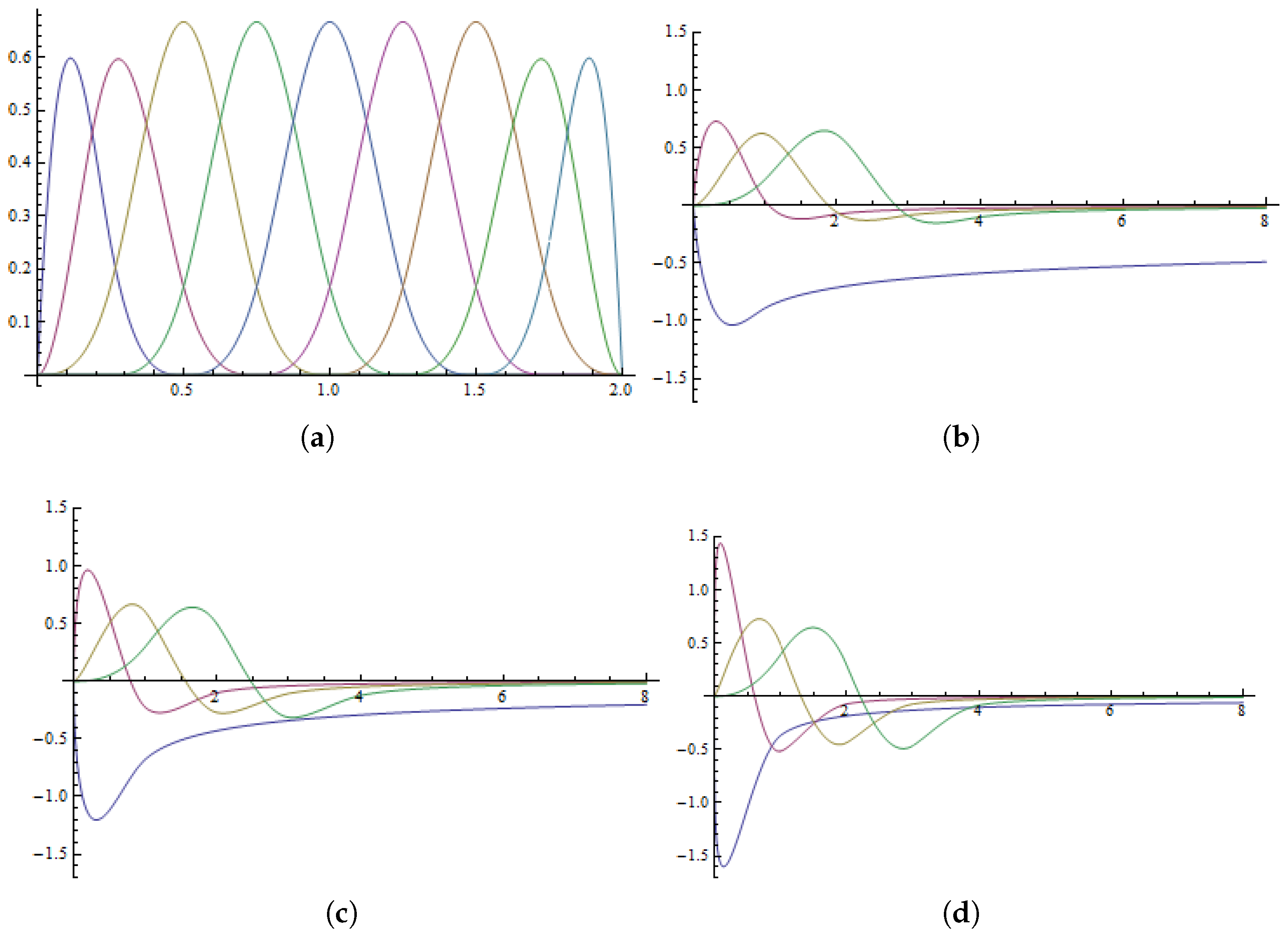
The optimal basis and its fractional derivatives in case of equidistant knots on an interval can be evaluated by scaling as shown in (27)–(29). The optimal B-spline basis in the interval for is shown in Figure 1a. The Caputo derivatives of fractional order are shown in Figure 1b–d.
To give an idea of the condition number of the discretization matrix (cf. (68)), in Table 1, Table 2 and Table 3, we list the condition number of the matrix when using the cubic B-spline basis for different values of the order of the fractional derivative and different values of the space and time steps.
3.2. Numerical Tests
In this section, we show the numerical results we obtained when solving the differential problem (57) for three different expressions of the known term and different values of the fractional derivative. In the tests, we set and and chose as collocation nodes the equidistant points of the interval with time step . All the tests were performed in the Mathematica environment [32].
3.2.1. Test 1
To test the accuracy of the method, we first solved the time-fractional diffusion Equation (57) when
In this case, the exact solution is the bivariate polynomial
Since the cubic B-spline basis reproduces polynomials up to degree 3, the approximation error of the collocation–Galerkin method is zero so that we expect the numerical solution coincides with the exact solution.
We evaluated the numerical solution for , and and different values of the order of the time fractional derivative .
Let us define the error by
where denotes the numerical solution of the fractional differential system (63) obtained by the collocation method.
The tests show that, as expected, the error is on the order of the machine precision even using a large step size. The numerical solution and the error for are shown in Figure 2.
3.2.2. Test 2
To test the accuracy of the method when approximating time fractional derivatives, we solved the time-fractional diffusion Equation (57) for
where is the Kummer’s confluent hypergeometric function
where (cf. [9]). In this case, the exact solution is
so that the error for the spatial approximation is negligible.
The -norm of the error
and the numerical convergence order
are listed in Table 4. The numerical solution in the case when obtained for , and is shown in Figure 3.
The numerical results show that the method converges with convergence order approximatively equal to 4 and gives a good approximation even using few collocation points. Moreover, the accuracy of the numerical solution does not depend on the order of the fractional derivative.
3.2.3. Test 3
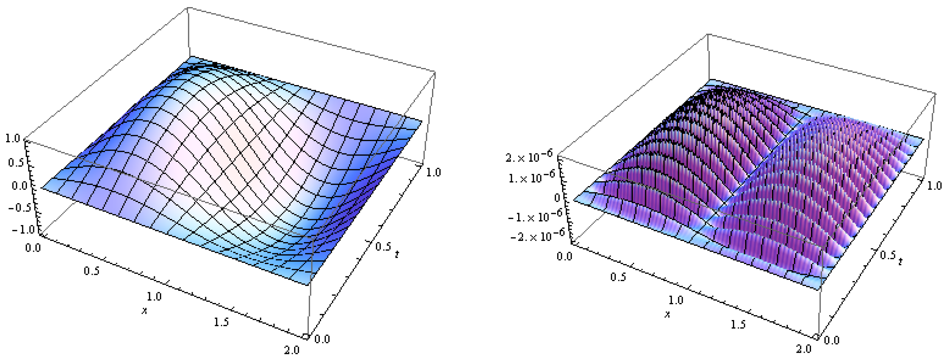
Finally, we solved the time-fractional diffusion equation (57) for
In this case, the exact solution is
The -norm of the error and the numerical convergence order
are listed in Table 5. The numerical solution in the case when obtained for and is shown in Figure 4.
Also in this case, the numerical solution has a good accuracy that is not affected by the order of the fractional derivative. The numerical convergence order is approximatively 4.
4. Discussion
In this paper, we showed how optimal B-spline bases have good approximation properties that make them particularly suitable to be used in the solution of fractional differential problems. First of all, boundary and initial conditions can be satisfied easily in view of properties (22)–(23) so that the numerical solution we obtained does not suffer from the numerical instabilities near the boundaries that appear when truncated functions at the boundaries are used (cf. [28]). Moreover, optimal B-spline bases are stable (cf. (25)) meaning that numerical errors are not amplified. Nevertheless, Table 1, Table 2 and Table 3 show that the condition number of the discretization matrix increases as the dimension of the matrix increases. The conditioning gets worse when the order of the fractional derivative becomes smaller. In this case, the linear system (68) can be accurately solved by Krylov methods [33].
As for the convergence order, we observe that several methods proposed in the literature to solve fractional differential problems have convergence order that depends on the order of the fractional derivative (see, for instance, [26,27]). In the case of the cubic B-spline basis, the numerical tests show that the numerical convergence order does not depend on the order of the fractional derivative being close to 4 for any value of . This result is in line with the Strang–Fix theory for classical differential problems [34]. We expect that the convergence order for the optimal B-spline basis is so that it can be increased easily by increasing the degree of the basis. In fact, optimal bases of high degree and their fractional derivatives can be evaluated by using the analytical expression given in Section 2.4 and Section 2.5. As far as we know, the analytical expressions (39) and (48) are new and, together with (27)–(29), are an easy tool to evaluate optimal B-spline bases on any set of equidistant knots on bounded intervals. Finally, we observe that the accuracy of the numerical solution we obtained is higher than the accuracy obtained in [26] where a quadrature formula was used to approximate the time fractional derivative and a finite element method was used for the spatial approximation.
The optimal bases we described can be used to solve other fractional differential problems, for instance problems involving the Riesz derivative [2], or can be used in other numerical methods, for instance in the operational matrix method or in wavelet methods. We notice that adaptive wavelet methods can be used to solve differential problems whose solutions are non smooth functions. Optimal bases generating multiresolution analyses and wavelet spaces can be obtained starting from a special family of refinable functions [35,36] so that the procedure described above can be generalized to other refinable bases.
Funding
This work was partially supported by grants University of Roma ”La Sapienza”, Ricerca Scientifica 2016 and INdAM-GNCS, Project 2018.
Conflicts of Interest
The author declares no conflict of interest.
References
- Hilfer, R. Applications of Fractional Calculus in Physics; World Scientific: Singapore, 2000. [Google Scholar]
- Kilbas, A.A.; Srivastava, H.M.; Trujillo, J.J. Theory and Applications of Fractional Differential Equations; Elsevier Science: North-Holland, The Netherlands, 2006. [Google Scholar]
- Sabatier, J.; Agrawal, O.; Tenreiro Machado, J.A. Advances in Fractional Calculus; Springer: Berlin, Germany, 2007. [Google Scholar] [CrossRef]
- Mainardi, F. Fractional Calculus and Waves in Linear Viscoelasticity: An Introduction to Mathematical Models; World Scientific: Singapore, 2010. [Google Scholar]
- Tarasov, V.E. Fractional Dynamics; Nonlinear Physical Science; Springer: Berlin, Germany, 2010. [Google Scholar] [CrossRef]
- Oldham, K.; Spanier, J. The Fractional Calculus; Academic Press: Cambridge, MA, USA, 1974. [Google Scholar]
- Samko, S.G.; Kilbas, A.A.; Marichev, O.I. Fractional Integrals and Derivatives; Gordon & Breach Science Publishers: Philadelphia, PA, USA, 1993. [Google Scholar]
- Podlubny, I. Fractional Differential Equations; Academic Press: Cambridge, MA, USA, 1998. [Google Scholar]
- Diethelm, K. The Analysis of Fractional Differential Equations: An Application-Oriented Exposition Using Differential Operators of Caputo Type; Springer: Berlin, Germany, 2010. [Google Scholar]
- Baleanu, D.; Diethelm, K.; Scalas, E.; Trujillo, J.J. Fractional Calculus: Models and Numerical Methods; World Scientific: Singapore, 2016. [Google Scholar]
- Li, C.; Chen, A.; Ye, J. Numerical approaches to fractional calculus and fractional ordinary differential equation. J. Comput. Phys. 2011, 230, 3352–3368. [Google Scholar] [CrossRef]
- Podlubny, I.; Skovranek, T.; Datsko, B. Recent advances in numerical methods for partial fractional differential equations. In Proceedings of the 2014 15th International Carpathian Control Conference (ICCC), Velke Karlovice, Czech Republic, 28–30 May 2014; pp. 454–457. [Google Scholar]
- Li, C.; Zeng, F. Numerical Methods for Fractional Calculus; CRC Press: Boca Raton, FL, USA, 2015; Volume 24. [Google Scholar]
- Li, C.; Chen, A. Numerical Methods for Fractional Partial Differential Equations. Int. J. Comput. Math. 2018, 95, 1048–1099. [Google Scholar] [CrossRef]
- Pitolli, F. A fractional B-spline collocation method for the numerical solution of fractional predator-prey models. Fractal Fractional 2018, 2, 13. [Google Scholar] [CrossRef]
- lHöllig, K. Finite Element Methods with B-Splines; SIAM: Philadelphia, PA, USA, 2003; Volume 26. [Google Scholar]
- Buffa, A.; Sangalli, G.; Vázquez, R. Isogeometric analysis in electromagnetics: B-splines approximation. Comput. Methods Appl. Mech. Eng. 2010, 199, 1143–1152. [Google Scholar] [CrossRef] [Green Version]
- Garoni, C.; Manni, C.; Serra-Capizzano, S.; Sesana, D.; Speleers, H. Spectral analysis and spectral symbol of matrices in isogeometric Galerkin methods. Math. Comput. 2017, 86, 1343–1373. [Google Scholar] [CrossRef]
- Lakestani, M.; Dehghan, M.; Irandoust-Pakchin, S. The construction of operational matrix of fractional derivatives using B-spline functions. Communi. Nonlinear Sci. Numer. Simul. 2012, 17, 1149–1162. [Google Scholar] [CrossRef]
- Li, X. Numerical solution of fractional differential equations using cubic B-spline wavelet collocation method. Communi. Nonlinear Sci. Numer. Simul. 2012, 17, 3934–3946. [Google Scholar] [CrossRef]
- Schumaker, L.L. Spline Functions: Basic Theory; Cambridge University Press: Cambridge, UK, 2007. [Google Scholar]
- Carnicer, J.M.; Peña, J.M. Totally positive bases for shape preserving curve design and optimality of B-splines. Computer Aided Geometric Design 1994, 11, 633–654. [Google Scholar] [CrossRef]
- Carnicer, J.M.; Peña, J.M. Total positivity and optimal bases. In Total Positivity and its Applications; Springer: Berlin, Germany, 1996; pp. 133–155. [Google Scholar]
- Unser, M.; Blu, T. Fractional splines and wavelets. SIAM Rev. 2000, 42, 43–67. [Google Scholar] [CrossRef]
- Gradshteyn, I.S.; Ryzhik, I.M. Tables of Integrals, Series and Products: Corrected and Enlarged Edition; Academic Press: New York, NY, USA, 1980. [Google Scholar]
- Ford, N.J.; Xiao, J.; Yan, Y. A finite element method for time fractional partial differential equations. Fractional Calculus Appl. Anal. 2011, 14, 454–474. [Google Scholar] [CrossRef] [Green Version]
- Li, X.; Xu, C. A space-time spectral method for the time fractional diffusion equation. SIAM J. Numer. Anal. 2009, 47, 2108–2131. [Google Scholar] [CrossRef]
- Pezza, L.; Pitolli, F. A fractional spline collocation-Galerkin method for the time-fractional diffusion equation. Commun. Appl. Ind. Math. 2018, 9, 104–120. [Google Scholar] [CrossRef] [Green Version]
- Calabrò, F.; Manni, C.; Pitolli, F. Computation of quadrature rules for integration with respect to refinable functions on assigned nodes. Appl. Numer. Math. 2015, 90, 168–189. [Google Scholar] [CrossRef]
- Pezza, L.; Pitolli, F. A multiscale collocation method for fractional differential problems. Math. Comput. Simul. 2018, 147, 210–219. [Google Scholar] [CrossRef]
- Forster, B.; Massopust, P. Interpolation with fundamental splines of fractional order. In Proceedings of the 9th International Conference on Sampling Theory and Applications (SampTa), Singapore, 2–6 May 2011. [Google Scholar]
- Wolfram Research, Inc. Mathematica, Version 8.0.4.0; Wolfram Research, Inc.: Champaign, IL, USA, 2011. [Google Scholar]
- Calvetti, D.; Pitolli, F.; Somersalo, E.; Vantaggi, B. Bayes meets Krylov: Statistically inspired preconditioners for CGLS. SIAM Rev. 2018, 60, 429–461. [Google Scholar] [CrossRef]
- Strang, G.; Fix, G. A Fourier analysis of the finite element variational method. In Constructive Aspects of Functional Analysis; Edizioni Cremonese: Naples, Italy, 1971; pp. 796–830. [Google Scholar]
- Gori, L.; Pitolli, F. Refinable functions and positive operators. Appl. Numer. Math. 2004, 49, 381–393. [Google Scholar] [CrossRef]
- Gori, L.; Pezza, L.; Pitolli, F. Recent results on wavelet bases on the interval generated by GP refinable functions. Appl. Numer. Math. 2004, 51, 549–563. [Google Scholar] [CrossRef]
Figure 1.
(a) the optimal B-spline basis in the interval for ; (b–d) the fractional derivatives (blue), (purple), (dark yellow), (green) of order (b), (c), (d).
Figure 1.
(a) the optimal B-spline basis in the interval for ; (b–d) the fractional derivatives (blue), (purple), (dark yellow), (green) of order (b), (c), (d).

Figure 2.
Test 1: (a) the numerical solution and (b) the error for and .
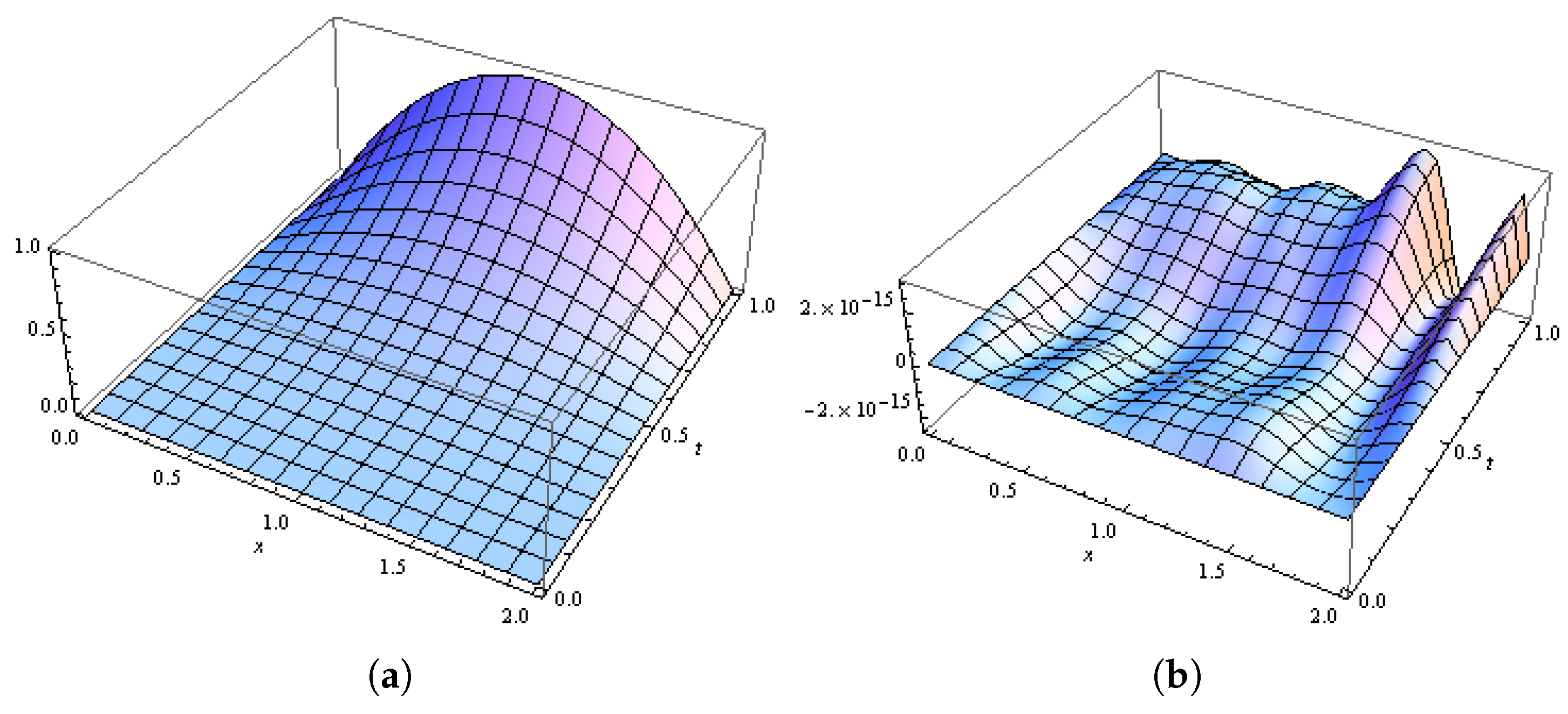
Figure 3.
Test 2: (a) the numerical solution and (b) the error in the case when and , , .
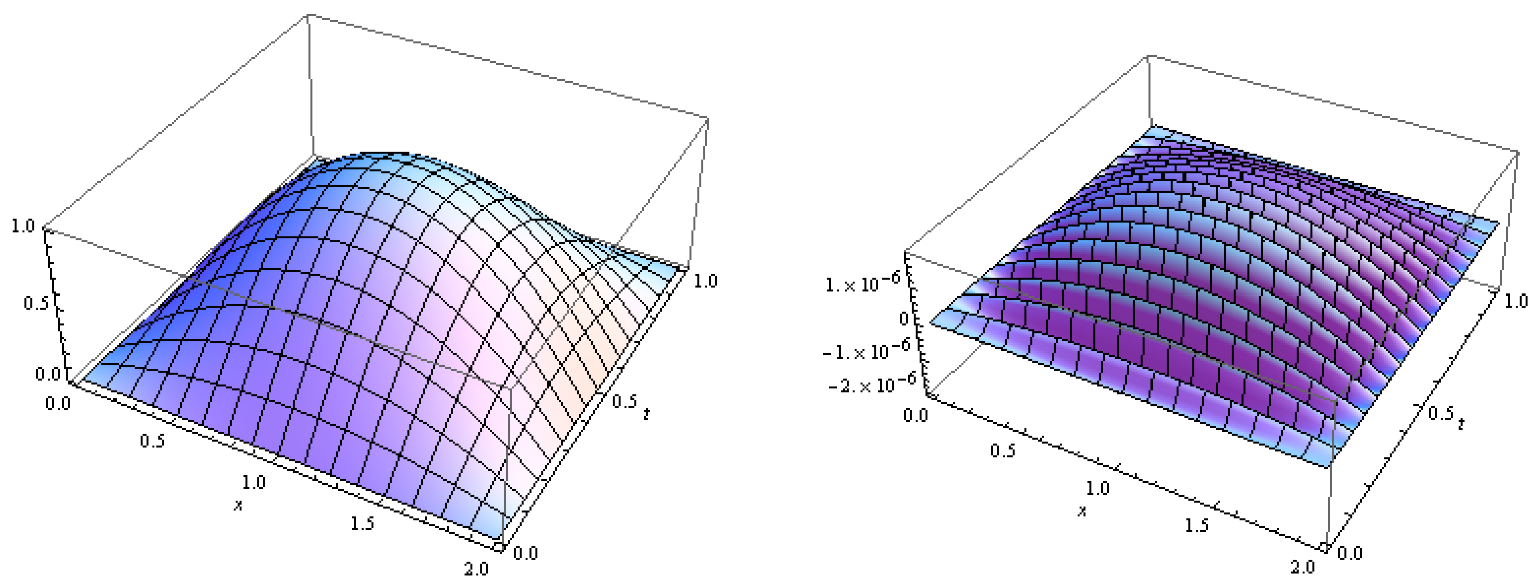
Figure 4.
Test 3: (a) the numerical solution and (b) the error for and , .

Table 1.
The condition number (rounded to the nearest integer) and the dimensions of the discretization matrix for as a function of the space step h and the time step .
Table 1.
The condition number (rounded to the nearest integer) and the dimensions of the discretization matrix for as a function of the space step h and the time step .
| 0.25 | 143 | 36×36 | 125 | 72×54 | 119 | 144×90 | 110 | 288×162 |
| 0.125 | 543 | 68×68 | 472 | 136×102 | 450 | 272×170 | 415 | 544×306 |
| 0.0625 | 2144 | 132×132 | 1864 | 264×198 | 1776 | 528×330 | 1639 | 1056×594 |
| 0.03125 | 8550 | 260×260 | 7434 | 520×390 | 7083 | 1040×650 | 6535 | 2080×1170 |
Table 2.
The condition number (rounded to the nearest integer) and the dimensions of the discretization matrix for as a function of the space step h and the time step .
Table 2.
The condition number (rounded to the nearest integer) and the dimensions of the discretization matrix for as a function of the space step h and the time step .
| 0.25 | 102 | 36×36 | 77 | 72×54 | 66 | 144×90 | 66 | 288×162 |
| 0.125 | 386 | 68×68 | 291 | 136×102 | 234 | 272×170 | 179 | 544×306 |
| 0.0625 | 1525 | 132×132 | 1148 | 264×198 | 923 | 528×330 | 706 | 1056×594 |
| 0.03125 | 6084 | 260×260 | 4579 | 520×390 | 3681 | 1040×650 | 2817 | 2080×1170 |
Table 3.
The condition number (rounded to the nearest integer) and the dimensions of the discretization matrix for as a function of the space step h and the time step .
Table 3.
The condition number (rounded to the nearest integer) and the dimensions of the discretization matrix for as a function of the space step h and the time step .
| 0.25 | 69 | 36×36 | 62 | 72×54 | 63 | 144×90 | 60 | 288×162 |
| 0.125 | 253 | 68×68 | 154 | 136×102 | 100 | 272×170 | 67 | 544×306 |
| 0.0625 | 1001 | 132×132 | 610 | 264×198 | 394 | 528×330 | 244 | 1056×594 |
| 0.03125 | 3991 | 260×260 | 2434 | 520×390 | 1573 | 1040×650 | 972 | 2080×1170 |
Table 4.
Test 2: The -norm of the error and the numerical convergence order as a function of the time step for different values of the order of the fractional derivative.
Table 4.
Test 2: The -norm of the error and the numerical convergence order as a function of the time step for different values of the order of the fractional derivative.
| 0.25 | ||||||
| 0.125 | 3.71 | 3.97 | 4.19 | |||
| 0.0625 | 4.23 | 4.23 | 4.16 | |||
| 0.03125 | 4.09 | 3.95 | 3.98 |
Table 5.
Test 3: The -norm of the error and the numerical convergence order as a function of the time step and the space step h for different values of the order of the fractional derivative.
Table 5.
Test 3: The -norm of the error and the numerical convergence order as a function of the time step and the space step h for different values of the order of the fractional derivative.
| 0.25 | ||||||
| 0.125 | 3.62 | 3.72 | 3.89 | |||
| 0.0625 | 4.28 | 4.28 | 4.19 | |||
| 0.03125 | 4.03 | 4.01 | 4.09 |
© 2018 by the author. Licensee MDPI, Basel, Switzerland. This article is an open access article distributed under the terms and conditions of the Creative Commons Attribution (CC BY) license (http://creativecommons.org/licenses/by/4.0/).
Share and Cite
MDPI and ACS Style
Pitolli, F. Optimal B-Spline Bases for the Numerical Solution of Fractional Differential Problems. Axioms 2018, 7, 46. https://doi.org/10.3390/axioms7030046
AMA Style
Pitolli F. Optimal B-Spline Bases for the Numerical Solution of Fractional Differential Problems. Axioms. 2018; 7(3):46. https://doi.org/10.3390/axioms7030046
Chicago/Turabian StylePitolli, Francesca. 2018. "Optimal B-Spline Bases for the Numerical Solution of Fractional Differential Problems" Axioms 7, no. 3: 46. https://doi.org/10.3390/axioms7030046
Note that from the first issue of 2016, this journal uses article numbers instead of page numbers. See further details here.