Refinement Algorithms for Adaptive Isogeometric Methods with Hierarchical Splines


1
Dipartimento di Matematica e Informatica “U. Dini”, Università degli Studi di Firenze, Viale Morgagni 67/A, 50134 Florence, Italy
2
Institute of Mathematics, Ecole Polytechnique Fédérale de Lausanne, Station 8, 1015 Lausanne, Switzerland
3
Istituto di Matematica Applicata e Tecnologie Informatiche “E. Magenes” del CNR, via Ferrata 5, 27100 Pavia, Italy
*
Author to whom correspondence should be addressed.
Axioms 2018, 7(3), 43; https://doi.org/10.3390/axioms7030043
Submission received: 11 May 2018
/
Revised: 16 June 2018
/
Accepted: 18 June 2018
/
Published: 21 June 2018
(This article belongs to the Special Issue Advanced Numerical Methods in Applied Sciences)
Abstract
:The construction of suitable mesh configurations for spline models that provide local refinement capabilities is one of the fundamental components for the analysis and development of adaptive isogeometric methods. We investigate the design and implementation of refinement algorithms for hierarchical B-spline spaces that enable the construction of locally graded meshes. The refinement rules properly control the interaction of basis functions at different refinement levels. This guarantees a bounded number of nonvanishing (truncated) hierarchical B-splines on any mesh element. The performances of the algorithms are validated with standard benchmark problems.
1. Introduction
The design of isogeometric methods for the numerical solution of partial differential equations extends classical finite element techniques by taking into account computer aided design (CAD) methods and standards [1,2]. For this reason, the isogeometric approach naturally encourages a tighter connection between computer aided engineering and design software libraries. While the potential of exploiting a common representation model, as well as the enhanced smoothness of higher order spline schemes, opened the possibility of developing highly accurate methods, the backward CAD compatibility also poses some limits and challenges. One of the most important restrictions is the tensor-product structure of standard multivariate B-spline models, which necessarily prevents the possibility of local mesh refinement. This motivates several authors to advance the study of adaptive spline constructions.
Hierarchical B-splines constitute one of the most promising solutions to easily define adaptive spline basis which preserve the nonnegativity of standard B-splines and facilitate the design of fully automatic schemes [3,4,5,6,7]. When the truncated basis of hierarchical B-spline spaces is considered the overlap of truncated basis functions at different hierarchical levels is reduced and the partition of unity property recovered [8]. Regarding the implementation of hierarchical B-splines, different data structures and algorithms have been already proposed in the literature (see e.g., [9,10,11] and [12,13]). Particular attention was also devoted to the efficient Bernstein–Bézier evaluation in the hierarchical setting [14,15]. In this work, we employ the structures introduced in [11], which have an implementation in GeoPDEs [16].
A key ingredient for the analysis of adaptive isogeometric methods is the possibility to consider certain class of admissible meshes which automatically guarantee a bounded number of non-zero basis functions on each mesh element. In the hierarchical spline setting, admissible meshes also guarantee that the level of the mesh element and the level of any basis function that does not vanish on the element differ at most a fixed value. This kind of restricted hierarchies naturally reduces the overlapping of basis functions introduced at different levels and influences the sparsity patterns of the discretization matrices. Being connected to the number of elements influenced by the support of a function in the hierarchical basis, the development of a refine module for the adaptive isogeometric method based on these observations can properly profit of (truncated) basis functions with reduced support. This paper is devoted to the study of design and implementation aspects for the development of hierarchical refinement strategies that guarantee the control of different classes of admissibility. Our analysis allows the definition and construction of suitable admissible meshes for standard and truncated hierarchical B-splines by considering a unified framework. The theoretical properties of the refinement algorithms and the resulting meshes are thoroughly analyzed and presented together with extensive numerical testing.
The structure of the paper is as follows. Section 2 introduces the hierarchical B-spline model by focusing on the basis construction and the main data structures needed for the implementation. Section 3 presents the algorithms for the construction and refinement of admissible hierarchical meshes. In Section 4, we briefly recall the adaptive isogeometric setting, while Section 5 shows the results obtained by integrating the refinement procedures in an adaptive isogeometric scheme. Finally, Section 6 concludes the paper.
2. The Hierarchical B-Spline Model
We briefly review in this section the construction of (truncated) hierarchical B-splines and introduce the data structures and basic functionalities considered for the implementation of the spline hierarchy. The key components for the design of a software architecture devoted to hierarchical spline structures rely on the storage of the hierarchical mesh as well as on the information related to the adaptive spline space.
2.1. Basis Construction
Let be a nested sequence of N tensor-product d-variate spline spaces defined on a closed hyper-rectangle D in . For each level ℓ, , we consider the tensor-product B-spline basis of degree defined on the rectilinear grid . B-splines have local support and satisfy the following properties: local linear independence, non-negativity, partition of unity (see, e.g., [17,18]).
We also consider a nested sequence of closed subsets of D to define the domain hierarchy:
where are the refined elements of level . The hierarchical mesh is defined as the collection of the open active elements at different levels, namely
By following [3,4], a subset of B-splines at different hierarchical levels can be properly selected to construct the hierarchical basis according to the following definition.
Definition 1.
The hierarchical B-spline (HB-spline) basis with respect to the mesh is defined as
For any level ℓ, the selection mechanism identifies the set of B-splines of this level whose support is contained in the domain but not fully contained in the next domain of the hierarchy, . This part of the domain will be covered by selecting B-splines of levels greater than ℓ. The construction preserves the non-negativity and linear independence of one-level B-splines [3,4]. Obviously, coarser B-splines will interact with elements and refined B-splines of subsequent hierarchical levels. In view of this overlap between basis functions at different levels of detail, the partition of unity property is lost in the hierarchical construction. The truncated basis for hierarchical splines [8] recovers this property by removing the contribution of finer B-splines in the hierarchical basis from coarser ones. This is possible thanks to the two-scale relation between any B-spline of level ℓ and refined B-splines of level . More precisely, any can be expressed as
in terms of the coefficients . The truncation of s with respect to level simply removes, in the above sum, the B-splines of level having supports fully contained in , and that will be included in the basis . It is then defined as follows:
Definition 2.
The truncated hierarchical B-spline (THB-spline) basis with respect to the mesh is defined as
where , for any .
THB-splines are non-negative, linearly independent, form a partition of unity, and span the same space of HB-splines [8]. The properties of non-negativity and partition of unity imply the convex hull property, a fundamental concept for geometric modelling applications.
2.2. Data Structures for the Implementation
The implementation of numerical methods based on hierarchical B-splines requires the definition of suitable data structures, which contain all the necessary information for the computation of the basis (or ). In this work, we employ the data structures introduced in [11], and, for the sake of completeness, we recall their main fields and functionalities, before using them to develop the refinement algorithms. We will need four different data structures: two for tensor-product B-splines, and two for hierarchical B-splines.
The first two-structures regard the computation of tensor-product B-splines. We assume that, for each level ℓ, we have a mesh structure with all the information of the rectilinear grid , and a space structure with all the required information to define the basis functions of the tensor-product space . In particular, these data structures contain the following methods:
- get_basis_functions: given an element , compute the indices of the basis functions in that do not vanish in Q;
- get_cells: given a function , compute the elements Q in the support of ;
- get_support_extension: for a given element , compute its support extension , defined as
This last function can be implemented as a sequential call of the previous two methods.
The next two structures contain the information about the hierarchical B-splines. The first one is the hierarchical mesh structure, denoted by MESH in the algorithms of Section 3, which contains all the information about the hierarchical mesh . In particular, it includes the following fields:
- the number of levels, N;
- for each level ℓ, a structure for the rectilinear grid ;
- for each level ℓ, the list of active elements , denoted by in the algorithms of Section 3;
- the kind of refinement (dyadic, triadic...) between levels.
It also contains two methods, necessary for the development of refinement. They can be briefly described as follows:
- get_parent_of_cell: given a cell (or a list of cells), compute the index of its parent, that is, the unique cell such that ;
- get_ancestor_of_cell: given a cell (or a list of cells) of level ℓ, and given , return the unique index of the ancestor of Q of level k, that is, the unique cell such that .
The first method was already presented in [11], while the second one is detailed in the recursive Algorithm 1.
| Algorithm 1: get_ancestor_of_cell. Description: get ancestor of level k for an element Q (or a list of elements) of level . |
Input:
|
The last data structure is the hierarchical space structure, which will be denoted by SPACE in the algorithms of Section 3, and which contains the necessary information regarding the basis functions , or . In particular, it contains the following fields:
- the number of levels, N;
- for each level ℓ, a space structure for the tensor-product space ;
- for each level ℓ, the set of active basis functions in ;
- the coefficients of the two-scale relation (2) between levels ℓ and .
This is all the functionality required to implement the refinement algorithms of the following section. We refer the interested reader to [11] for a more detailed description of the data structures, and their use in isogeometric analysis.
3. Admissible Refinement Algorithms
In order to develop the theory for adaptive isogeometric methods, exploiting the reduced support of THB-splines with respect to standard HB-splines, Buffa and Giannelli introduced in [5] the concept of admissible meshes, for which the basis functions acting in one element come from a limited number of levels. The same concept was introduced for HB-splines in [7], limiting the number of levels to two. The two types of admissibility are enclosed in the following definition.
Definition 3.
A mesh is -admissible (respectively, -admissible) of class m, with , if the basis functions in (resp. ) which take non-zero values over any element belong to at most m successive levels.
Let Q be an active element of level ℓ where at least one hierarchical basis function of the same level is non-zero. When an admissible mesh of class 2 is considered, the active basis functions which are non-zero on Q are only the ones of level and ℓ. They are of levels when , and in general the basis functions non-vanishing on belong to levels . References [5] and [7] provide refinement algorithms that generate -admissible and -admissible meshes, respectively, limited to class 2 in the second case. Both algorithms follow the same idea: given a set of marked elements, coarse elements in their neighborhood are also refined to enforce the admissibility of the mesh. Before properly defining the neighborhood, we follow [5] and extend the definition of support extension of a mesh element, introduced in Equation (4), to the hierarchical setting. We note that the definition is independent on whether we work with HB-splines or THB-splines.
Definition 4.
The multilevel support extension of an element with respect to level k, with , is defined as
To keep the notation as simple as possible, we will also denote by the region occupied by the closure of elements in . Algorithm 2 details the computation of the multilevel support extension using the data structures and the methods introduced in Section 2.2. We first compute, in case , the ancestor of level k of the given element, and then compute its corresponding support extension in the tensor-product setting. Notice that the support extension depends on the degree and the regularity of the basis functions, so the hierarchical space structure, which also includes data structures for the tensor-product spaces , must be given as an input.
| Algorithm 2: get_multilevel_support_extension. Description: Multilevel support extension of an element (or list of elements) Q of level ℓ, with respect to level , for a hierarchical space. |
Input:
|
We can now rigorously define the neighborhood, which will depend on the chosen basis. The definition for the THB-splines case follows [5], while the definition for the standard hierarchical B-splines generalizes the definition in [7] to a general m.
Definition 5.
Given an element , its -neighborhood and its -neighborhood with respect to m are respectively defined as
when , and for .
Notice that, given the level ℓ and the admissibility class m, the elements of the neighborhood (either - or -) have level . However, since the multilevel support extensions satisfy , the -neighborhood is always contained in the -neighborhood. Moreover, we note that all the elements in the neighborhood are contained in , that is, they are all active. We take advantage of this fact in Algorithms 3 and 4, which detail the computation of the -neighborhood and the -neighborhood, respectively.
| Algorithm 3: get_H-neighborhood. Description: -neighborhood of an element Q, of level ℓ, with respect to the admissibility class m. |
Input:
|
| Algorithm 4: get_T-neighborhood. Description: -neighborhood of an element Q, of level ℓ, with respect to the admissibility class m. |
Input:
|
To develop the algorithm for refinement with guaranteed admissible meshes, we also need to define, for , the auxiliary subdomains
and it clearly holds that . Then, we also need to introduce a different concept of admissibility, which is based on these auxiliary subdomains.
Definition 6.
A mesh is strictly -admissible (respectively, strictly -admissible) of class m if it holds that
for .
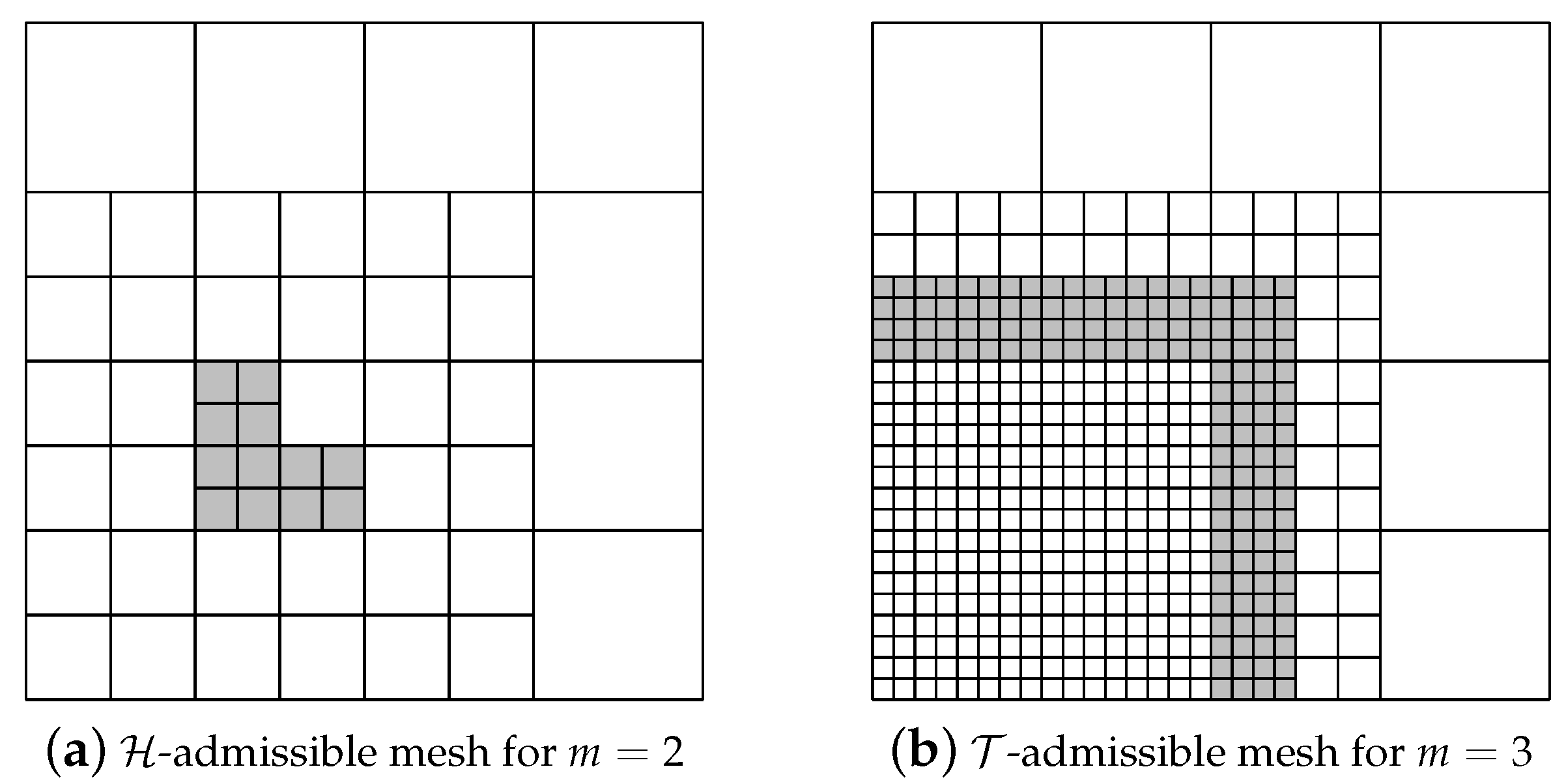
The definition of the auxiliary subdomains, and their role in strict admissibility, is better understood with the help of Figure 1. We represent and for different mesh configurations and degrees, and note that, in all cases , and the difference becomes bigger with higher degree. Moreover, in the examples of the figure, the subdomains and do not change between the top and bottom row, so also the auxiliary subdomains and do not change. Finally, for the degree and the class in the caption of each subfigure, we can refine the highlighted region (respectively, ), adding one more level and maintaining the strict -admissibility (resp. strict -admissibility) of the mesh.
The relation between the different admissibility classes is also stated in Proposition 1. One of the results of this proposition requires the following assumption:
This means that, for any mesh element Q, at least one B-spline of the same level of Q, whose support overlaps this element, is active in the hierarchical B-spline basis. The assumption may not be satisfied when refining few adjacent elements, as in the example of Figure 2 below.
Proposition 1.
Let be a hierarchical mesh. We have the following results:
- 1.
- if is strictly -admissible of class m, then it is -admissible of the class m.
- 2.
- if is strictly -admissible of class m, then it is -admissible of the class m.
- 3.
- if is (strictly) -admissible of class m, then it is (strictly) -admissible of the class m.
- 4.
- if is -admissible of class m and satisfies assumption (5), then it is strictly -admissible of the class m.
Proof.
Point 1 was already proved in [5] (Prop. 9). Point 3 is a trivial consequence of Definition 3 and the reduced support of THB-splines for admissible meshes, and a consequence of Definition 6 and the fact that for strictly admissible meshes. It remains to prove Points 2 and 4.
Given an active element , by definition of hierarchical B-splines, we know that any finer function in , with vanishing on Q. We need to prove that the same is true for any . Since , by definition of all the functions of level that do not vanish on Q have support contained in , and are not active. Noting that , for , we can use the same argument for coarser levels. This proves Point 2.
To prove Point 4, let the mesh element for . We observe that, under assumption (5), since the mesh is -admissible, the B-splines in whose support overlaps Q belong to levels . Consequently, it does not exist an active B-spline in of level whose support overlaps Q. The support extension of Q with respect to level is then completely contained in , and since this holds for any active element of level ℓ, we have , namely the mesh is strictly -admissible. ☐
Points 2 and 4 of Proposition 1 prove the equivalence of -admissibility and strictly -admissibility under assumption (5). In general, however, if the hierarchical mesh is -admissible (-admissible) of class m, then it is not necessarily strictly -admissible (respectively, -admissible). Counterexamples for both cases are shown in Figure 2, where we highlight the elements in , and thus, in , such that are not contained in . Notice that, in the -admissible mesh, the highlighted elements are precisely those that do not satisfy (5). In the -admissible case instead, the highlighted elements of level do not belong to for .
The last two algorithms of this section adapt to our setting the recursive refinement algorithm in [5], that, given an admissible hierarchical mesh and a set of marked elements, generates a refined -admissible mesh. Similar to the usage of cell-arrays in Octave/Matlab, we write when referring to the marked elements of all levels, and when referring to a single level.
The refinement algorithm is presented in Algorithm 5. Given a set of marked (active) elements, in lines 1 to 3, we first enrich this set by a recursive algorithm, explained in detail below, where all active elements in the neighborhood of the marked ones are also marked. Then, in line 4, we refine the hierarchical mesh by refining the updated set of marked elements, and replacing them with their children. This second step can be done as in [11] (Algorithm 2), and is not limited to dyadic refinement. After refining the hierarchical mesh, it is necessary to refine the hierarchical space, that is, to update the list of active basis functions. This last step, which we omit, has been already explained in [11].
| Algorithm 5: admissible_refinement. Description: given a hierarchical mesh and a set of marked elements, generate a refined admissible mesh of class m. |
Input:
|
Finally, Algorithm 6 is a recursive algorithm that, given a list of marked elements, adds the elements in their neighborhood (either or ) to the list. The difference between the two kinds of admissibility only affects the algorithm in the computation of the neighborhood (see Definition 5), in lines 1 to 5. Recursivity is necessary because, to guarantee admissibility, we must also mark the elements in the neighborhood of the newly marked ones.
As we mentioned above, our algorithm is a simple adaption of the one in [5] for -admissible meshes, while for -admissible meshes it generalizes to arbitrary the refinement algorithm in [7] (Algorithm 3.1), which only considers the case . Note that -admissible refinements for were also considered in [19].
| Algorithm 6: mark_recursive. Description: recursive algorithm to mark the elements in the neighborhood of marked ones. |
Input:
|
The properties of these algorithms were analyzed in [5] and [7,19], for (strictly) - and -admissibility, respectively. We report in Lemma 1 and Proposition 2 the proofs of the key results for Algorithm 5, which include both cases in a unified setting.
Lemma 1.
Let be a strictly -admissible (respectively, strictly -admissible) hierarchical mesh of class m, associated with a hierarchical space V, let a set of marked active elements, and let the integer . The call to Algorithm 5 in the form
terminates and returns a refined mesh , such that all elements in were already active, or are obtained by a single refinement of an element of .
Proof.
The algorithm terminates because the recursive algorithm ends when the neighborhood is empty, and this condition is reached in a finite number of steps (see lines 1 to 3 in Algorithms 3 and 4). The elements in the input set are all active in , and the neighborhood only consists of active elements in , hence the output set of mark_recursive (Algorithm 6) is a list of active elements in . Since no further marking is performed, all elements in were already active, or are obtained by a single refinement of an element in . ☐
Proposition 2.
Let , V, and m the input arguments of Algorithm 5, as in Lemma 1, where is strictly -admissible (respectively, strictly -admissible) of class m. Then, the algorithm returns a refined hierarchical mesh , which is strictly -admissible (resp. strictly -admissible) of class m.
Proof.
The proof follows the same steps for strictly -admissible and strictly -admissible meshes, so we will prove both at once, introducing the notation
and remarking any other important difference whenever needed.
Let us denote by , for , the subdomains after refinement. We use the same subindex () to identify whatever depends on the subdomains, such as the active elements at each level as in Equation (1), and the auxiliary subdomains .
Let , and we have by definition . We need to prove that (with the notation introduced above). There exist two possibilities, depending on whether was already active or not.
- If , then . Obviously, since for every k, it holds (both for - and -admissible), and we obtain the desired result.
- If , by Lemma 1, it is obtained by a single refinement of an element , thus . The definition of multilevel support extension immediately gives, for any ,Moreover, since is strictly admissible we know that , which combined with the previous equation and the definition of yieldsAccording to this, let us introduce for strictly -admissible meshes, and for strictly -admissible meshes. Since was a marked element (either , or it was marked during the recursive marking), it has been used as an input for mark_recursive (Algorithm 6), and as a consequence all the active elements in have been marked. Hence, , and by definition of the result is proved.
☐
Proposition 2 guarantees that the strictly admissible nature of the meshes is preserved by Algorithm 5 during the iterative marking and refinement processes of the adaptive loop. Several examples of strictly - and -admissible meshes obtained with this algorithm will be shown in Section 5.
Remark 1.
It is important to note that, since the two bases span the same hierarchical space, one could apply the strictly -admissible refinement with the standard HB-splines (or the strictly -admissible refinement with THB-splines). In general, the admissibility property is not valid for HB-splines on -admissible meshes, while it is always valid for THB-splines on -admissible meshes, as already stated in Proposition 1. The lack of the admissibility property has a negative impact on the sparsity of the matrix, as we will see in the numerical tests of the following section.
Remark 2.
The linear complexity of Algorithm 6 was proved in [20] for strictly -admissible meshes, and, subsequently, in [7] and [19] for strictly -admissible meshes of class and , respectively. The complexity estimates provide an upper bound for the number of elements generated by the adaptive strategy with respect to the number of elements marked for refinement. These results are in line with the estimates obtained in the context of adaptive finite element methods [21,22]. Note that the complexity analysis of the refinement algorithms is a fundamental ingredient to prove the optimality of hierarchical isogeometric methods [6,7].
4. Adaptive Isogeometric Methods
The hierarchical spaces are a natural choice for the definition of adaptive isogeometric methods [5,6,7], which are usually based on the adaptive loop
In order to illustrate the framework of such kind of methods, let us consider the Poisson model problem with Dirichlet boundary conditions
where is the physical domain, parametrized by the mapping .
To solve the model problem, we consider the hierarchical spline space , which gives the discretization space . Then, we determine the solution of the discretized problem (in its variational form)
where , with and a lifting of an approximation of the boundary function, such that , that we obtain by an -projection (see [16]). Note that (7) leads to a linear system whose structure depends on the choice of or as basis of V.
To estimate the error, and assuming that the basis functions are at least continuous, we employ the following element-based residual error estimator [5]. For any , the estimator is defined as
where . We note that other estimators, such as the function based residual estimator in [23], or recovery-based error estimators [24,25] could also be used. At each iteration of the adaptive loop, we compute the initial set of marked elements by applying Dörfler’s marking strategy [26] with the indicator (8). Finally, in order to get admissible meshes, we refine applying the Algorithms of Section 3.
Note that this framework can be easily extended to multipatch configurations with continuity. Let us assume that the physical domain is composed of several patches , each with its own parametrization , which overall give a parametrization. Defining a tensor-product space on each patch with the restrictions of having coinciding knot vectors and control points at the interfaces is enough to get a spline space [1].
Then, multipatch hierarchical spline spaces are obtained with the same construction presented in Section 2.1, simply by considering multipatch spline spaces as elements of the sequence , that is, we have a multipatch space for each level. The refinement algorithms described in Section 3 do not need any significant modification: only the support extensions, which determine the neighborhoods of the cells, are modified according to the different supports of the multipatch basis functions (see [11] (Section 3.4) and [27] for more details).
Since the basis functions are only across the interfaces, the element-based estimator must take into account the jump of the normal derivative, that is, for any , the estimator is
where denotes the interface between two patches, and is the unit normal vector to .
Remark 3.
The admissible refinement algorithm can be easily extended to a posteriori estimators based on functions. In this case, one would first mark the elements in the support of the marked functions (see Algorithms 1 and 10 in [11]), and then apply the recursive marking of Algorithm 5 before refining the mesh.
5. Numerical Results
In this section, we present some numerical examples to show the effectivity of the proposed algorithms, and to compare the different admissibility classes presented in the previous sections. The first numerical test consists of an ad hoc refinement of the unit square, while, in the second numerical test, we perform automatic adaptivity for a Poisson problem with singular solution.
5.1. Diagonal Refinement of the Unit Square
In the first numerical test, we study how the choice of the basis and the admissibility class may affect the matrix of the linear system arising in the isogeometric method. In particular, we are interested in the sparsity pattern and the condition numbers of the matrices.
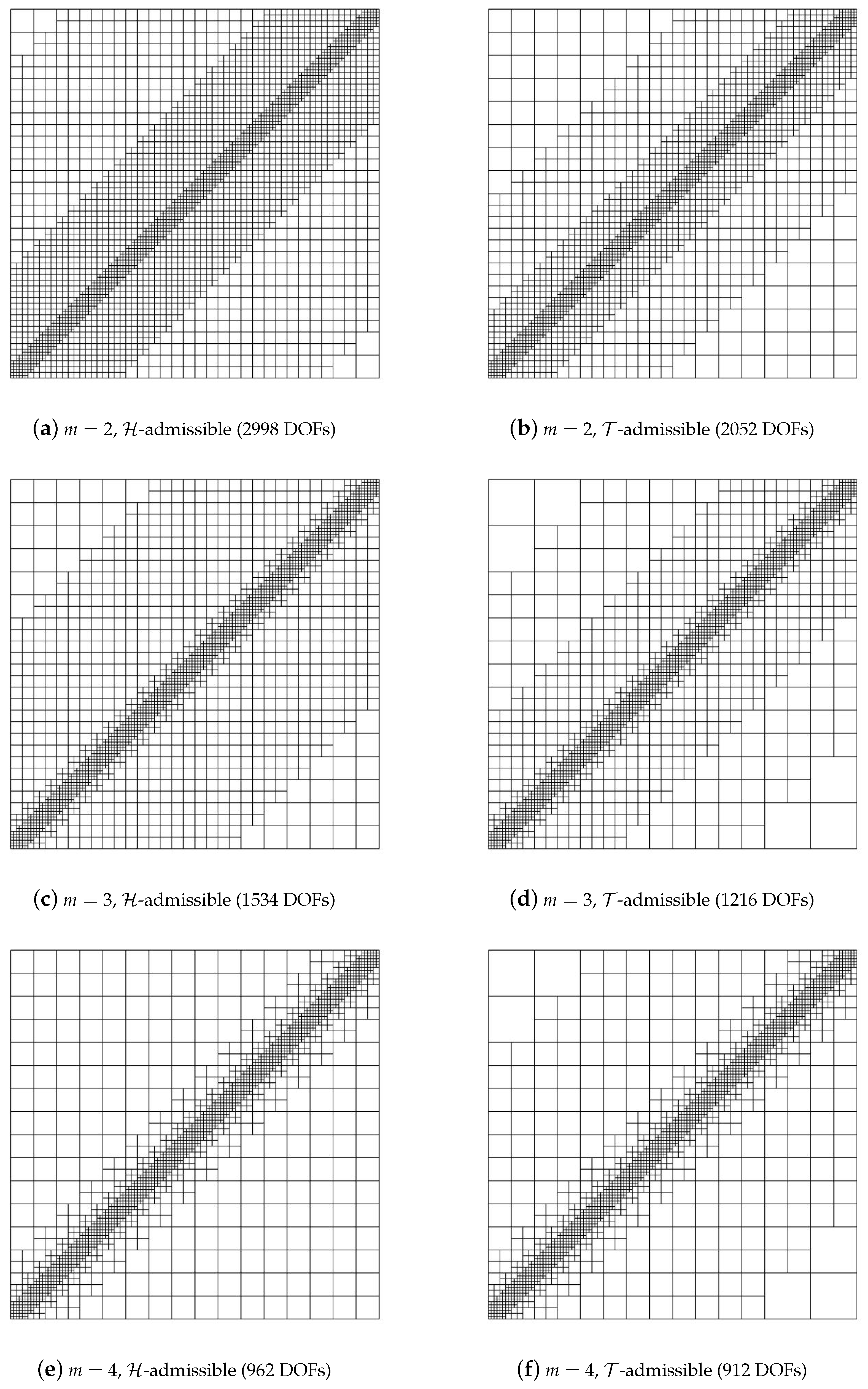
For our numerical tests, we have chosen a diagonal refinement of the unit square, similar to the one used in [13], as it gives a good compromise between locality of the refinement and an increasing number of basis functions at each step. More precisely, we start from a mesh, and at each step refine a strip of cells centered at the diagonal (compared to cells in [13]), which ensures that at each step we add functions of the finest level. The meshes obtained after six levels of refinement are shown in Figure 3, Figure 4 and Figure 5 for degrees two, three and four, respectively. The degrees of freedom (DOFs) associated to the different meshes are also indicated.
In Table 1, Table 2 and Table 3, we show the number of nonzeros of the stiffness matrix, and its percentage with respect to the global size of the matrix, after ten refinement steps, for HB-splines and THB-splines considering degrees , and for strictly -admissible and strictly -admissible hierarchical meshes of classes , where corresponds to refining only the marked elements of the finest level. The reduced support of THB-splines always reduces the number of nonzero entries compared to HB-splines, and this reduction is more evident for -admissible meshes and for high values of m. For -admissible meshes, instead, the reduction is not so significant, as the number of functions acting on one element is bounded for HB-splines. We also point out that higher values of m increase the number of nonzero entries with respect to the global size of the matrix, especially for high degree.
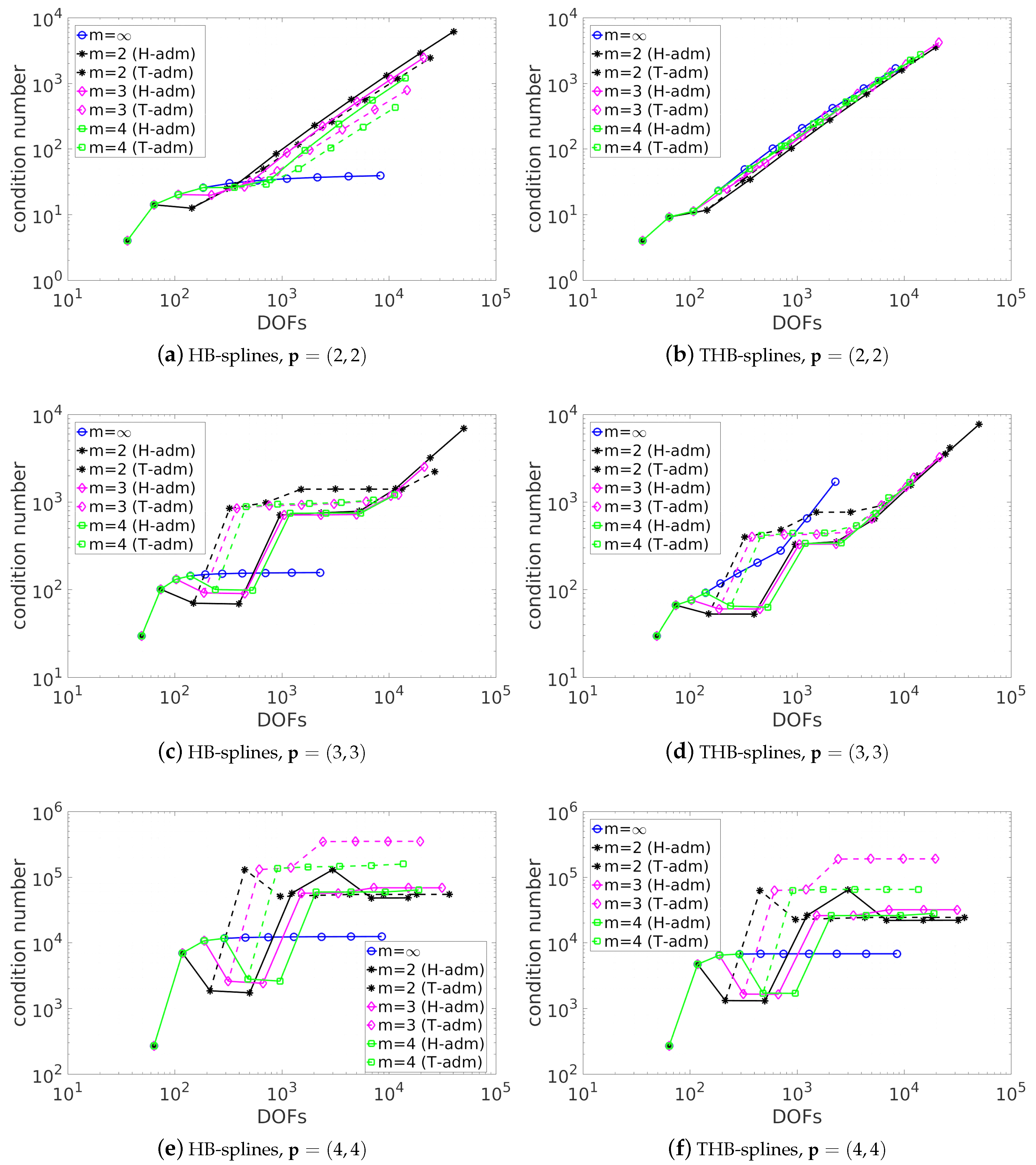
In Figure 6 and Figure 7, we show the computations of the condition number for the mass and the stiffness matrix, respectively, the latter computed after applying Dirichlet homogeneous boundary conditions. The results in Figure 6 show that, for the mass matrix, THB-splines get a lower condition number than HB-splines. Moreover, -admissible meshes give lower condition numbers than the corresponding -admissible ones, and lower values of m also produce lower condition numbers, which suggests that limiting the interaction between levels reduces the condition number of the mass matrix. These conclusions cannot be applied to the stiffness matrix. Indeed, the results of Figure 7 do not show any clear advantage of any option, neither for the chosen basis, nor for the admissibility class. We remark that for this particular refinement HB-splines in non-admissible meshes surprisingly provide the lowest condition numbers, which is completely opposite to the behavior for the mass matrix. It should be mentioned that a similar study for THB-splines defined on general (non admissible) hierarchical meshes and strictly admissible meshes of class 2 was already presented in [28]. In that case, there were some advantages on admissible meshes also for the condition number of the stiffness matrix. A better understanding of the problem would require a deeper investigation, which is behind the scope of the present paper.
5.2. Adaptive Method
For our second numerical test, we present the results obtained by applying the adaptive isogeometric methods described in Section 4 to the model problem (6) where and g is the restriction to of the exact solution
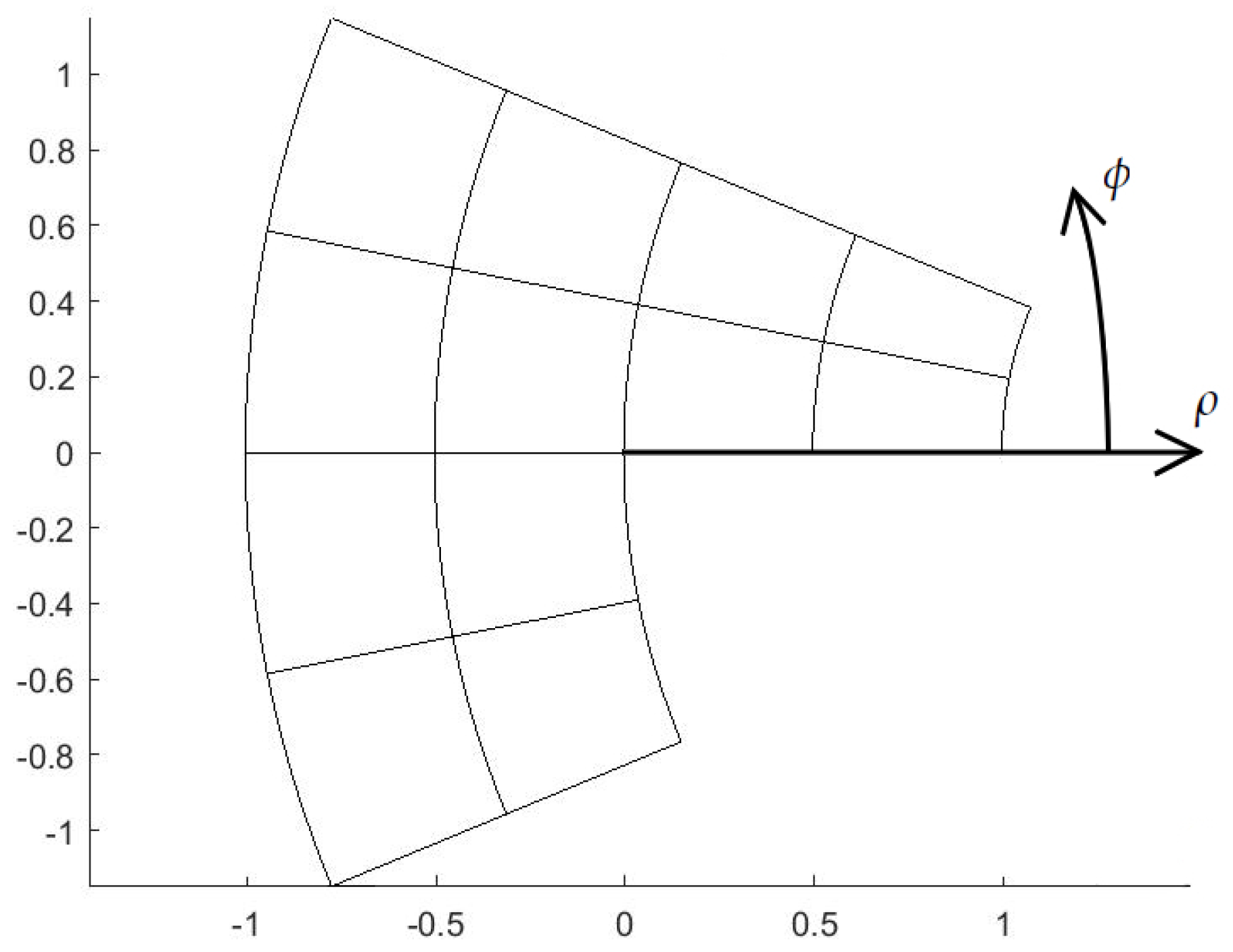
defined in polar coordinates on the curved L-shaped domain shown in Figure 8, which is formed by three patches.
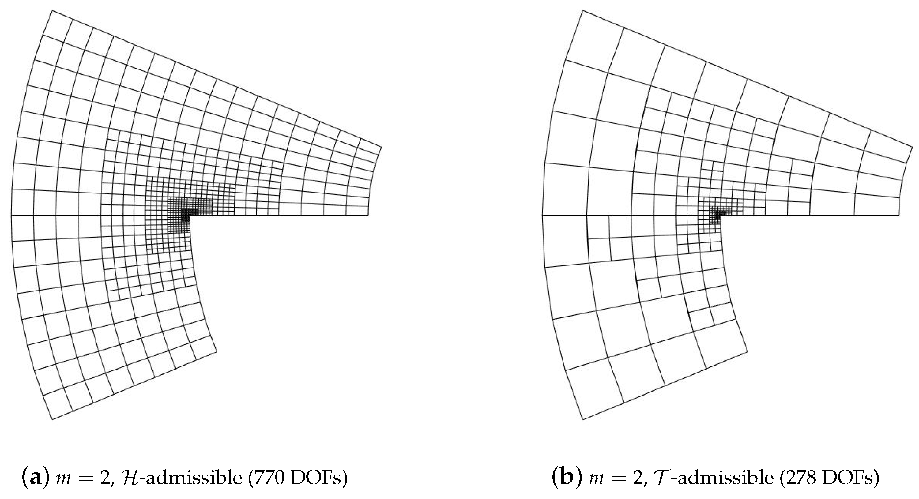
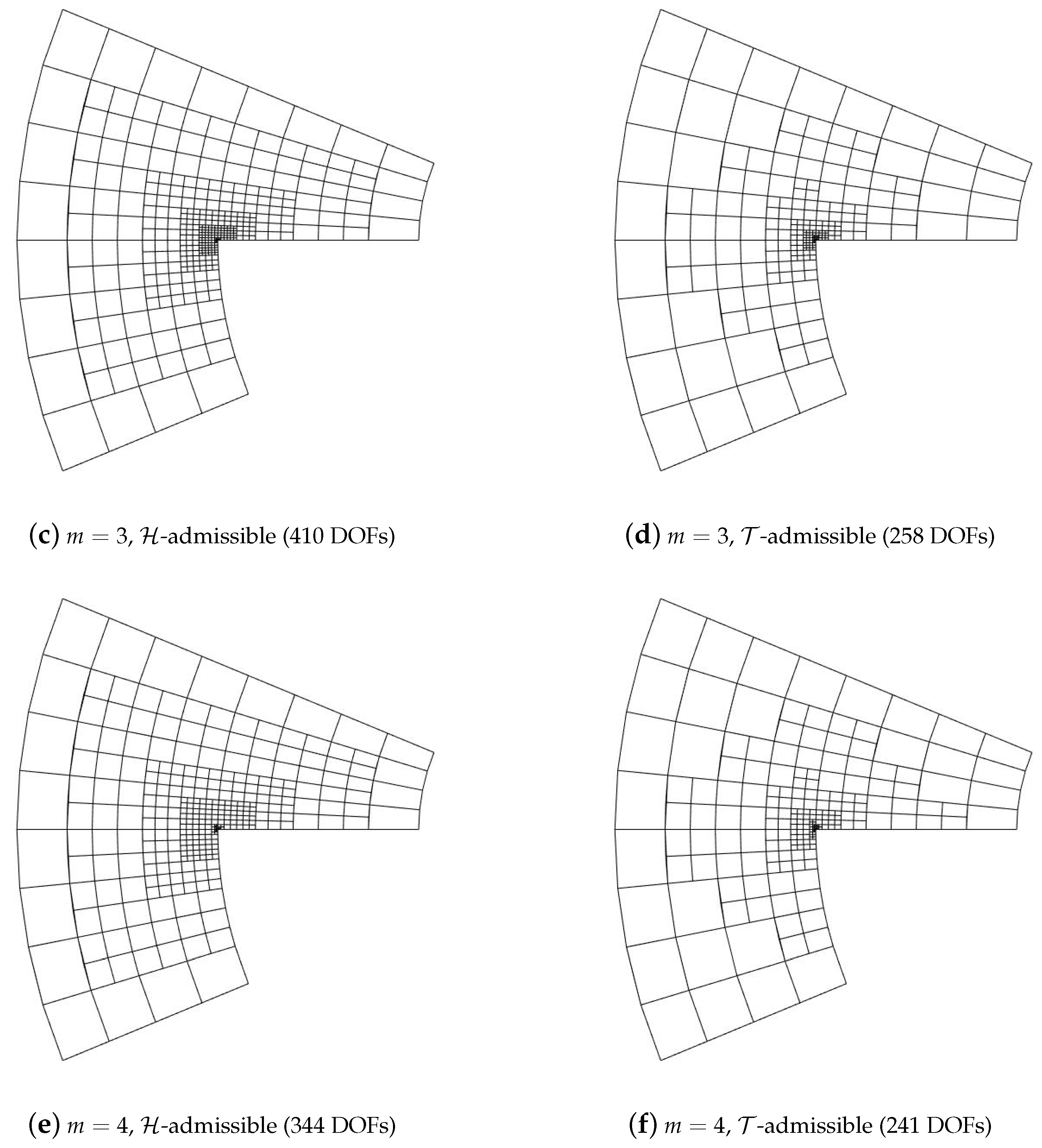
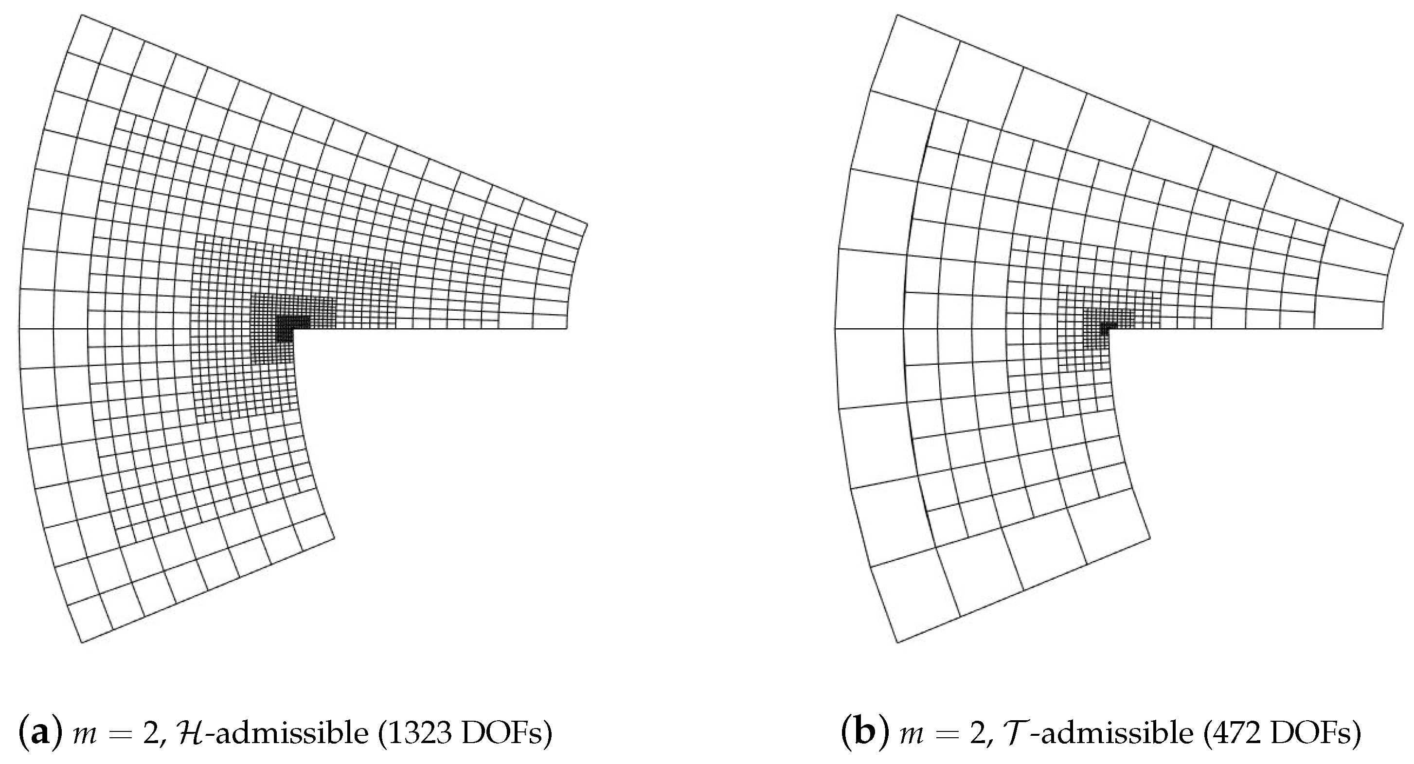
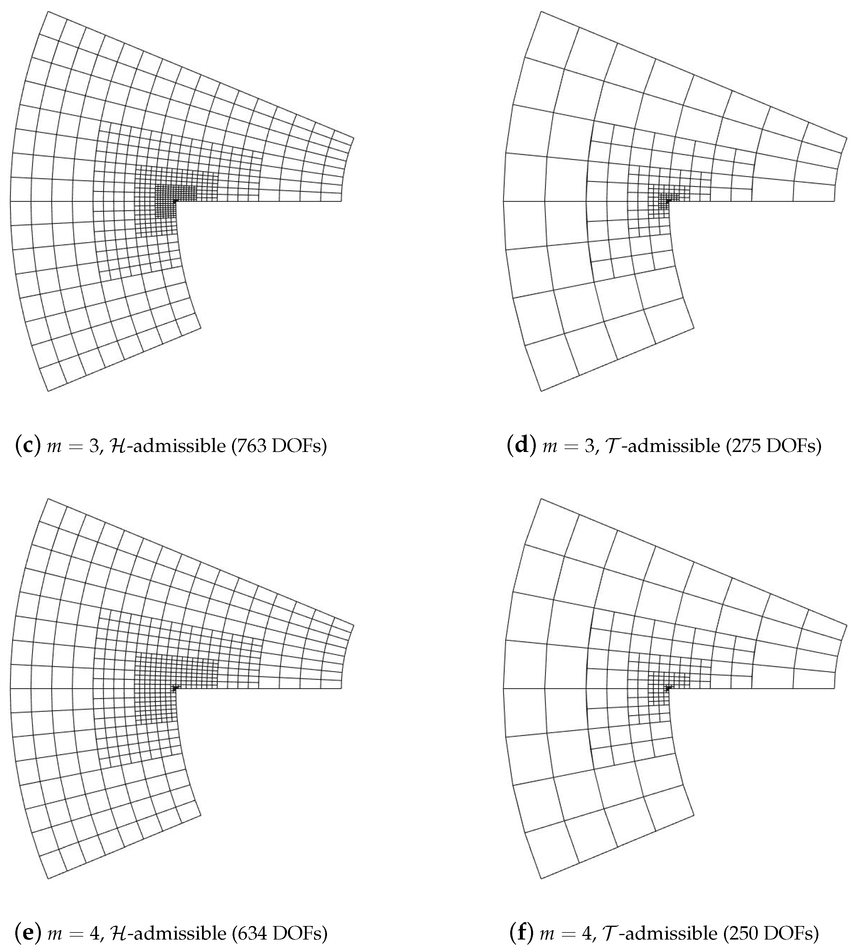
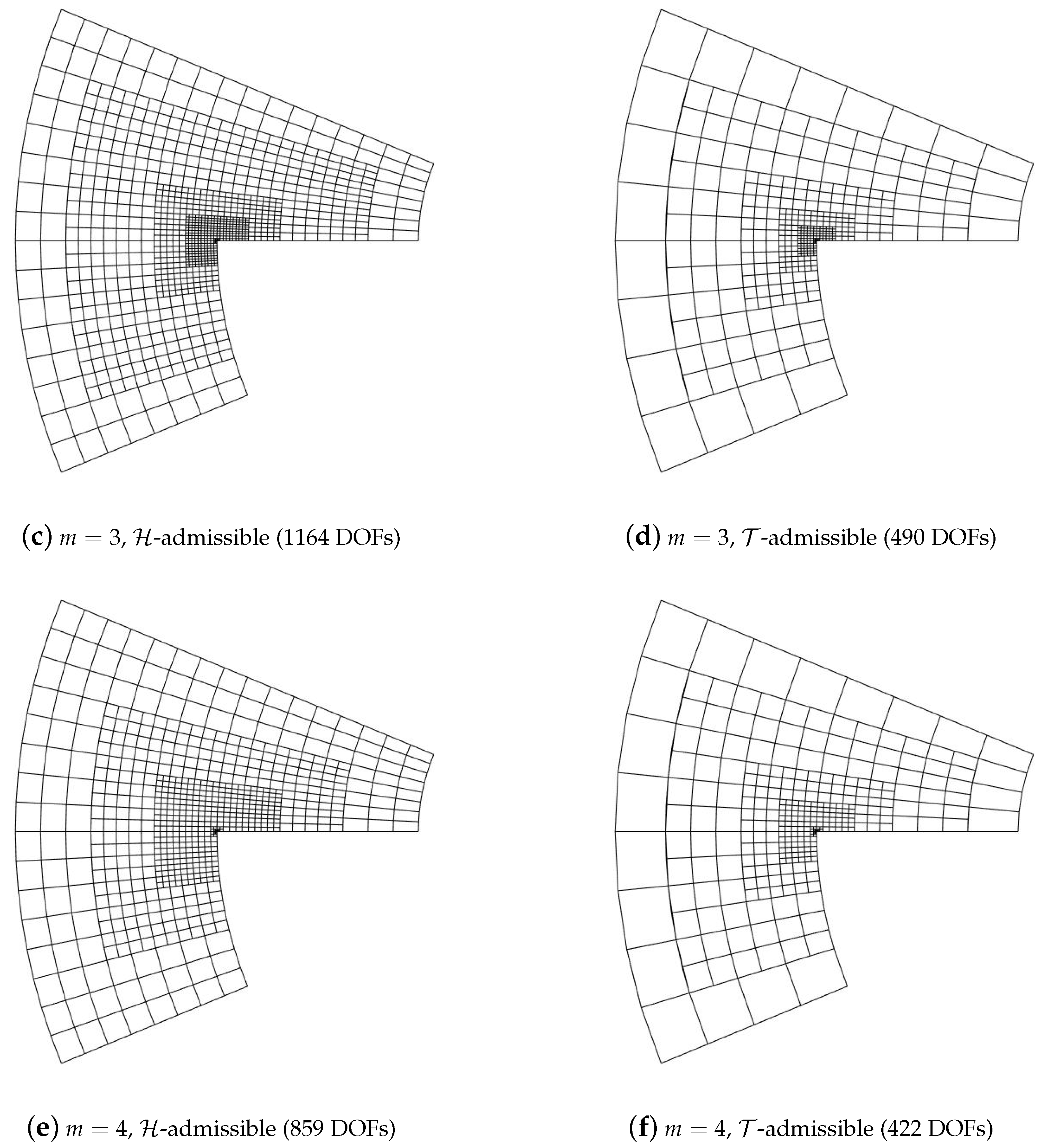
We apply the method with degrees and continuity inside each patch, and continuity across the interfaces, using classes of -admissibility and -admissibility , where corresponds to pure Dörfler’s marking, without later applying the recursive marking of Section 3. In all of the cases, the inital mesh is a 3-patch mesh with a mesh on each patch, and we set a limit of maximum hierarchical levels. For the Dörfler’s marking strategy, we set the value of the parameter . Figure 9, Figure 10 and Figure 11 show, for each degree and for each class of admissibility, the differences between -admissibility and -admissibility. These figures clearly show how the choice of the parameter m influences the grading of the mesh. As expected, -admissibility produces more refined meshes than -admissibility because the -neighborhood always contains the -neighborhood.
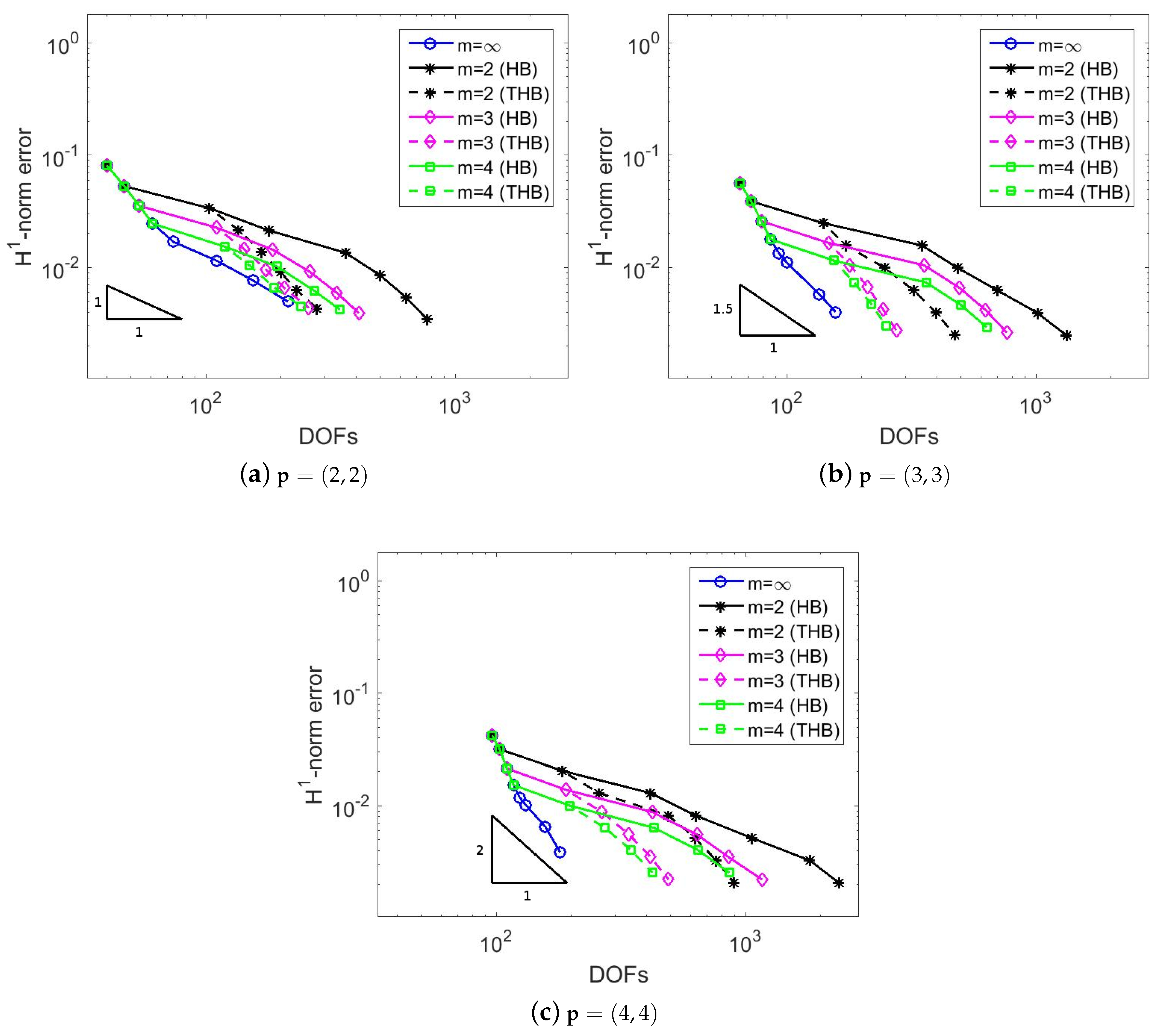
The importance of the admissibility class is more evident in Figure 12, where we show the convergence of the error in -norm with respect to the number of degrees of freedom. While both -admissible and -admissible meshes provide optimal convergence rates, the -admissible ones require a lower number of degrees of freedom to obtain the same error. This difference between the two classes is particularly evident for higher degree of the basis functions. Obviously, when no additional refinement is considered () the refinement is even more localized, but the assumptions of the current theory of adaptive isogeometric methods with hierarchical splines (see [5,6,7]) are not satisfied.
6. Conclusions
We presented a general framework for the design and implementation of refinement algorithms with (truncated) hierarchical B-splines. The properties of the admissible mesh configurations obtained with the iterative application of these algorithms were thoroughly analyzed. Note that the structure of hierarchical meshes with a certain class of admissibility can be naturally connected with a corresponding mesh grading, as confirmed by the numerical examples. The truncation mechanism behind the construction of THB-splines influences the strictly -admissible property leading to more localized refinement possibilities (and in turn to a reduced number of degrees of freedom) than the -admissible counterpart, that is, for the same admissibility class m. On the other hand, -admissible meshes guarantee a bounded number of hierarchical B-splines without the need of considering the truncated basis. The numerical examples also confirm the advantages of THB-splines with respect to the sparsity of the discretizations matrices and the condition number of the mass matrix. Concerning the condition number of the stiffness matrix, the situation is more unclear and a deeper study would be required. The comparison between - and -admissible refinements was never presented before and opens the path to additional studies on the optimal configuration for the development of hierarchical isogeometric methods.
The refinement algorithms here presented can be properly combined with coarsening algorithms that preserve the admissible nature of the mesh. This is an important aspect for controlling the effect of successive refinement and coarsening of hierarchical meshes in adaptive isogeometric methods (see e.g., [29,30]) and will be the subject matter of a future study.
Author Contributions
Conceptualization, C.B., C.G. and R.V.; Investigation, C.B., C.G. and R.V.; Methodology, C.B., C.G. and R.V.; Software, C.B., C.G. and R.V.; Writing—original draft, C.B., C.G. and R.V.; Writing—Review & Editing, C.B., C.G. and R.V.
Funding
This work was partially supported by the MIUR “Futuro in Ricerca” programme through the project “DREAMS”, grant number RBFR13FBI3. Rafael Vázquez has been partially supported by the ERC Advanced Grant “CHANGE”, grant number 694515, 2016-2020.
Acknowledgments
The authors are members of the INdAM Research group GNCS. The INdAM support through GNCS and Finanziamenti Premiali SUNRISE is gratefully acknowledged.
Conflicts of Interest
The authors declare no conflict of interest.
References
- Cottrell, J.A.; Hughes, T.J.R.; Bazilevs, Y. Isogeometric Analysis: Toward Integration of CAD and FEA; John Wiley & Sons: Hoboken, NJ, USA, 2009. [Google Scholar]
- Hughes, T.J.R.; Cottrell, J.A.; Bazilevs, Y. Isogeometric analysis: CAD, finite elements, NURBS, exact geometry and mesh refinement. Comput. Methods Appl. Mech. Eng. 2005, 194, 4135–4195. [Google Scholar] [CrossRef]
- Kraft, R. Adaptive and Linearly Independent Multilevel B-Splines. In Surface Fitting and Multiresolution Methods; Le Méhauté, A., Rabut, C., Schumaker, L.L., Eds.; Vanderbilt University Press: Nashville, TN, USA, 1997; pp. 209–218. [Google Scholar]
- Vuong, A.V.; Giannelli, C.; Jüttler, B.; Simeon, B. A hierarchical approach to adaptive local refinement in isogeometric analysis. Comput. Methods Appl. Mech. Eng. 2011, 200, 3554–3567. [Google Scholar] [CrossRef] [Green Version]
- Buffa, A.; Giannelli, C. Adaptive isogeometric methods with hierarchical splines: Error estimator and convergence. Math. Models Methods Appl. Sci. 2016, 26, 1–25. [Google Scholar] [CrossRef]
- Buffa, A.; Giannelli, C. Adaptive isogeometric methods with hierarchical splines: Optimality and convergence rates. Math. Models Methods Appl. Sci. 2017, 27, 2781–2802. [Google Scholar] [CrossRef]
- Gantner, G.; Haberlik, D.; Praetorius, D. Adaptive IGAFEM with optimal convergence rates: Hierarchical B-splines. Math. Models Methods Appl. Sci. 2017, 27, 2631–2674. [Google Scholar] [CrossRef] [Green Version]
- Giannelli, C.; Jüttler, B.; Speleers, H. THB-Splines: The truncated basis for hierarchical splines. Comput. Aided Geom. Des. 2012, 29, 485–498. [Google Scholar] [CrossRef]
- Bornemann, P.; Cirak, F. A subdivision-based implementation of the hierarchical B-spline finite element method. Comput. Methods Appl. Mech. Eng. 2013, 253, 584–598. [Google Scholar] [CrossRef]
- Scott, M.A.; Thomas, D.C.; Evans, E.J. Isogeometric spline forests. Comput. Methods Appl. Mech. Eng. 2014, 269, 222–264. [Google Scholar] [CrossRef]
- Garau, E.; Vázquez, R. Algorithms for the implementation of adaptive isogeometric methods using hierarchical B-splines. Appl. Numer. Math. 2018, 123, 58–87. [Google Scholar] [CrossRef]
- Kiss, G.; Giannelli, C.; Jüttler, B. Algorithms and data structures for truncated hierarchical B-splines. In Mathematical Methods for Curves and Surfaces; Floater, M., Lyche, T., Mazure, M.-L., Moerken, K., Schumaker, L.L., Eds.; Lecture Notes in Computer Science; Springer: Berlin/Heidelberg, Germany, 2014; Volume 8177, pp. 304–323. [Google Scholar]
- Giannelli, C.; Jüttler, B.; Kleiss, S.K.; Mantzaflaris, A.; Simeon, B.; Špeh, J. THB-splines: An effective mathematical technology for adaptive refinement in geometric design and isogeometric analysis. Comput. Methods Appl. Mech. Eng. 2016, 299, 337–365. [Google Scholar] [CrossRef]
- Hennig, P.; Müller, S.; Kästner, M. Bézier extraction and adaptive refinement of truncated hierarchical NURBS. Comput. Methods Appl. Mech. Eng. 2016, 305, 316–339. [Google Scholar] [CrossRef]
- D’Angella, D.; Kollmannsberger, S.; Rank, E.; Reali, A. Multi-level Bézier extraction for hierarchical local refinement of Isogeometric Analysis. Comput. Methods Appl. Mech. Eng. 2018, 328, 147–174. [Google Scholar] [CrossRef]
- Vázquez, R. A new design for the implementation of isogeometric analysis in Octave and Matlab: GeoPDEs 3.0. Comput. Math. Appl. 2016, 72, 523–554. [Google Scholar] [CrossRef]
- De Boor, C. A Practical Guide to Splines, revised ed.; Springer: Berlin/Heidelberg, Germany, 2001. [Google Scholar]
- Schumaker, L.L. Spline Functions: Basic Theory, 3rd ed.; Cambridge University Press: Cambridge, UK, 2007. [Google Scholar]
- Morgenstern, P. Mesh Refinement Strategies for the Adaptive Isogeometric Method. Ph.D. Thesis, Institut für Numerische Simulation, Rheinische Friedrich-Wilhelms-Universität Bonn, Bonn, Germany, 2017. [Google Scholar]
- Buffa, A.; Giannelli, C.; Morgenstern, P.; Peterseim, D. Complexity of hierarchical refinement for a class of admissible mesh configurations. Comput. Aided Geom. Des. 2016, 47, 83–92. [Google Scholar] [CrossRef] [Green Version]
- Binev, P.; Dahmen, W.; DeVore, R. Adaptive finite element methods with convergence rates. Numer. Math. 2004, 97, 219–268. [Google Scholar] [CrossRef]
- Stevenson, R. Optimality of a standard adaptive finite element method. Found. Comput. Math. 2007, 7, 245–269. [Google Scholar] [CrossRef]
- Buffa, A.; Garau, E.M. A posteriori error estimators for hierarchical B-spline discretizations. Math. Models Methods Appl. Sci. 2016. [Google Scholar] [CrossRef]
- Kumar, M.; Kvamsdal, T.; Johannessen, K.A. Superconvergent patch recovery and a posteriori error estimation technique in adaptive isogeometric analysis. Comput. Methods Appl. Mech. Eng. 2017, 316, 1086–1156. [Google Scholar] [CrossRef]
- Anitescu, C.; Hossain, M.N.; Rabczuk, T. Recovery-based error estimation and adaptivity using high-order splines over hierarchical T-meshes. Comput. Methods Appl. Mech. Eng. 2018, 328, 638–662. [Google Scholar] [CrossRef]
- Dörfler, W. A convergent algorithm for Poisson’s equation. SIAM J. Numer. Anal. 1996, 33, 1106–1124. [Google Scholar] [CrossRef]
- Buchegger, F.; Jüttler, B.; Mantzaflaris, A. Adaptively refined multi-patch B-splines with enhanced smoothness. Appl. Math. Comput. 2016, 272, 159–172. [Google Scholar] [CrossRef]
- Hennig, P.; Kästner, M.; Morgenstern, P.; Peterseim, D. Adaptive mesh refinement strategies in isogeometric analysis—A computational comparison. Comput. Methods Appl. Mech. Eng. 2017, 316, 424–448. [Google Scholar] [CrossRef]
- Lorenzo, G.; Scott, M.A.; Tew, K.; Hughes, T.J.R.; Gomez, H. Hierarchically refined and coarsened splines for moving interface problems, with particular application to phase-field models of prostate tumor growth. Comput. Methods Appl. Mech. Eng. 2017, 319, 515–548. [Google Scholar] [CrossRef]
- Hennig, P.; Ambati, M.; De Lorenzis, L.; Kästner, M. Projection and transfer operators in adaptive isogeometric analysis with hierarchical B-splines. Comput. Methods Appl. Mech. Eng. 2018, 334, 313–336. [Google Scholar] [CrossRef]
Figure 1.
The domains and are highlighted in dark gray and light gray, respectively, for different mesh configurations.
Figure 1.
The domains and are highlighted in dark gray and light gray, respectively, for different mesh configurations.
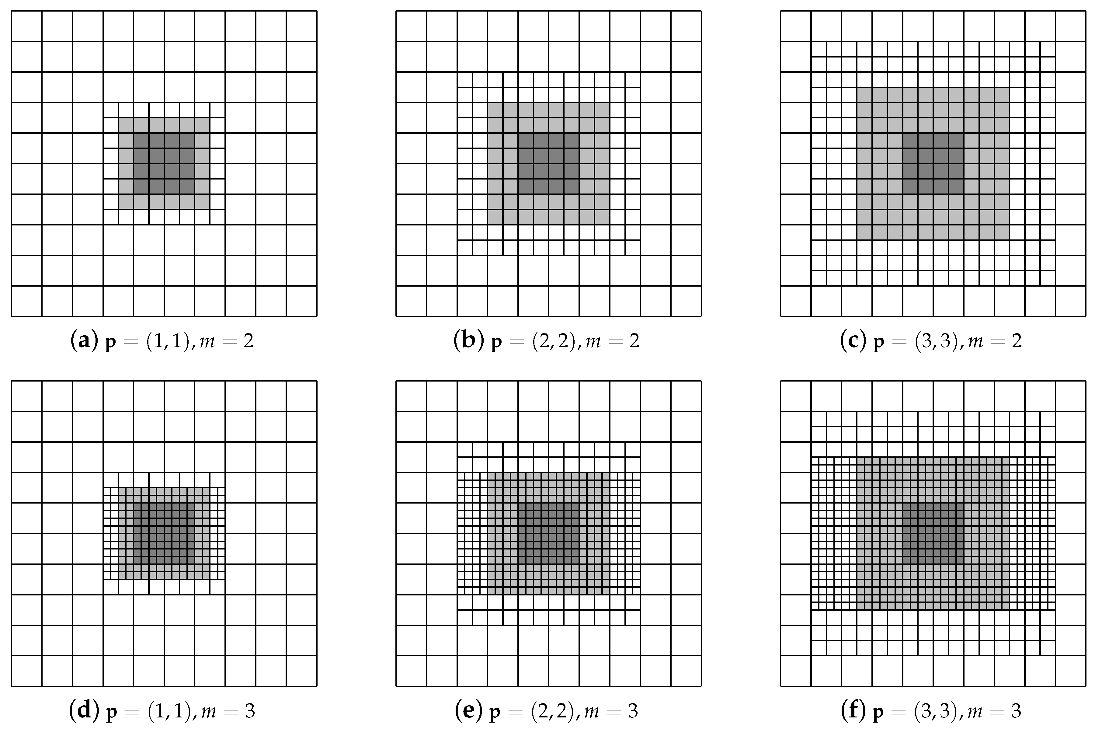
Figure 2.
Examples of degree of meshes that are admissible, but not strictly admissible.

Figure 3.
Hierarchical meshes obtained with and (from top to bottom), by using -admissible (left) and -admissible (right) meshes.
Figure 3.
Hierarchical meshes obtained with and (from top to bottom), by using -admissible (left) and -admissible (right) meshes.
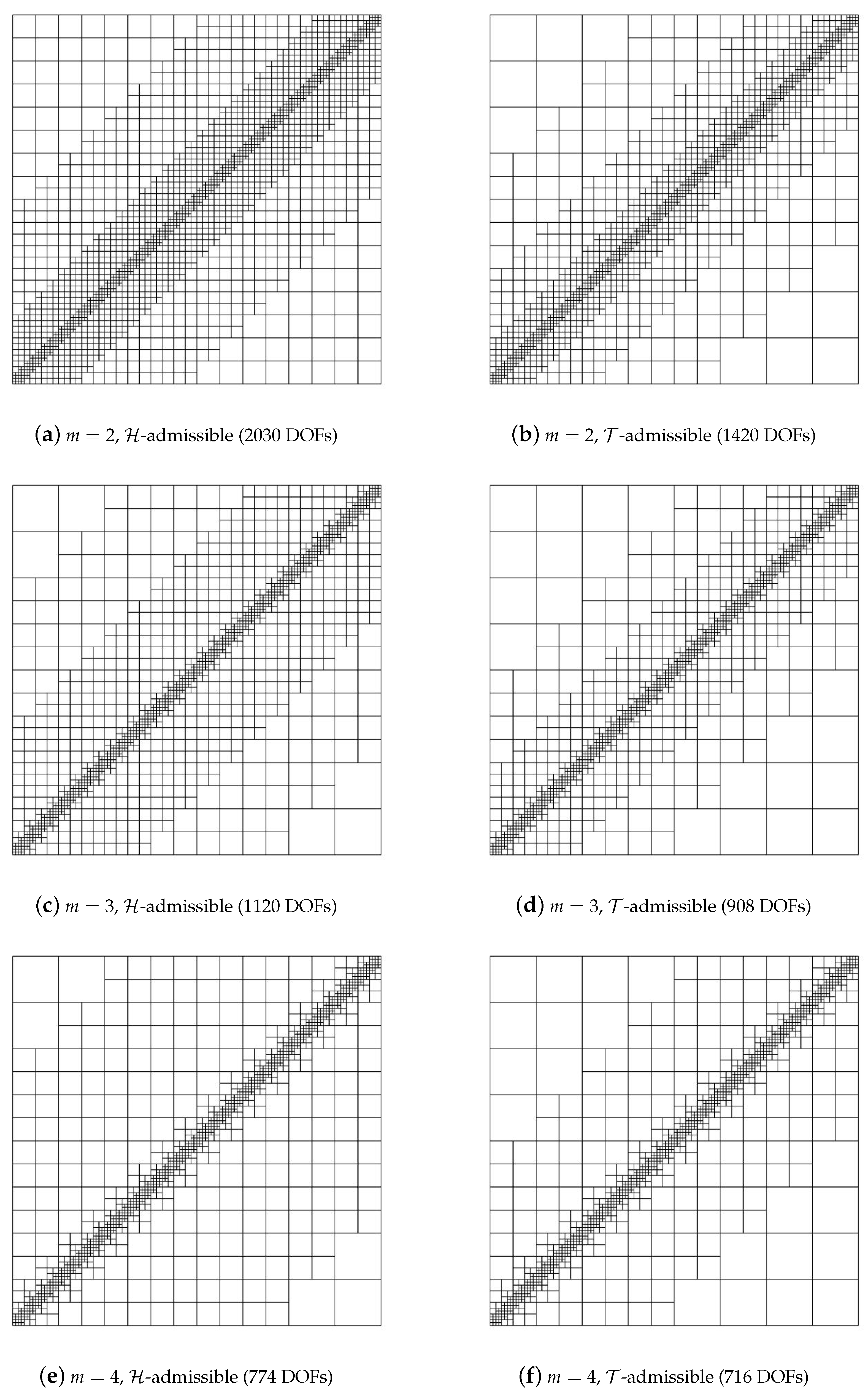
Figure 4.
Hierarchical meshes obtained with and (from top to bottom), by using -admissible (left) and -admissible (right) meshes.
Figure 4.
Hierarchical meshes obtained with and (from top to bottom), by using -admissible (left) and -admissible (right) meshes.
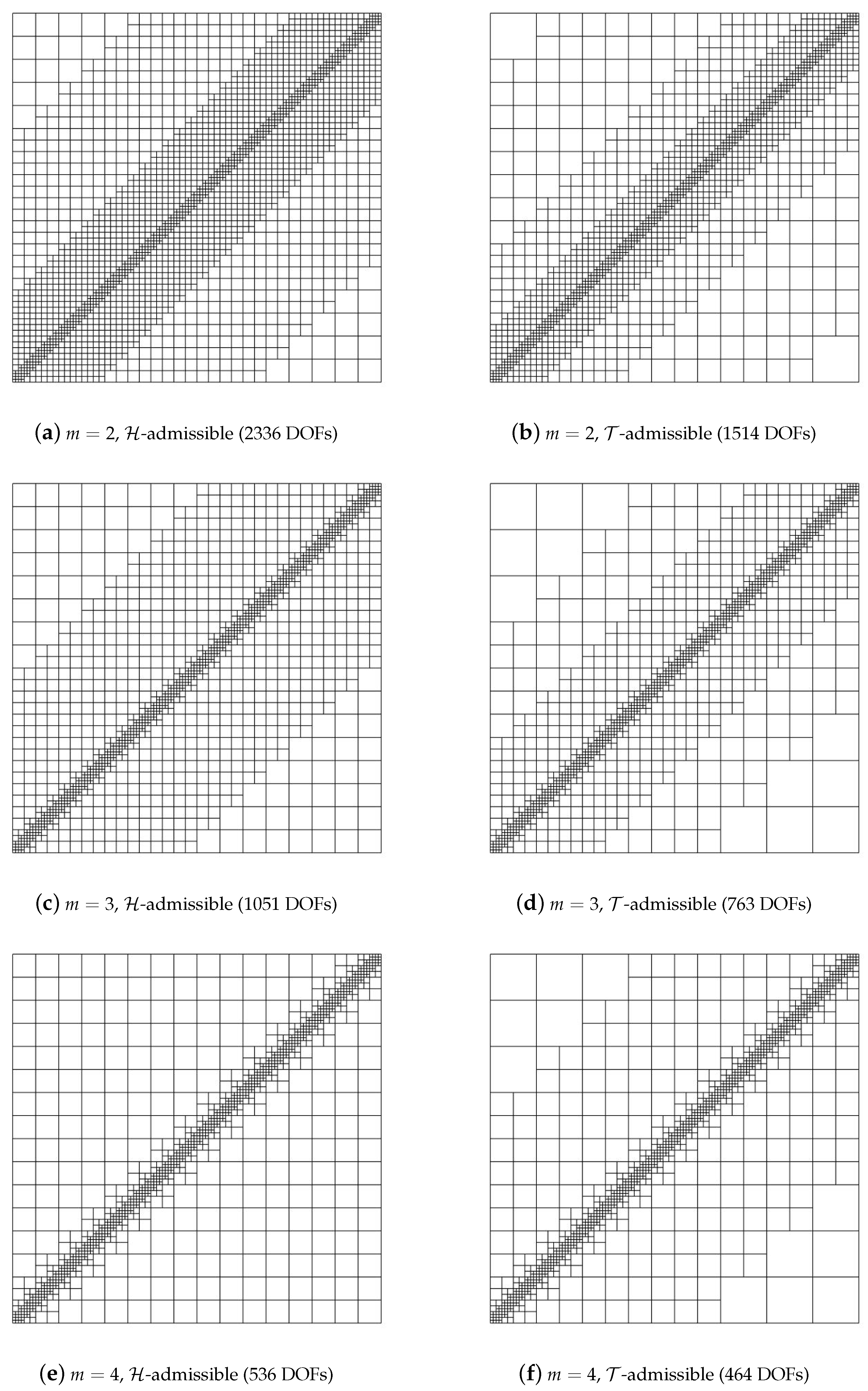
Figure 5.
Hierarchical meshes obtained with and (from top to bottom), by using -admissible (left) and -admissible (right) meshes.
Figure 5.
Hierarchical meshes obtained with and (from top to bottom), by using -admissible (left) and -admissible (right) meshes.

Figure 6.
Condition numbers of the mass matrix for HB-splines and THB-splines, for different admissibility classes and different values of the degree.
Figure 6.
Condition numbers of the mass matrix for HB-splines and THB-splines, for different admissibility classes and different values of the degree.
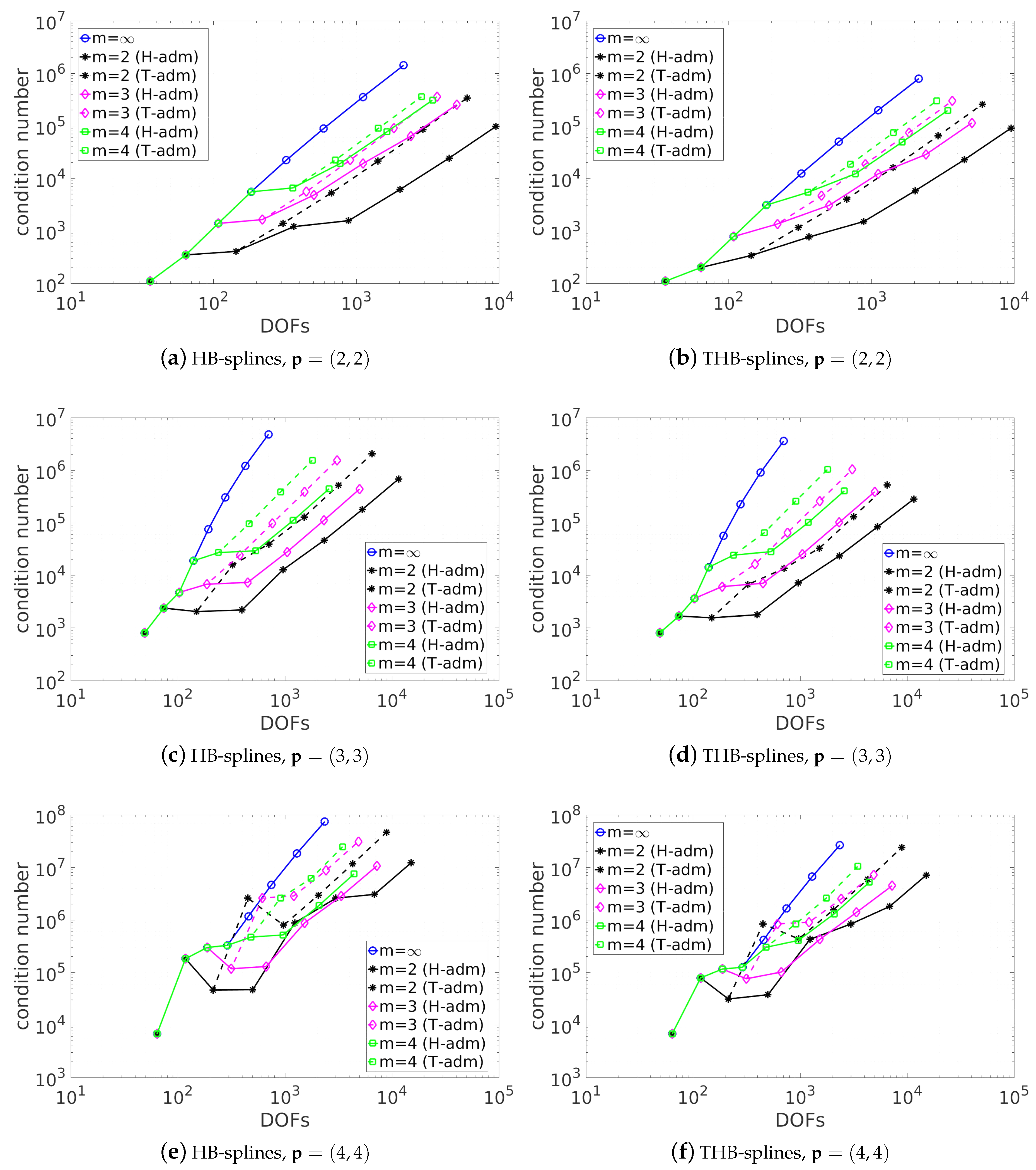
Figure 7.
Condition numbers of the stiffness matrix for HB-splines and THB-splines, for different admissibility classes and different values of the degree.
Figure 7.
Condition numbers of the stiffness matrix for HB-splines and THB-splines, for different admissibility classes and different values of the degree.

Figure 8.
Curved L-shaped domain with the initial mesh mapped on it.

Figure 9.
Hierarchical meshes obtained with and (from top to bottom), by using -admissible (left) and -admissible (right) meshes.
Figure 9.
Hierarchical meshes obtained with and (from top to bottom), by using -admissible (left) and -admissible (right) meshes.


Figure 10.
Hierarchical meshes obtained with and (from top to bottom), by using -admissible (left) and -admissible (right) meshes.
Figure 10.
Hierarchical meshes obtained with and (from top to bottom), by using -admissible (left) and -admissible (right) meshes.


Figure 11.
Hierarchical meshes obtained with and (from top to bottom), by using -admissible (left) and -admissible (right) meshes.
Figure 11.
Hierarchical meshes obtained with and (from top to bottom), by using -admissible (left) and -admissible (right) meshes.
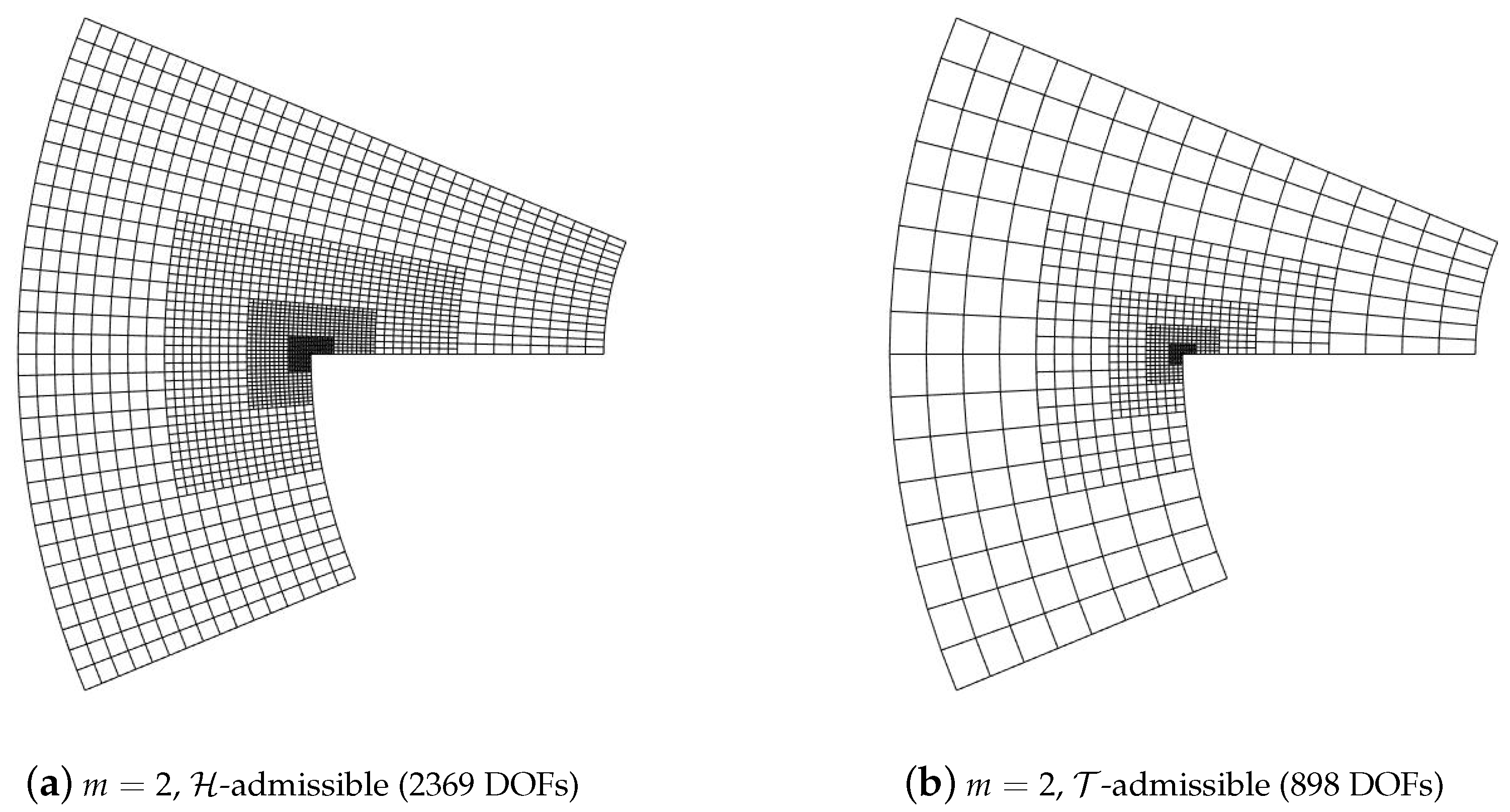

Figure 12.
Comparison of the convergence of the -norm error versus degrees of freedom (DOFs) for -admissible (HB) and -admissible (THB) meshes, with (from top to bottom).
Figure 12.
Comparison of the convergence of the -norm error versus degrees of freedom (DOFs) for -admissible (HB) and -admissible (THB) meshes, with (from top to bottom).


Table 1.
Number of nonzeros of the stiffness matrix for .
| DOFs | HB | (%) | THB | (%) | |||
|---|---|---|---|---|---|---|---|
| 8228 | 808,628 | (1.19) | 542,548 | (0.80) | |||
| -admissible | 40,058 | 1,248,786 | (0.08) | 1,099,583 | (0.07) | ||
| -admissible | 21,028 | 749,616 | (0.17) | 627,864 | (0.14) | ||
| -admissible | 14,106 | 589,834 | (0.30) | 476,115 | (0.24) | ||
| -admissible | 24,200 | 990,728 | (0.17) | 706,113 | (0.12) | ||
| -admissible | 14,664 | 898,652 | (0.42) | 478,963 | (0.22) | ||
| -admissible | 11,360 | 714,736 | (0.55) | 412,453 | (0.32) |
Table 2.
Number of nonzeros of the stiffness matrix for .
| DOFs | HB | (%) | THB | (%) | |||
|---|---|---|---|---|---|---|---|
| 2186 | 156,764 | (3.28) | 122,728 | (2.57) | |||
| -admissible | 49,940 | 2,941,926 | (0.12) | 2,620,770 | (0.11) | ||
| -admissible | 21,227 | 1,318,125 | (0.29) | 1,118,981 | (0.25) | ||
| -admissible | 11,064 | 674,020 | (0.55) | 571,544 | (0.47) | ||
| -admissible | 26,554 | 2,087,894 | (0.30) | 1,486,588 | (0.21) | ||
| -admissible | 12,107 | 1,466,741 | (1.00) | 709,261 | (0.48) | ||
| -admissible | 7020 | 746,362 | (1.51) | 392,128 | (0.80) |
Table 3.
Number of nonzeros of the stiffness matrix for .
| DOFs | HB | (%) | THB | (%) | |||
|---|---|---|---|---|---|---|---|
| 8446 | 1,819,856 | (2.55) | 1,410,796 | (1.98) | |||
| -admissible | 66,390 | 6,548,354 | (0.15) | 5,885,286 | (0.13) | ||
| -admissible | 31,112 | 3,299,540 | (0.34) | 2,861,116 | (0.30) | ||
| -admissible | 18,778 | 2,075,442 | (0.59) | 1,805,250 | (0.51) | ||
| -admissible | 36,516 | 4,819,354 | (0.36) | 3,499,152 | (0.26) | ||
| -admissible | 19,412 | 3,613,896 | (0.96) | 2,002,780 | (0.53) | ||
| -admissible | 13,456 | 2,773,686 | (1.53) | 1,437,096 | (0.79) |
© 2018 by the authors. Licensee MDPI, Basel, Switzerland. This article is an open access article distributed under the terms and conditions of the Creative Commons Attribution (CC BY) license (http://creativecommons.org/licenses/by/4.0/).
Share and Cite
MDPI and ACS Style
Bracco, C.; Giannelli, C.; Vázquez, R. Refinement Algorithms for Adaptive Isogeometric Methods with Hierarchical Splines. Axioms 2018, 7, 43. https://doi.org/10.3390/axioms7030043
AMA Style
Bracco C, Giannelli C, Vázquez R. Refinement Algorithms for Adaptive Isogeometric Methods with Hierarchical Splines. Axioms. 2018; 7(3):43. https://doi.org/10.3390/axioms7030043
Chicago/Turabian StyleBracco, Cesare, Carlotta Giannelli, and Rafael Vázquez. 2018. "Refinement Algorithms for Adaptive Isogeometric Methods with Hierarchical Splines" Axioms 7, no. 3: 43. https://doi.org/10.3390/axioms7030043
Note that from the first issue of 2016, this journal uses article numbers instead of page numbers. See further details here.