Neutrosophic Number Nonlinear Programming Problems and Their General Solution Methods under Neutrosophic Number Environments


Department of Electrical and Information Engineering, Shaoxing University, 508 Huancheng West Road, Shaoxing 312000, China
*
Author to whom correspondence should be addressed.
Axioms 2018, 7(1), 13; https://doi.org/10.3390/axioms7010013
Submission received: 22 January 2018
/
Revised: 16 February 2018
/
Accepted: 22 February 2018
/
Published: 24 February 2018
(This article belongs to the Special Issue Neutrosophic Multi-Criteria Decision Making)
Abstract
:In practical situations, we often have to handle programming problems involving indeterminate information. Building on the concepts of indeterminacy I and neutrosophic number (NN) (z = p + qI for p, q ∈ ℝ), this paper introduces some basic operations of NNs and concepts of NN nonlinear functions and inequalities. These functions and/or inequalities contain indeterminacy I and naturally lead to a formulation of NN nonlinear programming (NN-NP). These techniques include NN nonlinear optimization models for unconstrained and constrained problems and their general solution methods. Additionally, numerical examples are provided to show the effectiveness of the proposed NN-NP methods. It is obvious that the NN-NP problems usually yield NN optimal solutions, but not always. The possible optimal ranges of the decision variables and NN objective function are indicated when the indeterminacy I is considered for possible interval ranges in real situations.
1. Introduction
Traditional mathematical programming usually handles optimization problems involving deterministic objective functions and/or constrained functions. However, uncertainty also exists in real problems. Hence, many researchers have proposed uncertain optimization methods, such as approaches using fuzzy and stochastic logics, interval numbers, or uncertain variables [1,2,3,4,5,6]. Uncertain programming has been widely applied in engineering, management, and design problems. In existing uncertain programming methods, however, the objective functions or constrained functions are usually transformed into a deterministic or crisp programming problem to yield the optimal feasible crisp solution of the decision variables and the optimal crisp value of the objective function. Hence, existing uncertain linear or nonlinear programming methods are not really meaningful indeterminate methods because they only obtain optimal crisp solutions rather than indeterminate solutions necessary for real situations. However, indeterminate programming problems may also yield an indeterminate optimal solution for the decision variables and the indeterminate optimal value of the objective function suitable for real problems with indeterminate environments. Hence, it is necessary to understand how to handle indeterminate programming problems with indeterminate solutions.
Since there exists indeterminacy in the real world, Smarandache [7,8,9] first introduced a concept of indeterminacy—which is denoted by I, the imaginary value—and then he presented a neutrosophic number (NN) z = p + qI for p, q ∈ ℝ (ℝ is all real numbers) by combining the determinate part p with the indeterminate part qI. It is obvious that this is a useful mathematical concept for describing incomplete and indeterminate information. After their introduction, NNs were applied to decision-making [10,11] and fault diagnosis [12,13] under indeterminate environments.
In 2015, Smarandache [14] introduced a neutrosophic function (i.e., interval function or thick function), neutrosophic precalculus, and neutrosophic calculus to handle more indeterminate problems. He defined a neutrosophic thick function g: ℝ → G(ℝ) (G(ℝ) is the set of all interval functions) as the form of an interval function g(x) = [g1(x), g2(x)]. After that, Ye et al. [15] introduced the neutrosophic functions in expressions for the joint roughness coefficient and the shear strength in the mechanics of rocks. Further, Ye [16] and Chen et al. [17,18] presented expressions and analyses of the joint roughness coefficient using NNs. Ye [19] proposed the use of neutrosophic linear equations and their solution methods in traffic flow problems with NN information.
Recently, NNs have been extended to linguistic expressions. For instance, Ye [20] proposed neutrosophic linguistic numbers and their aggregation operators for multiple attribute group decision-making. Further, Ye [21] presented hesitant neutrosophic linguistic numbers—based on both the neutrosophic linguistic numbers and the concept of hesitant fuzzy logic—calculated their expected value and similarity measure, and applied them to multiple attribute decision-making. Additionally, Fang and Ye [22] introduced linguistic NNs based on both the neutrosophic linguistic number and the neutrosophic set concept, and some aggregation operators of linguistic NNs for multiple attribute group decision-making.
In practical problems, the information obtained by decision makers or experts may be imprecise, uncertain, and indeterminate because of a lack of data, time pressures, measurement errors, or the decision makers’ limited attention and knowledge. In these cases, we often have to solve programming problems involving indeterminate information (indeterminacy I). However, the neutrosophic functions introduced in [14,15] do not contain information about the indeterminacy I and also cannot express functions involving indeterminacy I. Thus, it is important to define NN functions containing indeterminacy I based on the concept of NNs, in order to handle programming problems under indeterminate environments. Jiang and Ye [23] and Ye [24] proposed NN linear and nonlinear programming models and their preliminary solution methods, but they only handled some simple/specified NN optimization problems and did not propose effective solution methods for complex NN optimization problems. To overcome this insufficiency, this paper first introduces some operations of NNs and concepts of NN linear and nonlinear functions and inequalities, which contain indeterminacy I. Then, various NN nonlinear programming (NN-NP) models and their general solution methods are proposed in order to obtain NN/indeterminate optimal solutions.
The rest of this paper is structured as follows. On the basis of some basic concept of NNs, Section 2 introduces some basic operations of NNs and concepts of NN linear and nonlinear functions and inequalities with indeterminacy I. Section 3 presents NN-NP problems, including NN nonlinear optimization models with unconstrained and constrained problems. In Section 4, general solution methods are introduced for various NN-NP problems, and then numerical examples are provided to illustrate the effectiveness of the proposed NN-NP methods. Section 5 contains some conclusions and future research.
2. Neutrosophic Numbers and Neutrosophic Number Functions
Smarandache [7,8,9] first introduced an NN, denoted by z = p + qI for p, q ∈ ℝ, consisting of a determinate part p and an indeterminate part qI, where I is the indeterminacy. Clearly, it can express determinate information and indeterminate information as in real world situations. For example, consider the NN z = 5 + 3I for I ∈ [0, 0.3], which is equivalent to z ∈ [5, 5.9]. This indicates that the determinate part of z is 5, the indeterminate part is 3I, and the interval of possible values for the number z is [5, 5.9]. If I ∈ [0.1, 0.2] is considered as a possible interval range of indeterminacy I, then the possible value of z is within the interval [5.3, 5.6]. For another example, the fraction 7/15 is within the interval [0.46, 0.47], which is represented as the neutrosophic number z = 0.46 + 0.01I for I ∈ [0, 1]. The NN z indicates that the determinate value is 0.46, the indeterminate value is 0.01I, and the possible value is within the interval [0.46, 0.47].
It is obvious that an NN z = p + qI may be considered as the possible interval range (changeable interval number) z = [p + q·inf{I}, p + q·sup{I}] for p, q ∈ ℝ and I ∈ [inf{I}, sup{I}]. For convenience, z is denoted by z = [p + qIL, p + qIU] for z ∈ Z (Z is the set of all NNs) and I ∈ [IL, IU] for short. In special cases, z can be expressed as the determinate part z = p if qI = 0 for the best case, and, also, z can be expressed as the indeterminate part z = qI if p = 0 for the worst case.
Let two NNs be z1 = p1 + q1I and z2 = p2 + q2I for z1, z2 ∈ Z, then their basic operational laws for I ∈ [IL, IU] are defined as follows [23,24]:
- (1)
- ;
- (2)
- ;
- (3)
- ;
- (4)
- .
For a function containing indeterminacy I, we can define an NN function (indeterminate function) in n variables (unknowns) as F(x, I): Zn → Z for x = [x1, x2, …, xn]T ∈ Zn and I ∈ [IL, IU], which is either an NN linear or an NN nonlinear function. For example, for x = [x1, x2]T ∈ Z2 and I ∈ [IL, IU] is an NN linear function, and for x = [x1, x2]T ∈ Z2 and I ∈ [IL, IU] is an NN nonlinear function.
For an NN function in n variables (unknowns) g(x, I): Zn → Z, we can define an NN inequality g(x, I) ≤ (≥) 0 for x = [x1, x2, …, xn]T ∈ Zn and I ∈ [IL, IU], where g(x, I) is either an NN linear function or an NN nonlinear function. For example, and for x = [x1, x2]T ∈ Z2 and I ∈ [IL, IU] are NN linear and NN nonlinear inequalities in two variables, respectively.
Generally, the values of x, F(x, I), and g(x, I) are NNs (usually but not always). In this study, we mainly research on NN-NP problems and their general solution methods.
3. Neutrosophic Number Nonlinear Programming Problems
An NN-NP problem is similar to a traditional nonlinear programming problem, which is composed of an objective function, general constraints, and decision variables. The difference is that an NN-NP problem includes at least one NN nonlinear function, which could be the objective function, or some or all of the constraints. In the real world, many real problems are inherently nonlinear and indeterminate. Hence, various NN optimization models need to be established to handle different NN-NP problems.
In general, NN-NP problems in n decision variables can be expressed by the following NN mathematical models:
- (1)
- Unconstrained NN optimization model:where x = [x1, x2, …, xn]T ∈ Zn, F(x, I): Zn → Z, and I ∈ [IL, IU].min F(x, I), x ∈ Zn,
- (2)
- Constrained NN optimization model:where g1(x, I), g2(x, I), …, gm(x, I), h1(x, I), h2(x, I), …, hl(x, I): Zn → Z, and I ∈ [IL, IU].min F(x, I)
s.t. gi(x, I) ≤ 0, I = 1, 2, …, m
hj(x, I) = 0, j = 1, 2, …, l
x ∈ Zn,
In special cases, if the NN-NP problem only contains the restrictions hj(x, I) = 0 without inequality constraints, gi(x, I) ≤ 0, then the NN-NP problem is called the NN-NP problem with equality constraints. If the NN-NP problem only contains the restrictions gi(x, I) ≤ 0, without constraints hj(x, I) = 0, then the NN-NP problem is called the NN-NP problem with inequality constraints. Finally, if the NN-NP problem does not contain either restrictions, hj(x, I) = 0 or gi(x, I) ≤ 0, then the constrained NN-NP problem is reduced to the unconstrained NN-NP problem.
The NN optimal solution for the decision variables is feasible in an NN-NP problem if it satisfies all of the constraints. Usually, the optimal solution for the decision variables and the value of the NN objective function are NNs, but not always). When the indeterminacy I is considered as a possible interval range (possible interval number), the optimal solution of all feasible intervals forms the feasible region or feasible set for x and I ∈ [IL, IU]. In this case, the value of the NN objective function is an optimal possible interval (NN) for F(x, I).
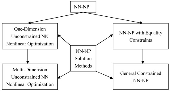
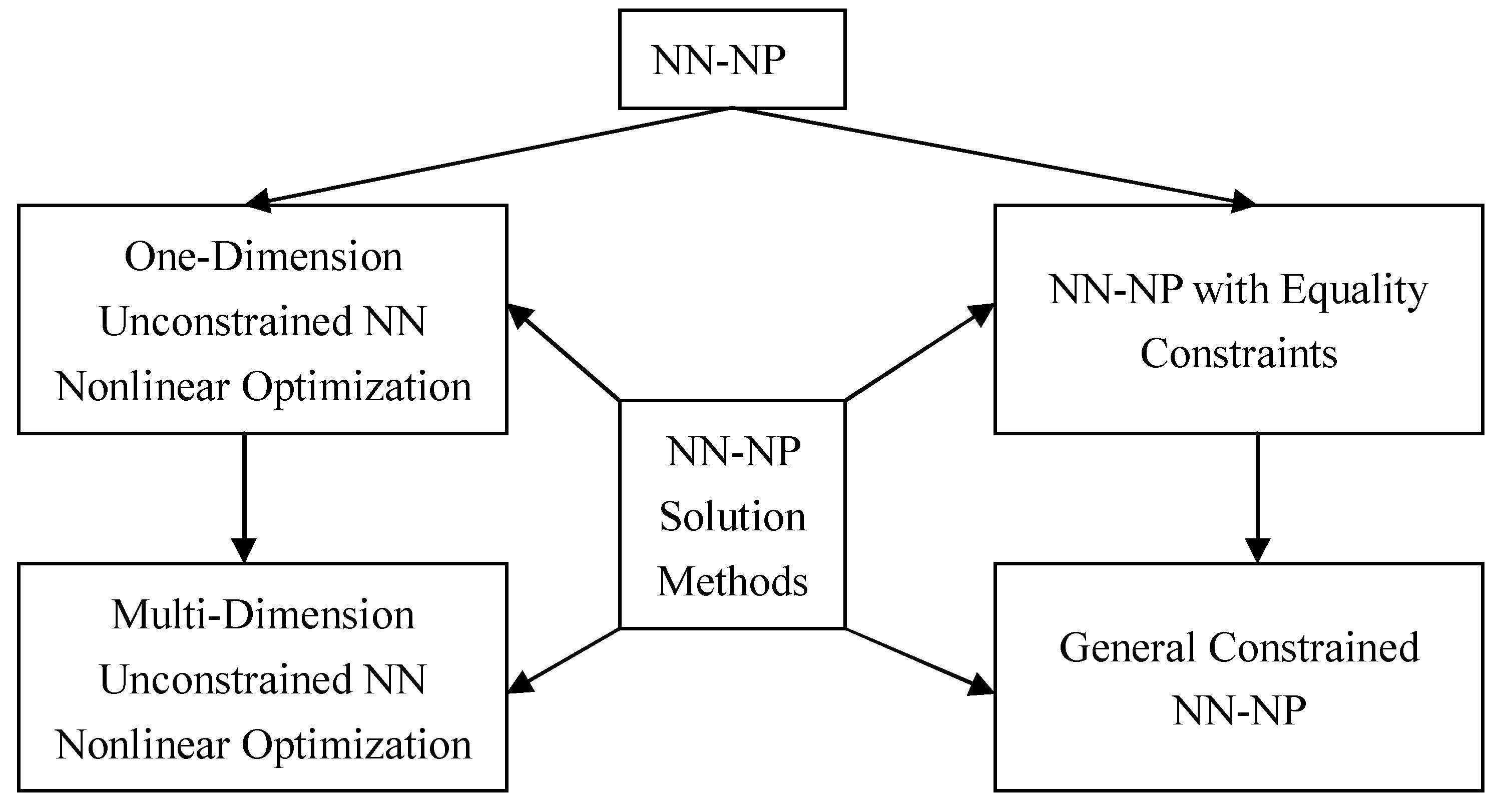
In the following section, we shall introduce general solution methods for NN-NP problems, including unconstrained NN and constrained NN nonlinear optimizations, based on methods of traditional nonlinear programming problems.
4. General Solution Methods for NN-NP Problems
4.1. One-Dimension Unconstrained NN Nonlinear Optimization
The simplest NN nonlinear optimization only has a nonlinear NN objective function with one variable and no constraints. Let us consider a single variable NN nonlinear objective function F(x, I) for x ∈ Z and I ∈ [IL, IU]. Then, for a differentiable NN nonlinear objective function F(x, I), a local optimal solution x* satisfies the following two conditions:
- (1)
- Necessary condition: The derivative is dF(x*, I)/dx = 0 for I ∈ [IL, IU];
- (2)
- Sufficient condition: If the second derivative is d2F(x*, I)/dx2 < 0 for I ∈ [IL, IU], then x* is an optimal solution for the maximum F(x*, I); if the second derivative is d2F(x*, I)/dx2 > 0, then x* is an optimal solution for the minimum F(x*, I).
Example 1.
An NN nonlinear objective function with one variable is F(x, I) = 2Ix2 + 5I for x ∈ Z and I ∈ [IL, IU]. Based on the optimal conditions, we can obtain:
Assume that we consider a specific possible range of I ∈ [IL, IU] according to real situations or actual requirements, then we can discuss its optimal possible value. If I ∈ [1, 2] is considered as a possible interval range, then d2F(x*, I)/dx2 > 0, and x* = 0 is the optimal solution for the minimum F(x*, I). Thus, the minimum value of the NN objective function is F(x*, I) = [5, 10], which, in this case, is a possible interval range, but not always. Specifically if I = 1 (crisp value), then F(x*, I) = 5.
4.2. Multi-Dimension Unconstrained NN Nonlinear Optimization
Assume that a multiple variable NN function F(x, I) for x = [x1, x2, …, xn]T ∈ Zn and I ∈ [IL, IU] is considered as an unconstrained differentiable NN nonlinear objective function in n variables. Then, we can obtain the partial derivatives:
Further, the partial second derivatives, structured as the Hessian matrix H(x, I), are:
Then, the Hessian matrix H(x, I) is structured as its subsets Hi(x, I) (i = 1, 2, …, n), where Hi(x, I) indicate the subset created by taking the first i rows and columns of H(x, I). You calculate the determinant of each of the n subsets at x*:
from the sign patterns of the determinates of Hi(x*, I) (i = 1, 2, …, n) for I ∈ [IL, IU], as follows:
- (1)
- If Hi(x*, I) > 0, then H(x*, I) is positive definite at x*;
- (2)
- If Hi(x*, I) < 0 and the remaining Hi(x*, I) alternate in sign, then H(x*, I) is negative definite at x*;
- (3)
- If some of the values which are supposed to be nonzero turn out to be zero, then H(x*, I) can be positive semi-definite or negative semi-definite.
A local optimal value of x* in neutrosophic nonlinear objective function F(x*, I) for I ∈ [IL, IU] can be determined by the following categories:
- (1)
- x* is a local maximum if ∇F(x*, I) = 0 and H(x*, I) is negative definite;
- (2)
- x* is a local minimum if ∇F(x*, I) = 0 and H(x*, I) is positive definite;
- (3)
- x* is a saddle point if ∇F(x*, I) = 0 and H(x*, I) is neither positive semi-definite nor negative semi-definite.
Example 2.
Consider an unconstrained NN nonlinear objective function with two variables x1 and x2 is for x ∈ Z2 and I ∈ [IL, IU]. According to optimal conditions, we first obtain the following derivative and the optimal solution:
Then, the NN Hessian matrix is given as follows:
Thus, and .
Hence, the NN optimal solution is x* = [2I, I]T and the minimum value of the NN objective function is F(x*, I) = 5(1 − I2) in this optimization problem.
If the indeterminacy I ∈ [0, 1] is considered as a possible interval range, then the optimal solution of x is x1* = [0, 2] and x2* = [0, 1] and the minimum value of the NN objective function is F(x*, I) = [0, 5]. Specifically, when I = 1 is a determinate value, then x1* = 2, x2* = 1, and F(x*, I) = 0. In this case, the NN nonlinear optimization is reduced to the traditional nonlinear optimization, which is a special case of the NN nonlinear optimization.
4.3. NN-NP Problem Having Equality Constraints
Consider an NN-NP problem having NN equality constraints:
where h1(x, I), h2(x, I), …, hl(x, I): Zn → Z and I ∈ [IL, IU].
min F(x, I)
s.t. hj(x, I) = 0, j = 1, 2, …, l
x ∈ Zn
s.t. hj(x, I) = 0, j = 1, 2, …, l
x ∈ Zn
Here we consider Lagrange multipliers for the NN-NP problem. The Lagrangian function that we minimize is then given by:
where λj (j = 1, 2, …, l) is a Lagrange multiplier and I ∈ [IL, IU]. It is obvious that this method transforms the constrained optimization into unconstrained optimization. Then, the necessary condition for this case to have a minimum is that:
By solving n + l equations above, we can obtain the optimum solution x* = [x1*, x2*, …, xn*]T and the optimum multiplier values λj* (j = 1, 2, …, l).
Example 3.
Let us consider an NN-NP problem having an NN equality constraint:
Then, we can construct the Lagrangian function:
The necessary condition for the optimal solution yields the following:
By solving these equations, we obtain the results x1 = −λ/(4I), x2 = −3λ/10, and λ = −12I2/(1 + 1.8I). Hence, the NN optimal solution is obtained by the results of x1* = 3I/(1 + 1.8I) and x2* = 18I2/(5 + 9I). If the indeterminacy I ∈ [1, 2] is considered as a possible interval range, then the optimal solution is x1* = [0.6522, 4.2857] and x2* = [0.7826, 5.1429]. Specifically, if I = 1 (crisp value), then the optimal solution is x1* = 1.0714 and x2* = 1.2857, which are reduced to the crisp optimal solution in classical optimization problems.
4.4. General Constrained NN-NP Problems
Now, we consider a general constrained NN-NP problem:
where g1(x, I), g2(x, I), …, gm(x, I), h1(x, I), h2(x, I), …, hl(x, I): Zn → Z for I ∈ [IL, IU]. Then, we can consider the NN Lagrangian function for the NN-NP problem:
min F(x, I)
s.t. gk(x, I) ≤ 0, k = 1, 2, …, m
hj(x, I) = 0, j = 1, 2, …, l
x ∈ Zn
s.t. gk(x, I) ≤ 0, k = 1, 2, …, m
hj(x, I) = 0, j = 1, 2, …, l
x ∈ Zn
The usual NN Karush–Kuhn–Tucker (KKT) necessary conditions yield:
combined with the original constraints, complementary slackness for the inequality constraints, and μk ≥ 0 for k = 1, 2, …, m.
Example 4.
Let us consider an NN-NP problem with one NN inequality constraint:
Then, the NN Lagrangian function is constructed as:
The usual NN KKT necessary conditions yield:
By solving these equations, we can obtain the results of x1 = μ/(2I), x2 = μ/4, and μ = 4I2/(2 + I) (μ = 0 yields an infeasible solution for I > 0). Hence, the NN optimal solution is obtained by the results of x1* = 2I/(2 + I) and x2* = I2/(2 + I).
If the indeterminacy I ∈ [1, 2] is considered as a possible interval range corresponding to some specific actual requirement, then the optimal solution is x1* = [0.5, 1.3333] and x2* = [0.25, 1.3333]. As another case, if the indeterminacy I ∈ [2, 3] is considered as a possible interval range corresponding to some specific actual requirement, then the optimal solution is x1* = [0.8, 1.5] and x2* = [0.8, 2.25]. Specifically, if I = 2 (a crisp value), then the optimal solution is x1* = 1 and x2* = 1, which is reduced to the crisp optimal solution of the crisp/classical optimization problem.
Compared with existing uncertain optimization methods [1,2,3,4,5,6], the proposed NN-NP methods can obtain ranges of optimal solutions (usually NN solutions but not always) rather than the crisp optimal solutions of previous uncertain optimization methods [1,2,3,4,5,6], which are not really meaningful in indeterminate programming of indeterminate solutions in real situations [23,24]. The existing uncertain optimization solutions are the special cases of the proposed NN-NP optimization solutions. Furthermore, the existing uncertain optimization methods in [1,2,3,4,5,6] cannot express and solve the NN-NP problems from this study. Obviously, the optimal solutions in the NN-NP problems are intervals corresponding to different specific ranges of the indeterminacy I ∈ [IL, IU] and show the flexibility and rationality under indeterminate/NN environments, which is the main advantage of the proposed NN-NP methods.
5. Conclusions
On the basis of the concepts of indeterminacy I and NNs, this paper introduced some basic operations of NNs and concepts of both NN linear and nonlinear functions and inequalities, which involve indeterminacy I. Then, we proposed NN-NP problems with unconstrained and constrained NN nonlinear optimizations and their general solution methods for various optimization models. Numerical examples were provided to illustrate the effectiveness of the proposed NN-NP methods. The main advantages are that: (1) some existing optimization methods like the Lagrange multiplier method and the KKT condition can be employed for NN-NP problems, (2) the indeterminate (NN) programming problems can show indeterminate (NN) optimal solutions which can indicate possible optimal ranges of the decision variables and NN objective function when indeterminacy I ∈ [IL, IU] is considered as a possible interval range for real situations and actual requirements, and (3) NN-NP is the generalization of traditional nonlinear programming problems and is more flexible and more suitable than the existing unconcerned nonlinear programming methods under indeterminate environments. The proposed NN-NP methods provide a new effective way for avoiding crisp solutions of existing unconcerned programming methods under indeterminate environments.
It is obvious that the NN-NP methods proposed in this paper not only are the generalization of existing certain or uncertain nonlinear programming methods but also can deal with determinate and/or indeterminate mathematical programming problems. In the future, we shall apply these NN-NP methods to engineering fields, such as engineering design and engineering management.
Acknowledgments
This paper was supported by the National Natural Science Foundation of China (Nos. 71471172, 61703280).
Author Contributions
Jun Ye proposed the neutrosophic number nonlinear programming methods and Wenhua Cui and Zhikang Lu gave examples, calculations, and comparative analysis. All the authors wrote the paper.
Conflicts of Interest
The authors declare no conflict of interest.
References
- Jiang, C.; Long, X.Y.; Han, X.; Tao, Y.R.; Liu, J. Probability-interval hybrid reliability analysis for cracked structures existing epistemic uncertainty. Eng. Fract. Mech. 2013, 112–113, 148–164. [Google Scholar] [CrossRef]
- Zhang, B.; Peng, J. Uncertain programming model for uncertain optimal assignment problem. Appl. Math. Model. 2013, 37, 6458–6468. [Google Scholar] [CrossRef]
- Jiang, C.; Zhang, Z.G.; Zhang, Q.F.; Han, X.; Xie, H.C.; Liu, J. A new nonlinear interval programming method for uncertain problems with dependent interval variables. Eur. J. Oper. Res. 2014, 238, 245–253. [Google Scholar] [CrossRef]
- Liu, B.D.; Chen, X.W. Uncertain multiobjective programming and uncertain goal programming. J. Uncertain. Anal. Appl. 2015, 3, 10. [Google Scholar] [CrossRef]
- Veresnikov, G.S.; Pankova, L.A.; Pronina, V.A. Uncertain programming in preliminary design of technical systems with uncertain parameters. Procedia Comput. Sci. 2017, 103, 36–43. [Google Scholar] [CrossRef]
- Chen, L.; Peng, J.; Zhang, B. Uncertain goal programming models for bicriteria solid transportation problem. Appl. Soft Comput. 2017, 51, 49–59. [Google Scholar] [CrossRef]
- Smarandache, F. Neutrosophy: Neutrosophic Probability, Set, and Logic; American Research Press: Rehoboth, MA, USA, 1998. [Google Scholar]
- Smarandache, F. Introduction to Neutrosophic Measure, Neutrosophic Integral, and Neutrosophic Probability; Sitech & Education Publisher: Columbus, OH, USA, 2013. [Google Scholar]
- Smarandache, F. Introduction to Neutrosophic Statistics; Sitech & Education Publishing: Columbus, OH, USA, 2014. [Google Scholar]
- Ye, J. Multiple-attribute group decision-making method under a neutrosophic number environment. J. Intell. Syst. 2016, 25, 377–386. [Google Scholar] [CrossRef]
- Ye, J. Bidirectional projection method for multiple attribute group decision making with neutrosophic numbers. Neural Comput. Appl. 2017, 28, 1021–1029. [Google Scholar] [CrossRef]
- Kong, L.W.; Wu, Y.F.; Ye, J. Misfire fault diagnosis method of gasoline engines using the cosine similarity measure of neutrosophic numbers. Neutrosophic Sets Syst. 2015, 8, 43–46. [Google Scholar]
- Ye, J. Fault diagnoses of steam turbine using the exponential similarity measure of neutrosophic numbers. J. Intell. Fuzzy Syst. 2016, 30, 1927–1934. [Google Scholar] [CrossRef]
- Smarandache, F. Neutrosophic Precalculus and Neutrosophic Calculus; EuropaNova: Brussels, Belgium, 2015. [Google Scholar]
- Ye, J.; Yong, R.; Liang, Q.F.; Huang, M.; Du, S.G. Neutrosophic functions of the joint roughness coefficient (JRC) and the shear strength: A case study from the pyroclastic rock mass in Shaoxing City, China. Math. Prob. Eng. 2016, 2016, 4825709. [Google Scholar] [CrossRef]
- Ye, J.; Chen, J.Q.; Yong, R.; Du, S.G. Expression and analysis of joint roughness coefficient using neutrosophic number functions. Information 2017, 8, 69. [Google Scholar] [CrossRef]
- Chen, J.Q.; Ye, J.; Du, S.G.; Yong, R. Expressions of rock joint roughness coefficient using neutrosophic interval statistical numbers. Symmetry 2017, 9, 123. [Google Scholar] [CrossRef]
- Chen, J.Q.; Ye, J.; Du, S.G. Scale effect and anisotropy analyzed for neutrosophic numbers of rock joint roughness coefficient based on neutrosophic statistics. Symmetry 2017, 9, 208. [Google Scholar] [CrossRef]
- Ye, J. Neutrosophic linear equations and application in traffic flow problems. Algorithms 2017, 10, 133. [Google Scholar] [CrossRef]
- Ye, J. Aggregation operators of neutrosophic linguistic numbers for multiple attribute group decision making. SpringerPlus 2016, 5, 1691. [Google Scholar] [CrossRef] [PubMed]
- Ye, J. Multiple attribute decision-making methods based on expected value and similarity measure of hesitant neutrosophic linguistic numbers. Cogn. Comput. 2017. [Google Scholar] [CrossRef]
- Fang, Z.B.; Ye, J. Multiple attribute group decision-making method based on linguistic neutrosophic numbers. Symmetry 2017, 9, 111. [Google Scholar] [CrossRef]
- Jiang, W.Z.; Ye, J. Optimal design of truss structures using a neutrosophic number optimization model under an indeterminate environment. Neutrosophic Sets Syst. 2016, 14, 93–97. [Google Scholar]
- Ye, J. Neutrosophic number linear programming method and its application under neutrosophic number environments. Soft Comput. 2017. [Google Scholar] [CrossRef]
© 2018 by the authors. Licensee MDPI, Basel, Switzerland. This article is an open access article distributed under the terms and conditions of the Creative Commons Attribution (CC BY) license (http://creativecommons.org/licenses/by/4.0/).
Share and Cite
MDPI and ACS Style
Ye, J.; Cui, W.; Lu, Z. Neutrosophic Number Nonlinear Programming Problems and Their General Solution Methods under Neutrosophic Number Environments. Axioms 2018, 7, 13. https://doi.org/10.3390/axioms7010013
AMA Style
Ye J, Cui W, Lu Z. Neutrosophic Number Nonlinear Programming Problems and Their General Solution Methods under Neutrosophic Number Environments. Axioms. 2018; 7(1):13. https://doi.org/10.3390/axioms7010013
Chicago/Turabian StyleYe, Jun, Wenhua Cui, and Zhikang Lu. 2018. "Neutrosophic Number Nonlinear Programming Problems and Their General Solution Methods under Neutrosophic Number Environments" Axioms 7, no. 1: 13. https://doi.org/10.3390/axioms7010013
Note that from the first issue of 2016, this journal uses article numbers instead of page numbers. See further details here.