A Dynamic Ticket Pricing Approach for Soccer Games


1
Department of Business Administration, Adiyaman University, 02040 Adiyaman, Turkey
2
Department of Industrial Engineering, Cukurova University, 01330 Adana, Turkey
*
Author to whom correspondence should be addressed.
Axioms 2017, 6(4), 31; https://doi.org/10.3390/axioms6040031
Submission received: 3 November 2017
/
Revised: 14 November 2017
/
Accepted: 15 November 2017
/
Published: 19 November 2017
Abstract
:This study proposes a mathematical model of dynamic pricing for soccer game tickets. The logic behind the dynamic ticket pricing model is price change based on multipliers which reflect the effects of time and inventory. Functions are formed for the time and inventory multipliers. The optimization algorithm attempts to find optimal values of these multipliers in order to maximize revenue. By multiplying the mean season ticket price (used as the reference price) by the multipliers, dynamic ticket prices are obtained. Demand rates at different prices are needed for the model, and they are provided by a unique fuzzy logic model. The results of this model are compared with real data to test the model’s effectiveness. According to the results of the dynamic pricing model, the total revenue generated is increased by 8.95% and 0.76% compared with the static pricing strategy in the first and second cases, respectively. The results of the fuzzy logic model are also found to be competitive and effective. This is the first time a fuzzy logic model has been designed to forecast the attendance of soccer games. It is also the first time this type of mathematical model of dynamic pricing for soccer game tickets has been designed.
1. Introduction
Soccer clubs generate their revenue primarily from the following three sources: match day (including ticket sales), broadcasting, and commercial (including merchandise and sponsors) [1]. As expenses increase, clubs seek new, alternative methods to generate additional revenue. One of the alternatives is adopting a contemporary ticket pricing strategy, instead of the traditional strategies [2]. Currently, soccer clubs underprice game tickets by adopting traditional pricing strategies such as the static pricing strategy in which prices remain the same during a selling period [2,3]. As a result of these inefficient pricing strategies, a portion of the revenue is captured by a secondary market. Rascher et al. [4] posit that Major League Baseball (MLB) teams could have increased ticket revenues by about 2.8% if they used variable ticket pricing. Dynamic pricing appears to be a promising strategy to optimize ticket prices [5,6].
Dynamic pricing is accepted as a special form of revenue management that has been commonly used in airline and hotel industries to maximize revenue growth [7]. The objective of dynamic pricing is to maximize revenue by changing prices based on the customers’ willingness to pay. Dynamic pricing and revenue management studies primarily address the problems of the airline [7,8,9] and hotel industries [10]. Parris et al. [5] state that although dynamic ticket pricing is a growing trend and increases revenue in the sports industry, it is still in its infancy. Hence, the sports industry appears to be a promising field for dynamic ticket pricing, but lacks mathematical models. Based on studies by Kimes [11] and Kimes et al. [12], it can be concluded that a dynamic pricing strategy is appropriate for the sports industry. Some of the reasons stated are perishable inventory, product sold in advance, fluctuating demand, low marginal sales cost, high marginal production costs, ability to segment markets, and predictable demand. Phumchusri and Swann [13] also posit that the sports and entertainment ticket industry may benefit from revenue management due to its characteristics.
Dynamic pricing studies in sports have been increasing recently, especially since the San Francisco Giants were the first professional sports team to implement a dynamic pricing strategy for 5% of their stadium and generated $500,000 in additional revenue [14]. Since then, dynamic pricing has been applied by sports clubs in different disciplines as well. It has primarily been adopted by MLB and National Basketball Association (NBA) teams [15]. However, a few soccer clubs have adopted it such as Derby County, a soccer club in England. The situation is similar in the literature. Nearly all of the studies focus on the MLB and primarily address a dynamic pricing strategy from a managerial perspective rather than proposing a mathematical model [16]. Marburger [17] analyzes the effect of concessions on the clubs’ revenue by examining MLB data. Recently, Kemper and Breuer [16,18,19] focused on soccer clubs. Kemper and Breuer [18] analyzed ticket prices in the secondary market of the German Bundesliga to determine factors that affect the customers’ willingness to pay. Kemper and Breuer [19] analyzed ticket prices of the Derby County soccer club, which has adopted a dynamic ticket pricing strategy. It is believed that the pricing system of the club differs from hotel and airline industry pricing models. Prices continually increase during the selling period and increase steeply towards the end of the selling period. Based on these studies, Kemper and Breuer [16] propose a mathematical model of dynamic pricing for the Bayern Munich, a soccer club in the German Bundesliga. According to the highlighted results, the ticket prices offered by the club are lower than the price that customers are willing to pay. The proposed dynamic pricing strategy generates more revenue than the static pricing strategy. Still, the lack of mathematical models for dynamic pricing in sports literature is apparent.
Dynamic pricing models use demand information as an input. Therefore, demand forecasting is required in this study. Demand is forecasted by a unique fuzzy logic approach. There have been many studies concerning attendance at sports events or demand for tickets to sports events. Hart et al. [20] published the first study of econometric analysis of English football games. The majority of other studies are also econometric studies that attempt to reveal the determinants of the demand. The usual approach is based on estimation of a demand equation that is linear or can be linearized. Pawlowski and Anders [21] considered data from 306 games in the German Bundesliga, and the attendance was found to be correlated with the chance of winning the championship. Martins and Cró [22] considered the Portuguese First Division League for five seasons. The demand increases when the probability of the home team winning is higher than that of the away team, and the away team is reputable. Reilly [23] examined the Ireland football league by using data from three seasons. Game and seasonal outcome uncertainty, team performance, derby games, and schedule quality are found to be significant factors. Dobson and Goddard [24] estimated a demand model by considering English football clubs. The duration of a team’s league membership, hometown population, and the degree of competition are significant determinants of the demand. García and Rodríguez [25] examined Spanish First Division Football League data to estimate the attendance equation. Their result is that the quality of the two teams is the most significant variable compared with other variables. Baranzini et al. [26] assert that TV coverage of the game does not significantly affect the demand at the stadium. DeSchriver et al. [27] examined the relationship between the presence of an expansion team and soccer-specific stadiums to Major League Soccer (MLS) attendance, and a significant relationship was found between them.
This study extends the literature by concentrating on several areas of deficiency. First, a mathematical model of dynamic pricing is proposed for pricing soccer club tickets. As indicated in the sports literature, mathematical models of dynamic pricing regarding sports are insufficient. To date, only one study has designed a mathematical model of dynamic pricing for soccer clubs [16]. However, it relies on data that was collected from an auction website. Second, the model proposed in this study provides a new perspective to this sector. Although models that are based on similar logic were previously proposed for different industries such as hotels and telecommunications, this is the first time this type of model is offered for the sports industry. Third, it is almost impossible to obtain detailed data (category-based) concerning ticket sales from soccer clubs. The average attendance and total attendance may be accessible. This point is also stressed in the study by Kemper and Breuer [16]. Therefore, necessary data is forecasted by using a unique fuzzy logic approach in this study. The result of the model is compared with real data to test its effectiveness. Fourth, as highlighted as a limitation in previous studies [16], game-related factors are included in this study. These factors are considered while designing the model of demand estimation. Finally, in addition to the academic interest, the findings of this study may be of relevance to soccer managers and policy makers who are responsible for the economics of the clubs. The model may also be applied to other sports disciplines with a few modifications.
2. Materials and Methods
2.1. Dynamic Ticket Pricing Model
One of the primary objectives of this study is to propose a mathematical model of dynamic pricing for soccer tickets. Similar dynamic pricing models were offered by Bayoumi et al. [28] and Dorgham et al. [29] for the hotel and telecommunication industries, respectively. In the first study, a dynamic pricing approach was proposed for hotel rooms. The price is calculated based on multipliers of time, capacity, length of stay, and group size. A Monte Carlo simulator was designed, and an optimization algorithm is applied to determine the multipliers. In the second study, a similar approach was proposed for the telecommunications industry. Dynamic prices are determined based on time of day and cell-load capacity multipliers. The multipliers are also optimized. It is believed that similar logic can be applied to soccer ticket pricing because price changes based on time and existing inventory are shared by these three industries. Likewise, selling perishable inventory in a finite time period is common to them. However, there are some subtle differences. First, the length of stay in a hotel room is the factor with the greatest effect on room prices, but it is not relevant for soccer game ticket prices. Second, the mathematical models also differ. There is a price floor on soccer tickets because of season ticket holders. There is also a price ceiling to avoid discouraging fans. These may be relevant for hotel rooms as well, but season ticket holders are unique in the soccer ticket pricing model. Third, the form and characteristics of the multiplier functions are different. There are two forms of the time multiplier in this study to allow revenue comparisons. Their patterns were chosen based on the nature of sports industry pricing. Lastly, in this study, required demand levels are forecasted by the model using a unique fuzzy logic approach. The success of the fuzzy logic model was demonstrated by Coşgun et al. [30], who applied it to forecast the demand of a maritime company.
2.1.1. Methodology
In the proposed model, dynamic ticket prices offered are determined by multiplying the mean season ticket price by time and inventory multipliers as follows:
Ticket Price = Time multiplier × Inventory multiplier × Mean Season Ticket Price.
Each multiplier was chosen as an influencing variable that has a specific effect on the price. The logic behind selecting these multipliers is to allow price changes in a certain interval. To this end, the average value of each multiplier function was determined to be 1.25, meaning the value of each multiplier varies by approximately 1.25. The multipliers are assumed to be piecewise linear or linear functions, as more elaborate functions provide similar results. The limits and slopes of these functions are determined by the optimization algorithm. There are two forms of the time multiplier. In one, the multiplier continually increases during the selling period, as is stated in sports literature [19]. As the start time of the game approaches, the time multiplier will have an increasing effect on price. To make comparisons in terms of revenue, another form of the time multiplier is also established based on research conducted in dynamic pricing and expert knowledge. There is one case for the inventory multiplier, in which the multiplier has the highest value when the tickets are nearly depleted. Alternatively, when there is an abundance of tickets available, the multiplier is low to accelerate ticket sales. The details of the multipliers will be explained in the following section. The final price will reflect the effect of both time and inventory multipliers that can be either increasing or decreasing.
The proposed model must have demand levels at different prices. In other words, price elasticity of demand is required. A fuzzy logic model was designed to forecast the demand rate at different prices. The MATLAB 2015b Fuzzy Logic Designer tool (MathWorks, Natick, MA, USA) was used for this purpose. Two of the primary reasons for this approach are the success at quantifying linguistics variables and the competitive results provided. There are six input variables: weather, day of game, distance, performance of home team, uncertainty of outcome, and ticket price. The variables were selected after conducting detailed research of sports demand and dynamic ticket pricing literature. The membership functions were developed in the same manner. By forming fuzzy rules and relating them, the demand rate is obtained as the output.
A simulation model was designed to simulate the estimated demand for tickets and the expected revenue. It was designed in MATLAB R2015b Simulink (MathWorks, Natick, MA, USA) to also provide an optimization tool. This allows the use of the output of the fuzzy logic model in the same platform. The ticket prices change dynamically; after experimenting with different sets of multipliers, the model provides the optimal multiplier parameters that maximize revenue. After obtaining the parameters, the dynamic prices at any time in the selling period and at any inventory level can easily be calculated. The framework of the model is provided in Figure 1.
Mean Season Ticket Price
Each soccer club categorizes its stadium seating to charge different prices for each category. The price of a category changes depending on its distance to the field, the side of the stadium, and so on [3]. Season ticket prices also change based on the categories. Season ticket prices are established either for all home games or for a few games that the club will play in its own stadium. Hence, the mean season ticket price is found by dividing the season ticket price by the total number of games included. Put differently, the mean season ticket price reflects the per game cost to season ticket holders.
Revenue produced from season tickets is a substantial source for clubs. Likewise, the number of season tickets sold is an indicator of the size of the spectator crowd. Considering the motivation that spectators generate for the team, season ticket holders deserve entitlements. Dynamic ticket prices should incentivize the sale of season tickets rather than hindering sales [2]. Therefore, the prices offered must be greater than the mean season ticket price. Put differently, dynamic ticket prices are expected to send a message that season tickets are the least expensive option for spectators. To ensure this, the parameters of the multipliers are determined accordingly.
Time Multiplier
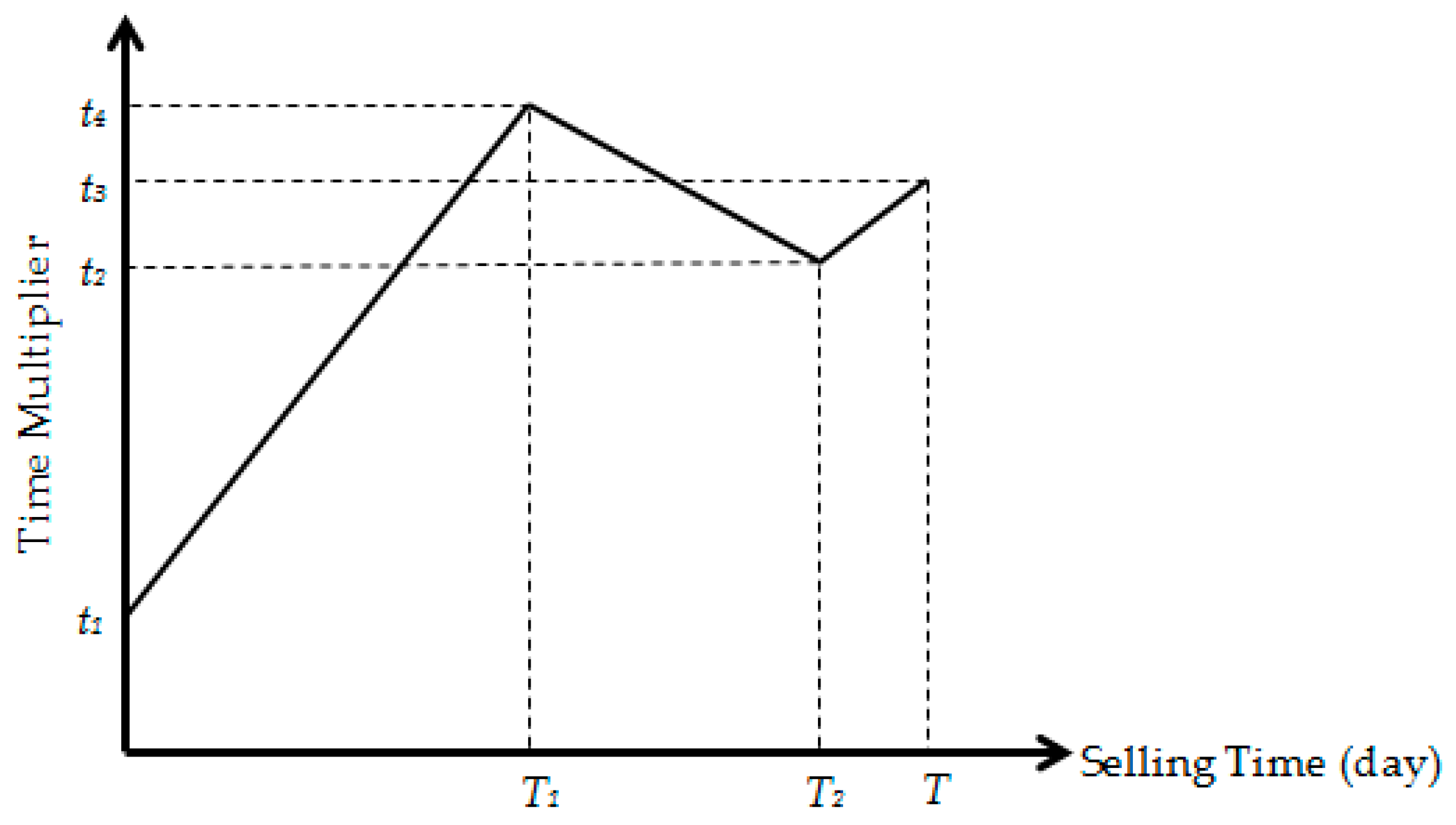
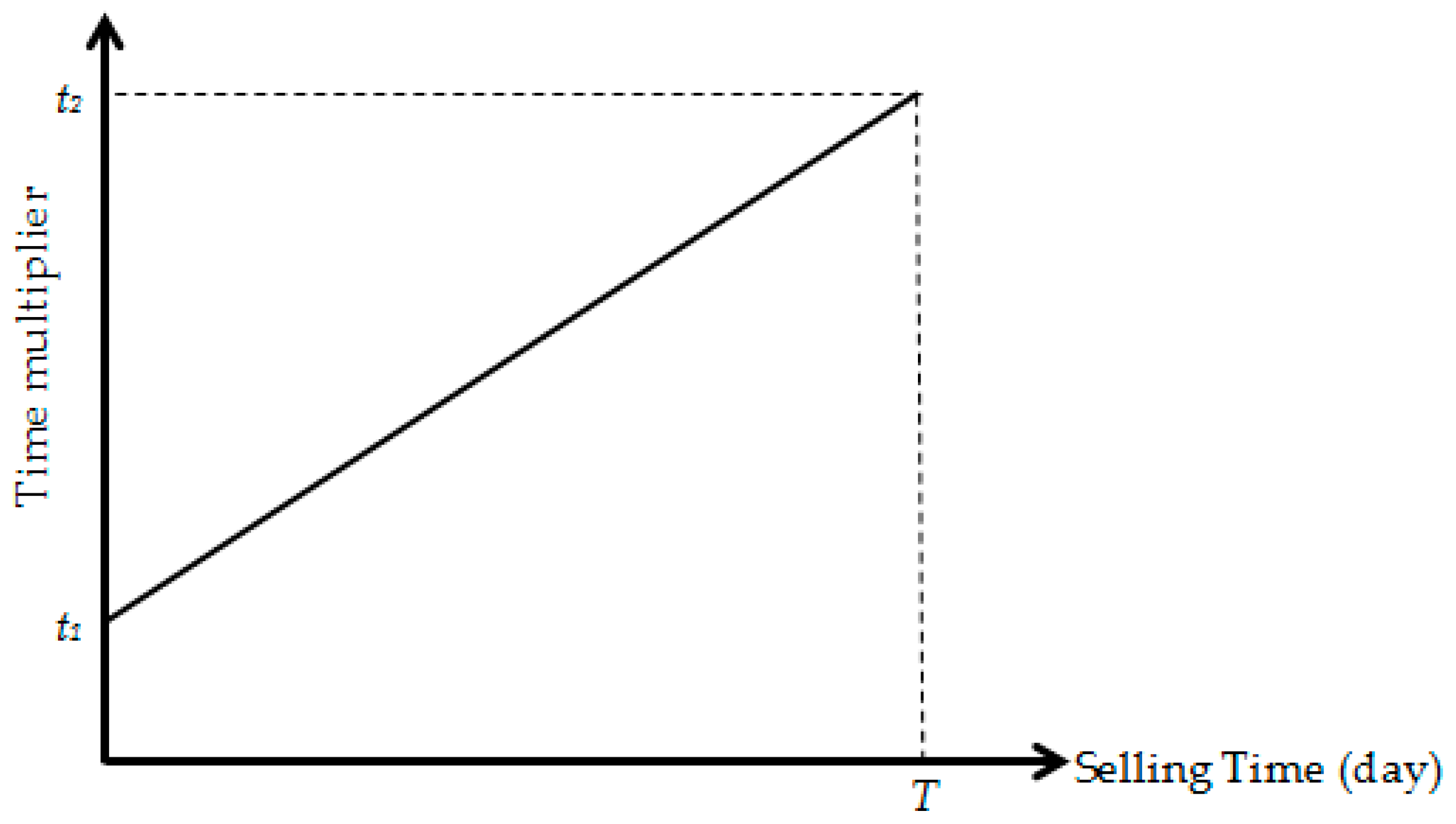
Match tickets are sold in advance. The time from buying the ticket to the starting time of the game is a significant control variable for ticket prices [6]. Two forms of time multiplier are considered, and the behavior of the multipliers is shown in Figure 2 and Figure 3. The x-axis represents the selling time (in days) and the y-axis represents the value of the time multiplier. Change in the time multiplier is assumed to be linear to simplify calculations.
- In the first form, the time multiplier begins at its lowest level (t1) to sell as many tickets as possible by offering the lowest prices initially. As time passes, the time multiplier increases to its highest level (t4) at T1. If there are many tickets available, the time multiplier decreases to (t2) at T2. Towards the end of the selling period, it is assumed that customers are not concerned about the price, so the time multiplier increases to (t3). “T” represents the end of the selling period.
- In the second case, the time multiplier begins at its lowest level (t1) and, as time passes, it increases to (t2). This case is often stated in the sports literature [19,31]. The logic behind this scenario is offering low prices at the beginning to sell as many tickets as possible. Then, the multiplier increases continually towards end of selling period based on the assumption that last-minute spectators are not very concerned about prices.
Inventory Multiplier
The relationship between available tickets and the inventory multiplier is shown in Figure 4. The x-axis represents available tickets, with number as its unit. The number of tickets offered for sale is obtained by subtracting the number of season tickets sold from the total stadium capacity. The y-axis represents the inventory multiplier.
As the inventory decreases, the inventory multiplier increases. Put differently, the inventory multiplier increases based on the assumption that remaining tickets will sell at higher prices. At the beginning, when the number of tickets to be sold is high, the inventory multiplier is at its lowest value (i1). As the number of tickets sold increases, the inventory multiplier rises to its highest value (i2).
2.1.2. Formulation
All multipliers have a significant effect on dynamic ticket prices. As indicated previously, prices should change in a specific interval because of season ticket holders and fans. To ensure this occurs, the chosen average value of every multiplier is 1.25. Otherwise, prices lower than the mean season ticket prices may discourage season ticket holders and excessive prices may alienate fans. There are two cases of the time multiplier. The following equations are obtained for each case. All equations are obtained in a similar way, in which the average value, 1.25, will be equal to the area under the line divided by the range. For instance, for the second case, the third equation is obtained by dividing the area under the line (which is the area of the trapezoid) by the range (which is T) and setting this equal to 1.25.
- t1, t2, t3, T1 and T2 are the optimization variables and t4 is the dependent variable.
- t1 is the optimization variable and t2 is the dependent variable.
- There is only one case for the inventory multiplier, as follows:
To maintain price changes in a certain interval, the constraints in Table 1 were determined. The minimum and maximum limits of T1 and T2 were formed based on the start and end of the selling period, which is 20 days. The minimum and maximum values of inventory multipliers and time multipliers for both cases were determined by trial and error. These limits prevent dynamic prices from being lower than the mean season ticket price and from being high enough to discourage fans.
All constraints attempt to maintain the shape of the multiplier functions. The bounds may be changed based on the problem. The optimization algorithm attempts to find the optimal values of the multipliers within the limits of the constraints. The primary objective of the optimization is to maximize the total revenue. Total revenue generated is calculated as follows:
In this equation, the “t” subscript represents time, “S” represents the length of the selling period, “Pricet” represents the ticket price at time t, and “Demandt” represents the demand for the ticket.
The MATLAB 2015b Simulink tool was used for the optimization. A simulation model was developed for each case of the time multiplier. The optimization tool evaluates different multiplier values until it determines the optimal values. Once the optimum values are obtained, the dynamic prices at any time and inventory level can be obtained.
2.2. Demand Forecasting by a Fuzzy Logic System
Fuzzy logic can be seen as an attempt to mechanize two human capabilities. One is the ability to reason and make rational decisions in the case of uncertain and vague information. The other is the ability to fulfill various physical and mental tasks without requiring any measurements or calculations [32]. The foundation of fuzzy modeling is a rule-based system, also known as a fuzzy inference system (FIS). A fuzzy logic approach provides analysis of the structure of a complex system, in which linguistic terms are used instead of numerical variables to model the system.
There are several steps in designing a fuzzy logic model, as shown in Figure 5. First, the input and output variables are identified. In this study, the input variables are weather, day of game, distance, performance of home team, uncertainty of outcome, and ticket price. These variables were selected based on a comprehensive literature review. As explained in the literature review section, there are various factors that may have an effect on attendance at sports games. In this study, the most common factors were chosen. First, the majority of the studies consider weather or temperature as a significant variable, especially for outdoor events [22,33,34,35,36]. The better the weather, the higher the ticket demand [25]. Second, the geographical distance between the stadiums of the home and away teams is considered to be a significant factor [24,36,37,38]. This factor allows for the effect a local game has on attendance. Third, the day the game is played is also considered to be an effective factor [39,40]. Games on the weekends generally have higher attendance than those on weekdays [25]. Fourth, another input variable is the performance of the home team. Rascher [41] and Bruggink and Eaton [42] believe that the performance of the home team has a larger effect on attendance than that of the away team for Major League Baseball. Forrest and Simmons [38] state that this may be relevant for soccer games in which fans respond to a positive performance by their team. In this study, similar to the study by Forrest and Simmons [38], the performance of the home team is measured as the ratio of points that the team has earned to possible total points to the date of the schedule. Fifth, another factor considered is the uncertainty of outcome. Forrest and Simmons [38] define it as the degree of unpredictability concerning the result of a game. Will [43] found that spectators prefer a more balanced league over a less balanced league. Forrest and Simmons [38] also assert that as uncertainty decreases, the attendance decreases. Therefore, uncertainty of outcome was selected as a determining factor of attendance. The betting odds have been used, as Forrest and Simmons [38] and Peel and Thomas [37] consider them in their studies. They justify the choice of this factor by stating that odds are determined by considering all the other factors affecting game demand, such as injured players, suspended players, and so on. Based on the study by Peel and Thomas [37], Forrest and Simmons [38] conclude that fans prefer potentially close games. Therefore, in this study, the ratio of betting odds is used. The smaller value is divided by the larger value, since evenly matched games attract more spectators. Therefore, the maximum value of uncertainty becomes 1 in the most uncertain case. Finally, ticket price is also considered a significant factor affecting demand [36,44]. High ticket prices might discourage potential spectators [2,3,24]. In addition, the output variable is the ticket demand rate. The stadium capacities of all soccer clubs are different, so as a general term the demand rate is valid for all clubs. Put differently, the demand rate reflects the capacity utilization. To obtain the number of spectators, the demand rate is multiplied by the total number of tickets available for sale.
Second, the fuzzy sets associated with each variable were defined. These sets and the variable labels are shown in Table 2.
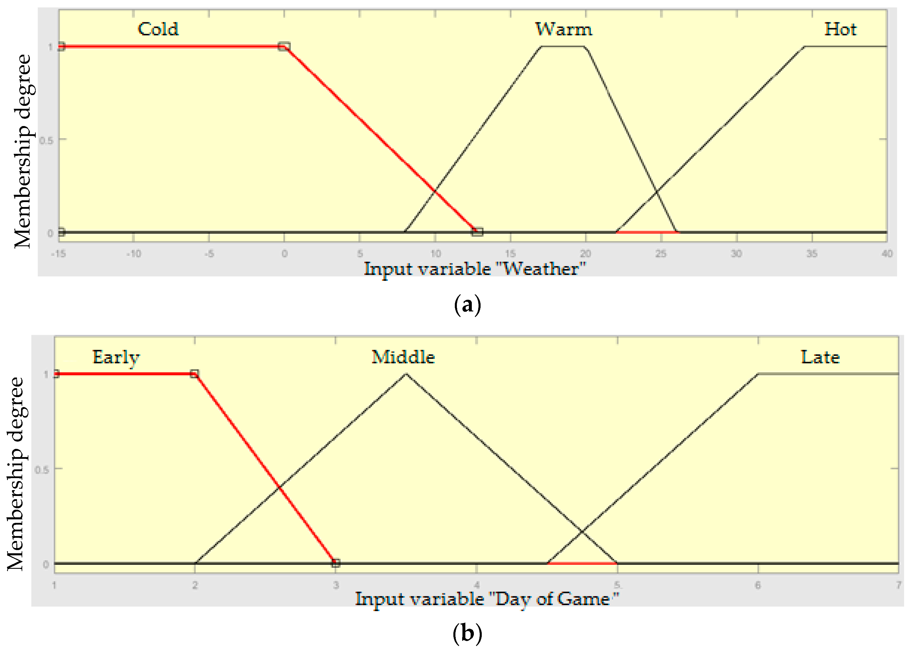
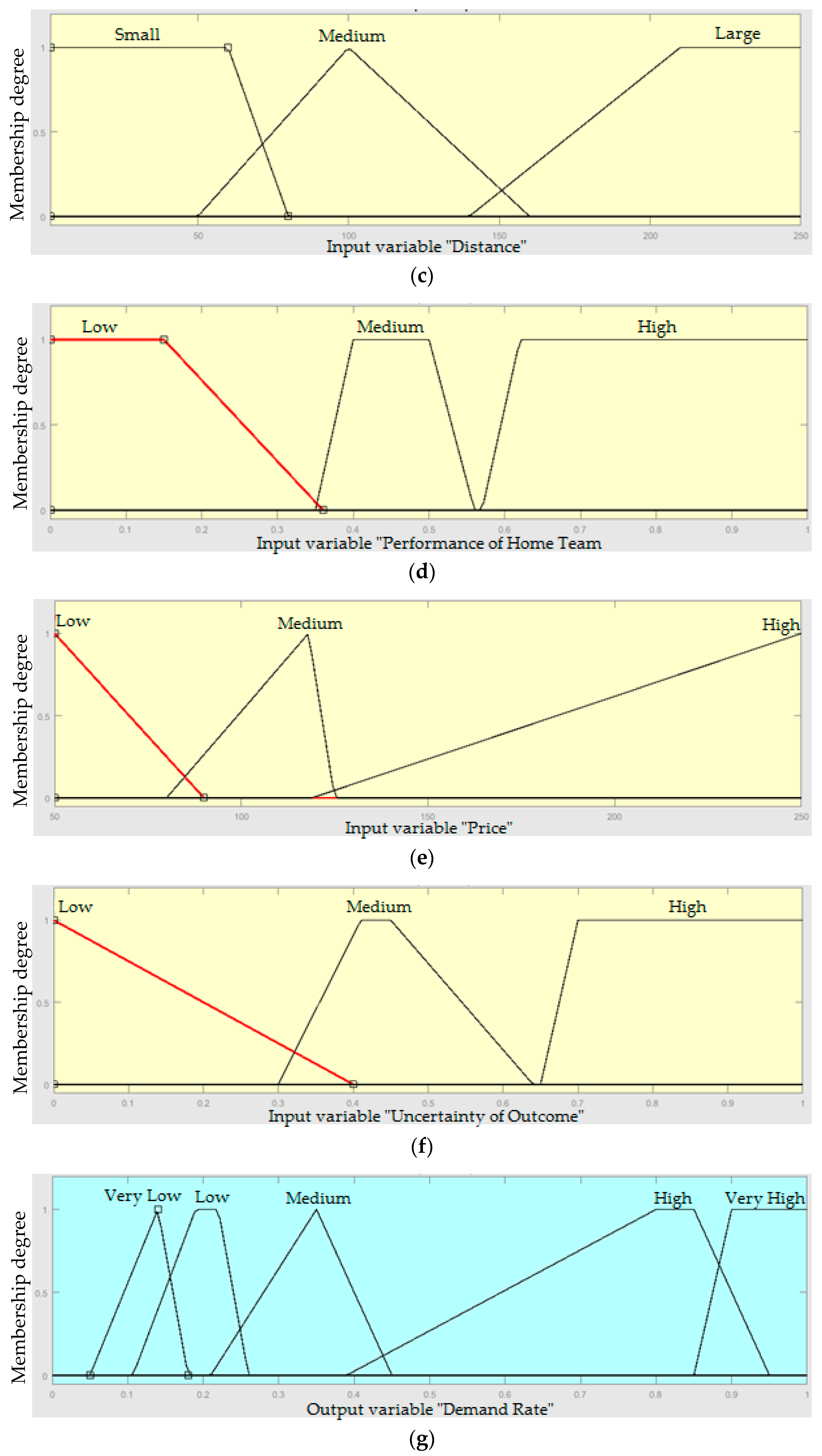
Next, the membership functions were formed for each fuzzy input and output variable. Membership functions illustrate the degree of membership for each value of the variables. The range of values for these functions was determined based on the literature. For example, based on Dobson and Goddard [24], distances of up to 60 m are considered to be small and distances of at least 200 m are considered to be large. Likewise, Butler [35] classifies temperature as cold when it is less than 55 °F and hot if it is greater than 94 °F. The temperature is classified as cold, warm, or hot depending on this range of values. There are different types of membership functions such as triangular, trapezoidal, and sigmoidal. Membership functions should be selected properly since they affect the design of the fuzzy logic controller. In this study, trapezoidal and triangular forms were chosen as the most appropriate after experimenting with the different types. The membership functions that are determined based on input and output variables are shown in Figure 6.
Third, after establishing membership functions, the fuzzy rules (if-then) were generated to establish the relations among the input and output variables. These rules were determined based on expert knowledge and research conducted of sports literature. The basic form of the rule is as follows:
If (condition A) AND If (condition B) Then (consequence).
The calculations are made based on “AND” and “NOT” operators. There were 64 rules formed for this study; an example is as follows:
If (Weather is not Cold) and (DayofGame is Late) and (Distance is Large) and (PerformanceofHomeTeam is High) and (Price is High) and (UncertaintyofOutcome is High) then (DemandRate is High) (1).
As seen in this example, there are six conditions and they are all related to each other with “AND” operators. At the end of each rule, the weight of the rule is shown. In this study, all weights are the same with a value of “1”.
Fourth, the inference process was established. Two of the most commonly used fuzzy inference processes are Mamdani and Sugeno [45]. The consequent of the fuzzy rules determines the primary difference between the two methods. The Mamdani method uses fuzzy sets as the rule consequent whereas the Sugeno method employs linear functions of input variables as the rule consequent. Both methods have advantages. The Mamdani method is intuitive and is well-suited to human input. However, the Sugeno method works well with linear and optimization techniques and is very compatible with mathematical analysis. In this study, the Mamdani-type inference system is used since it relies on expert knowledge, does not require training data, and provides successful results [46,47]. It is also the most commonly seen in the literature. This method has several steps. First, the crisp input variables are fuzzified. In this manner, the degree to which they belong to each of the proper fuzzy sets is determined through membership functions. Second, if a fuzzy rule has more than one antecedent, an “AND” or “OR” fuzzy operator is used to obtain a single number. In the fuzzy logic toolbox, AND methods are min (minimum) and prod (product). The OR methods are max (maximum), and probor (probabilistic OR).
Before applying the third step (the implication method), the rule’s weight is determined. A single number given by the antecedent is the input and a fuzzy set is the output. Implication is implemented for each rule. Fourth, since decisions are made after all rules have been evaluated, the rules must be combined to reach a decision. All outputs are aggregated such that the fuzzy sets that represent each rule’s outputs are combined into a single fuzzy set. Aggregation methods include: max (maximum), probor (probabilistic OR), and sum (simply the sum of each rule’s output set). The final step is defuzzification [48].
The fuzzy results must be defuzzified to obtain crisp numerical values. This occurs by a defuzzification method. The input to the defuzzification process is a fuzzy set and the output is a crisp number. There are several defuzzification methods. The commonly used methods are largest of maximum (LOM), centroid, smallest of maximum (SOM), mean of maximum (MOM), and bisector. In this study, the centroid method, which returns the center of the area under the curve, was chosen because it provides superior results.
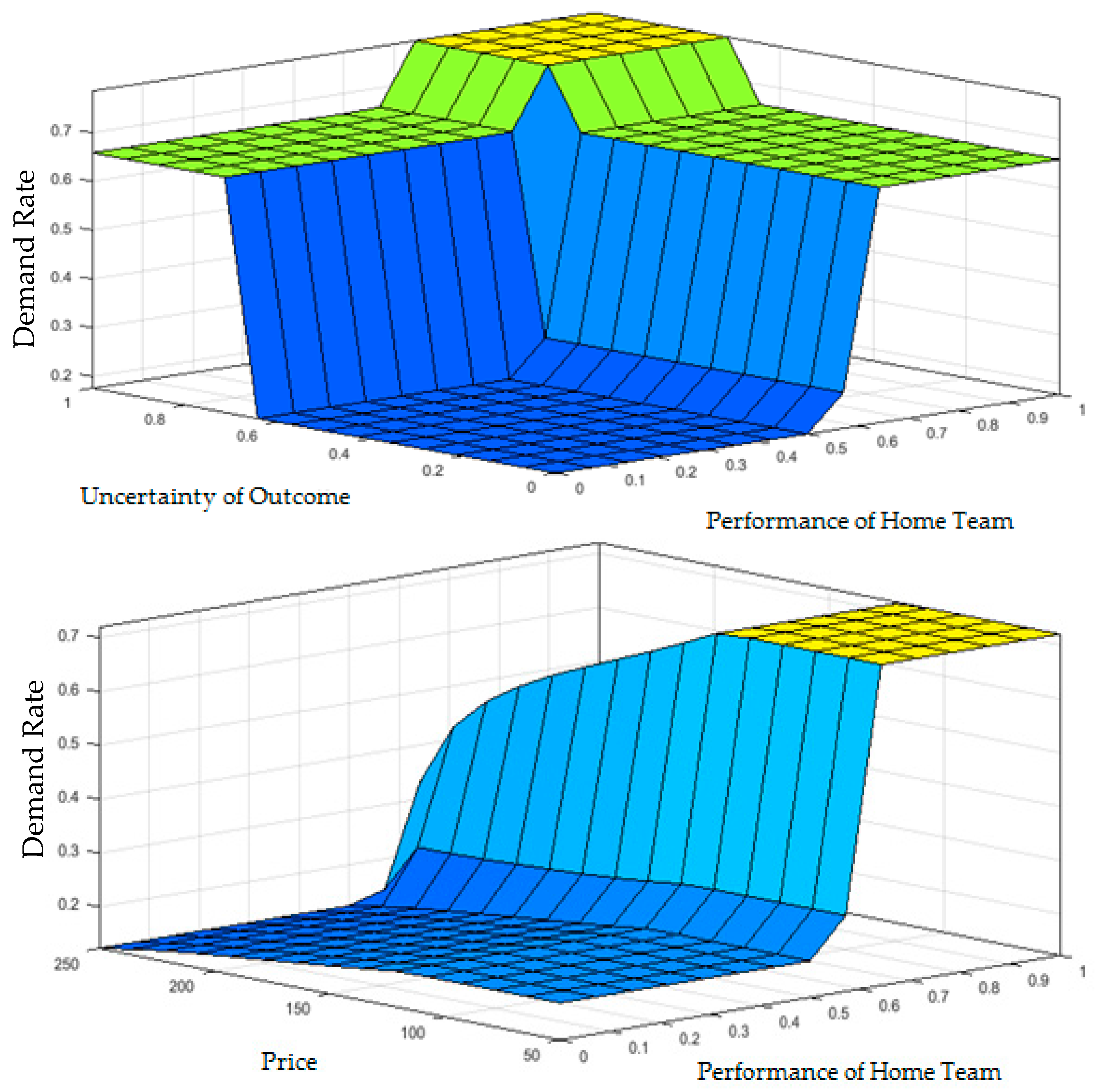
The surface plots of fuzzy rules using different input variables are illustrated in Figure 7.
In this study, the fuzzy logic toolbox of MATLAB 2015b was used to build the fuzzy logic model. By forming and using if-then rules, the demand rate of soccer tickets is estimated based on the weather condition on game day, the day of the game, ground distance between stadiums, performance of the home team, uncertainty of outcome, and price. Only the price might be controlled by the sports club. The remaining variables are exogenous factors that cannot be controlled by the club.
Clearly, soccer tickets are sold before a season starts. Some of the tickets are sold as season tickets for all or some of the season’s games. Therefore, the remaining tickets are sold individually. This study considers the remaining tickets, since their potential purchasers are more sensitive to changes in the performance of the home team and the prestige of the visiting team. They are also likely to be more selective in their choice of games [24].
2.3. Application
This section contains two scenarios. First, to evaluate the results of the proposed fuzzy logic approach, the attendance data of AC Milan, an Italian football club, was considered. The attendance at some games played during the past three seasons was analyzed and compared with the forecasted demand rates. Second, to test the effectiveness of the proposed dynamic pricing models, the models were applied to a subset of the tickets for a specific game. The game was played on a Saturday with an average temperature of 10 °C. The number of tickets to be sold at a price of €118 was 1800. The mean season ticket price was €90. It is assumed that 100 customers accessed the system daily and that the game tickets were offered for sale 20 days in advance. The ground distance between the stadiums of the teams was 85 m. Based on the number of points earned by the home team, the performance of the home team was calculated as 0.67. Based on the betting odds obtained, the uncertainty of the outcome was calculated as 0.40.
To find optimal parameters of the multipliers, as mentioned previously, a simulation model was designed in MATLAB 2015b Simulink. The proposed simulation model is shown in Figure 8.
As seen in Figure 8, demand at different price levels is forecasted. Based on tickets sold and the time, the time and inventory multipliers are calculated. These are used to determine the dynamic prices. After determining the prices, the revenue is calculated. These processes are repeated until the selling period is over. The optimization algorithm attempts to find the optimal parameters of the multipliers that produce the maximum revenue. Once the optimal parameters are obtained, the optimal dynamic prices can be calculated.
3. Results and Discussion
The results are provided in two sections: the results of demand forecasting and the results of the dynamic pricing model.
3.1. Results of Demand Forecasting
As explained in the previous sections, the input variables are weather, day of game, distance, performance of home team, price, and uncertainty of outcome. All data was obtained from different sources. First, the average temperature (°C) on the game day was obtained from the website https://www.wunderground.com. Second, geographical ground distances were collected from the website https://www.distancecalculator.net. Third, to evaluate the performance of the home team, the number of points earned by the team was obtained. The ticket prices were collected from the club’s website. Lastly, the uncertainty of outcome was calculated based on data collected from the website http://www.football-data.co.uk. The output of the demand forecasting is the demand rate of games based on these variables.
At the modeling stage, the season tickets were excluded, but the match day tickets were considered. The days were numbered from Monday to Sunday, where 1 represents Monday, 2 represents Tuesday, and so on. The ground distances between stadiums that are greater than 250 m were accepted as 250 m (large distances). The data that was collected and calculated is given in Table 3.
To compare the results of the fuzzy logic model with real data, the mean absolute percentage error (MAPE) and mean squared error (MSE) were calculated. The calculated MSE is 0 and the MAPE is 0.1. Based on these results, it can be concluded that the results of the proposed fuzzy logic approach are successful and highly competitive.
3.2. Results of Dynamic Ticket Pricing
As explained in the previous sections, there are two cases of the proposed model. To evaluate the success of the models, the revenue generated from each was compared with the static pricing, in which the price does not change at any point in the selling period. After the simulation was executed one thousand times, the optimum values of the multipliers were obtained as t1 = 0.9002, t2 = 1.2, t3 = 1.3896, i1 = 1.156, T1 = 2.6189, T2 = 9.006 and t1 = 1.0037, i1 = 1.25 for Cases I and II, respectively. After obtaining these values, the dynamic prices at any selling period and at any inventory level can be calculated. Based on the optimization results, the revenue for the two cases and static pricing are provided in Table 4.
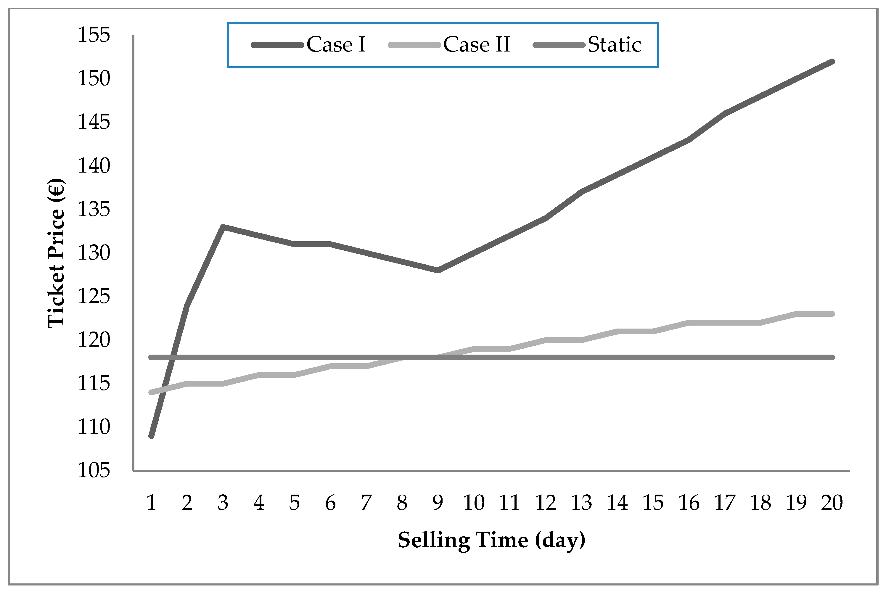
As seen in Table 4, both dynamic pricing models generated more revenue than the static pricing strategy. There were 1800 tickets available. Quantities of 630, 660, and 660 tickets were sold for Case I, Case II, and the static pricing strategy, respectively. Case I is proposed in this study, while Case II is stated commonly in the sports literature. The static pricing strategy is adopted by almost all soccer clubs. According to the comparison results, the highest revenue is obtained from Case I while the lowest revenue is obtained from the static pricing strategy. The ticket prices at different points in the selling period are shown in Figure 9.
The results show that prices fluctuate in Cases I and II. However, ticket prices remain the same during the selling period with a static pricing strategy. The demand levels are different at each price level.
4. Conclusions
A dynamic ticket pricing model for soccer clubs is proposed in this study. Dynamic ticket prices are determined based on time and inventory multipliers. Two cases of the time multiplier were chosen to allow comparisons among revenues. The essential function of the model is to determine the optimal parameters of the multipliers with the goal of maximizing revenue. Once the parameters are obtained, dynamic prices at any time point and at any inventory level can be calculated easily. The model requires demand rates at different price levels, and the required demand rates are forecasted by the proposed fuzzy logic system.
One of the primary contributions of this study is forecasting the demand with a unique fuzzy logic approach. Fuzzy if-then rules were generated for this purpose. Fuzzy logic is proven to be successful at forecasting. This study demonstrates that it provides competitive forecasting results for soccer games. The results were compared with real data and were found to be effective. In summary, it can be an alternative to classic regression models for forecasting attendance at sports games. Another contribution of this paper is the development of a mathematical model of dynamic pricing for soccer games. Almost all the dynamic pricing studies in sports attempt to explain the effective factors for dynamic pricing models and/or attempt to address dynamic pricing models from a managerial perspective. Therefore, it is significant to introduce a new mathematical model. Two cases were considered, and their results were compared with the results of the static pricing strategy. The results show that the model assists in generating an increase of up to 8.95% in ticket sales revenue. Considering one hundred million dollars of match day revenue, even a 0.01% increase has substantial value. With a few modifications, the model can be implemented for other sports disciplines.
An additional multiplier that reflects the characteristics of the game to ticket prices could be included in the model. For instance, a calculated uncertainty of outcome might be used for that purpose. It does not change the structure of the model but merely adds an additional multiplier to calculate the uncertainty of the game’s outcome.
Both of the proposed models may have some limitations. Adding consideration of strategic customers might enhance the applicability of the dynamic pricing model. Additionally, considering consumer resale effects might also improve the quality of the model. Finally, the input variables that are used to forecast the demand rate may be revised and improved if required. The fuzzy sets may be enhanced as well. There may be some other effective determinants of the demand to consider.
Author Contributions
Mehmet Şahin collected the data, Mehmet Şahin and Rızvan Erol designed the models; Mehmet Şahin and Rızvan Erol analyzed the results; Mehmet Şahin wrote the paper.
Conflicts of Interest
The authors declare no conflict of interest.
References
- Boor, S.; Bosshardt, A.; Green, M.; Hanson, C.; Savage, J.; Shaffer, A.; Winn, C. Top of the Table—Football Money League; Jones, D., Ed.; Deloitte: New York, NY, USA, 2016. [Google Scholar]
- Drayer, J.; Shapiro, S.L.; Lee, S. Dynamic ticket pricing in sport: An agenda for research and practice. Sports Mark. Q. 2012, 21, 184–194. [Google Scholar]
- Nufer, G.; Fischer, J. Ticket pricing in European football—Analysis and implications. Int. J. Hum. Mov. Sports Sci. 2013, 1, 49–60. [Google Scholar]
- Rascher, D.A.; McEvoy, C.D.; Nagel, M.S.; Brown, M.T. Variable ticket pricing in major league baseball. J. Sport Manag. 2007, 21, 407–437. [Google Scholar] [CrossRef]
- Parris, D.L.; Drayer, J.; Shapiro, S.L. Developing a pricing strategy for the Los Angeles Dodgers. Sports Mark. Q. 2012, 21, 256–264. [Google Scholar]
- Shapiro, S.L.; Drayer, J. A new age of demand-based pricing: An examination of dynamic ticket pricing and secondary market prices in Major League Baseball. J. Sport Manag. 2012, 26, 532–546. [Google Scholar] [CrossRef]
- Van Ryzin, G.J.; Talluri, K.T. Emerging Theory, Methods, and Applications. In An Introduction to Revenue Management; INFORMS: Catonsville, MD, USA, 2005; pp. 142–194. [Google Scholar]
- Bitran, G.R.; Mondschein, S.V. An application of yield management to the hotel industry considering multiple day stays. Oper. Res. 1995, 43, 427–443. [Google Scholar] [CrossRef]
- Otero, D.F.; Akhavan-Tabatabaei, R. A stochastic dynamic pricing model for the multiclass problems in the airline industry. Eur. J. Oper. Res. 2015, 242, 188–200. [Google Scholar] [CrossRef]
- Zhang, D.; Weatherford, L. Dynamic pricing for network revenue management: A new approach and application in the hotel industry. INFORMS J. Comput. 2016, 29, 18–35. [Google Scholar] [CrossRef]
- Kimes, S.E. Yield management: A tool for capacity-considered service firms. J. Oper. Manag. 1989, 8, 348–363. [Google Scholar] [CrossRef]
- Kimes, S.E.; Chase, R.B.; Choi, S.; Lee, P.Y.; Ngonzi, E.N. Restaurant revenue management. Cornell Hotel Restaur. Adm. Q. 1998, 39, 32–39. [Google Scholar] [CrossRef]
- Phumchusri, N.; Swann, J.L. Scaling the house: Optimal seating zones for entertainment venues when location of seats affects demand. Int. J. Rev. Manag. 2014, 8, 56–98. [Google Scholar] [CrossRef]
- Davenport, T.H. Analytics in Sports: The New Science of Winning; International Institute for Analytics: Portlang, OR, USA, 2014. [Google Scholar]
- PwC. At the Gate and Beyond—Outlook for the Sports Market in North America through 2019. In PwC Sports Outlook; Jones, A.W., Ed.; PwC: London, UK, 2015. [Google Scholar]
- Kemper, C.; Breuer, C. How efficient is dynamic pricing for sport events? Designing a dynamic pricing model for Bayern Munich. Int. J. Sport Financ. 2016, 11, 4. [Google Scholar]
- Marburger, D.R. Optimal ticket pricing for performance goods. Manag. Decis. Econ. 1997, 18, 375–381. [Google Scholar] [CrossRef]
- Kemper, C.; Breuer, C. What factors determine the fans’ willingness to pay for Bundesliga tickets? An analysis of ticket sales in the secondary market using data from ebay.de. Sport Mark. Q. 2015, 24, 142. [Google Scholar]
- Kemper, C.; Breuer, C. Dynamic ticket pricing and the impact of time—An analysis of price paths of the English soccer club Derby County. Eur. Sport Manag. Q. 2016, 16, 233–253. [Google Scholar] [CrossRef]
- Hart, R.; Hutton, J.; Sharot, T. A statistical analysis of association football attendances. Appl. Stat. 1975, 24, 17–27. [Google Scholar] [CrossRef]
- Pawlowski, T.; Anders, C. Stadium attendance in German professional football—The (un)importance of uncertainty of outcome reconsidered. Appl. Econ. Lett. 2012, 19, 1553–1556. [Google Scholar] [CrossRef]
- Martins, A.M.; Cró, S. The Demand for Football in Portugal: New Insights on Outcome Uncertainty. J. Sports Econ. 2016. [Google Scholar] [CrossRef]
- Reilly, B. The demand for league of Ireland football. Econ. Soc. Rev. 2015, 46, 485–509. [Google Scholar]
- Dobson, S.; Goddard, J. The Economics of Football; Cambridge University Press: Cambridge, UK, 2011. [Google Scholar]
- García, J.; Rodríguez, P. The determinants of football match attendance revisited: Empirical evidence from the Spanish football league. J. Sports Econ. 2002, 3, 18–38. [Google Scholar] [CrossRef]
- Baranzini, A.; Ramirez, J.V.; Weber, S. The demand for football in Switzerland: An empirical estimation. SSRN Electron. J. 2008. [Google Scholar] [CrossRef]
- DeSchriver, T.D.; Rascher, D.A.; Shapiro, S.L. If we build it, will they come? Examining the effect of expansion teams and soccer-specific stadiums on Major League Soccer attendance. Sport Bus. Manag. Int. J. 2016, 6, 205–227. [Google Scholar] [CrossRef]
- Bayoumi, A.E.-M.; Saleh, M.; Atiya, A.F.; Aziz, H.A. Dynamic pricing for hotel revenue management using price multipliers. J. Rev. Pricing Manag. 2013, 12, 271–285. [Google Scholar] [CrossRef]
- Dorgham, K.; Saleh, M.; Atiya, A.F. A Novel Dynamic Pricing Model for the Telecommunications Industry. In Modelling, Computation and Optimization in Information Systems and Management Sciences; Springer: Berlin, Germany, 2015; pp. 129–140. [Google Scholar]
- Coşgun, Ö.; Ekinci, Y.; Yanık, S. Fuzzy rule-based demand forecasting for dynamic pricing of a maritime company. Knowl. Based Syst. 2014, 70, 88–96. [Google Scholar] [CrossRef]
- Shapiro, S.L.; Drayer, J. An examination of dynamic ticket pricing and secondary market price determinants in Major League Baseball. Sport Manag. Rev. 2014, 17, 145–159. [Google Scholar] [CrossRef]
- Zadeh, L.A. A new direction in AI: Toward a computational theory of perceptions. AI Mag. 2001, 22, 73. [Google Scholar]
- Drever, P.; McDonald, J. Attendances at South Australian football games. Int. Rev. Sport Sociol. 1981, 16, 103–113. [Google Scholar] [CrossRef]
- Welki, A.M.; Zlatoper, T.J. US professional football game-day attendance. Atl. Econ. J. 1999, 27, 285–298. [Google Scholar] [CrossRef]
- Butler, M.R. Interleague play and baseball attendance. J. Sports Econ. 2002, 3, 320–334. [Google Scholar] [CrossRef]
- Borland, J.; MacDonald, R. Demand for sport. Oxf. Rev. Econ. Policy 2003, 19, 478–502. [Google Scholar] [CrossRef]
- Peel, D.A.; Thomas, D.A. The demand for football: Some evidence on outcome uncertainty. Empir. Econ. 1992, 17, 323–331. [Google Scholar] [CrossRef]
- Forrest, D.; Simmons, R. Outcome uncertainty and attendance demand in sport: The case of English soccer. J. R. Stat. Soc. Ser. D 2002, 51, 229–241. [Google Scholar] [CrossRef]
- Buraimo, B.; Simmons, R. Do sports fans really value uncertainty of outcome? Evidence from the English Premier League. Int. J. Sport Financ. 2008, 3, 146. [Google Scholar]
- Cox, A. Spectator demand, uncertainty of results, and public interest: Evidence from the English Premier League. J. Sports Econ. 2015. [Google Scholar] [CrossRef] [Green Version]
- Rascher, D.A. A test of the optimal positive production network externality in Major League Baseball. Sports, Economics: Current Research, 1999. Available online: https://ssrn.com/abstract=81914 (accessed on 1 October 2017).
- Bruggink, T.H.; Eaton, J.W. Rebuilding attendance in Major League Baseball: The demand for individual games. In Baseball Economics: Current Research; Praeger: Westport, NY, USA, 1996; pp. 9–31. [Google Scholar]
- Will, D.H. The Federation’s viewpoint on the new transfer rules. In Competition Policy and Professional Sports: Europe after the Bosman Case; ELS Belgium: Brussels, Belgium, 1999. [Google Scholar]
- Boyd, D.W.; Boyd, L.A. The home field advantage: Implications for the pricing of tickets to professional team sporting events. J. Econ. Financ. 1998, 22, 169–179. [Google Scholar] [CrossRef]
- Zimmermann, H.-J. Fuzzy Set Theory—And Its Applications; Springer Science & Business Media: Berlin, Germany, 2011. [Google Scholar]
- Mamdani, E.H. Application of fuzzy algorithms for control of simple dynamic plant. Proc. Inst. Electr. Eng. 1974, 121, 1585–1588. [Google Scholar] [CrossRef]
- Sugeno, M. Industrial Applications of Fuzzy Control; Elsevier Science Inc.: Amsterdam, The Netherlands, 1985. [Google Scholar]
- Negnevitsky, M. Artificial Intelligence: A Guide to Intelligent Systems; Pearson Education: London, UK, 2005. [Google Scholar]
Figure 1.
Framework of the proposed model.
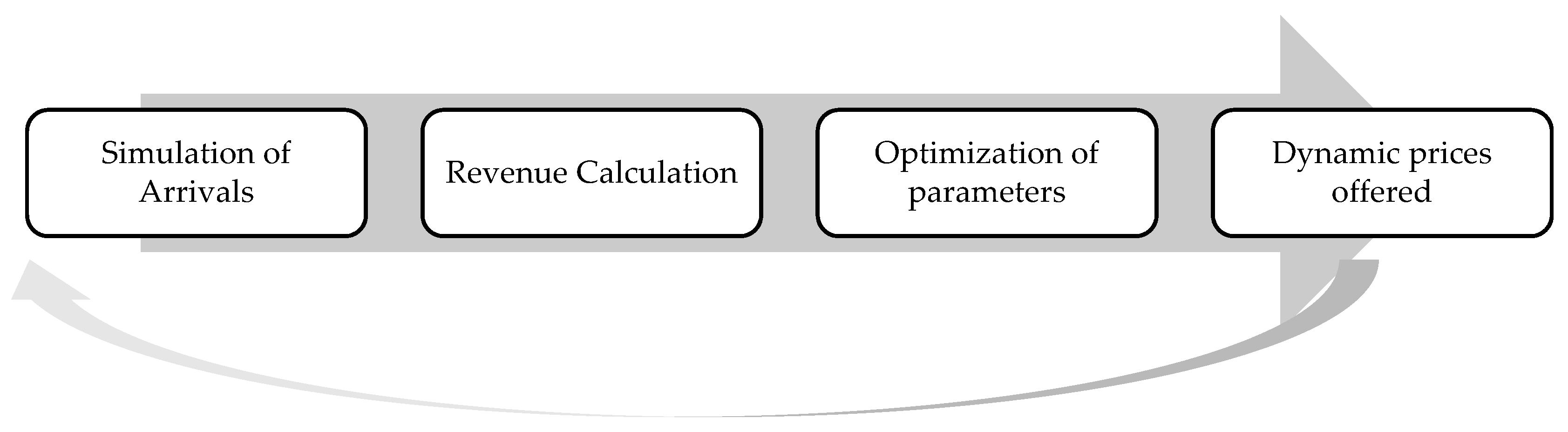
Figure 2.
Time multiplier—Case I.

Figure 3.
Time multiplier—Case II.

Figure 4.
Inventory multiplier.
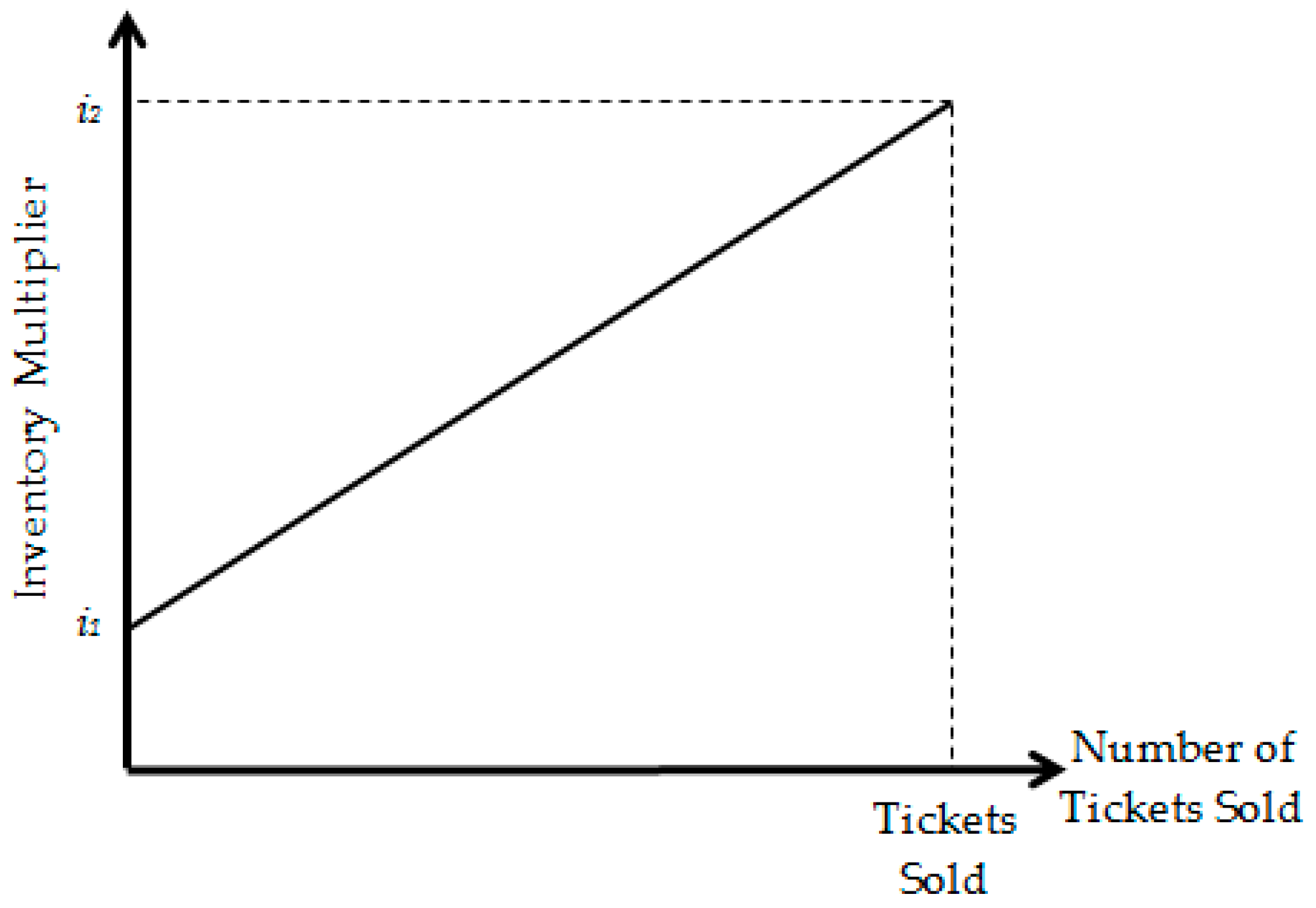
Figure 5.
Steps of the proposed fuzzy logic approach.

Figure 6.
Membership functions of the input variables: (a) weather, (b) day of game, (c) distance, (d) performance of home team, (e) price, (f) uncertainty of outcome, and the output variable: (g) demand rate.
Figure 6.
Membership functions of the input variables: (a) weather, (b) day of game, (c) distance, (d) performance of home team, (e) price, (f) uncertainty of outcome, and the output variable: (g) demand rate.


Figure 7.
Surface plots of fuzzy rules using different input variables.

Figure 8.
Proposed simulation model.
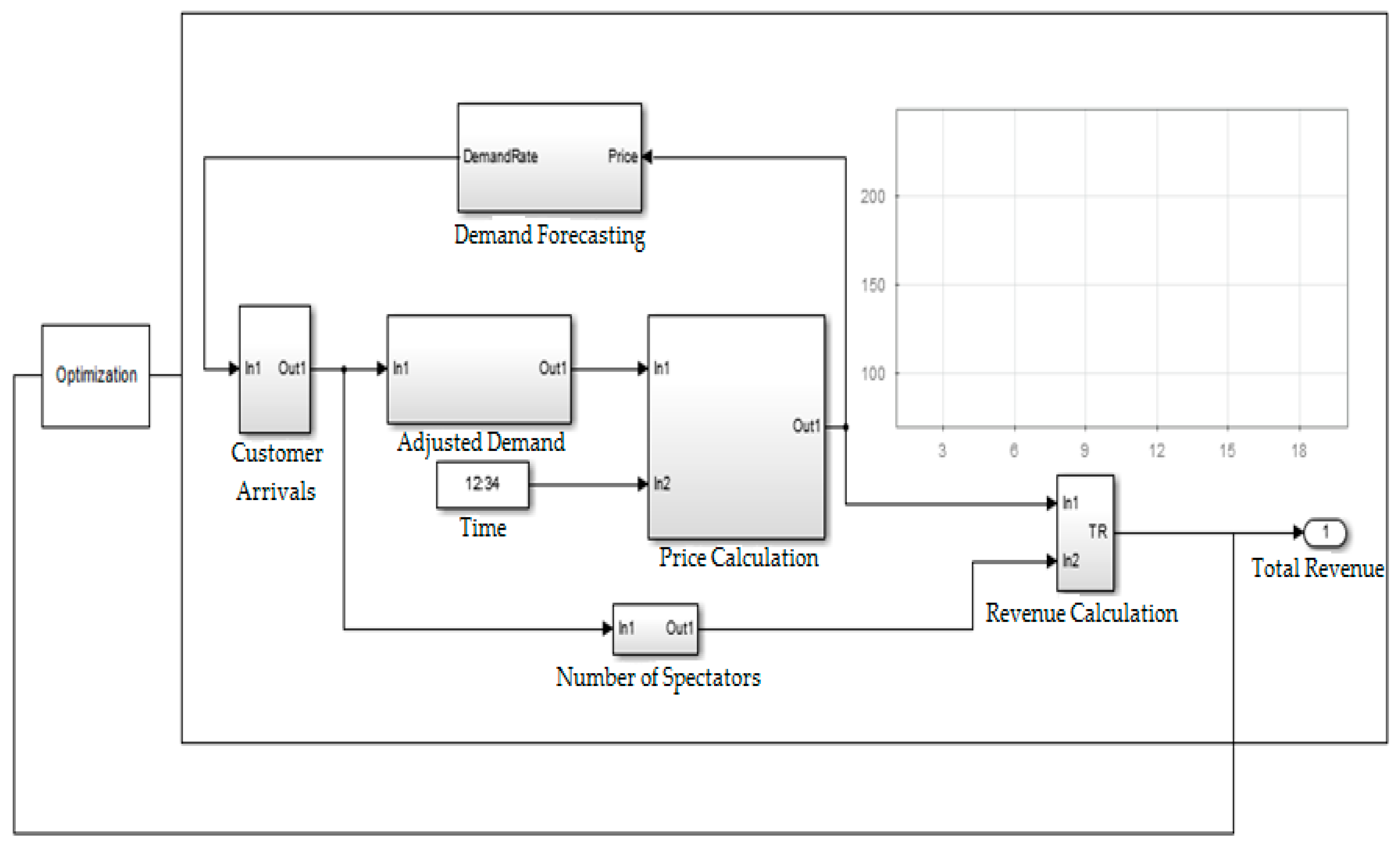
Figure 9.
Dynamic ticket prices for Case I, Case II, and static pricing strategy.

Table 1.
Constraints of the model.
| Inventory Multipliers | Time Multiplier (Case I) | Time Multiplier (Case II) |
|---|---|---|
Table 2.
Fuzzy sets of input and output variables.
| Fuzzy Sets of Input Variables | Fuzzy Sets of Output Variable | |||||
|---|---|---|---|---|---|---|
| Weather (°C) | Day of Game | Distance (m) | Performance of Home Team | Price | Uncertainty of Outcome | Demand Rate |
| Cold | Early | Small | Low | Low | Low | Very Low |
| Warm | Middle | Medium | Medium | Medium | Medium | Low |
| Hot | Late | Large | High | High | High | Medium |
| - | - | - | - | - | - | High |
| - | - | - | - | - | - | Very High |
Table 3.
Data of soccer games and demand rates.
| Game No. | Temperature (°C) | Day of Game | Distance (m) | Performance of Home Team | Price | Uncertainty of Outcome | Demand Rate (Actual) | Demand Rate (Fuzzy Logic) |
|---|---|---|---|---|---|---|---|---|
| 1 | 24 | 7 | 241 | 0.50 | 118 | 0.33 | 0.186 | 0.192 |
| 2 | 19 | 2 | 364 | 0.50 | 118 | 0.63 | 0.158 | 0.123 |
| 3 | 10 | 6 | 85 | 0.67 | 118 | 0.40 | 0.934 | 0.937 |
| 4 | 12 | 7 | 376 | 0.63 | 118 | 0.18 | 0.316 | 0.337 |
| 5 | 8 | 7 | 0 | 0.69 | 118 | 0.93 | 0.966 | 0.935 |
| 6 | 6 | 7 | 739 | 0.69 | 118 | 0.13 | 0.338 | 0.335 |
| 7 | 2 | 6 | 37 | 0.67 | 118 | 0.50 | 0.301 | 0.336 |
| 8 | 4 | 7 | 205 | 0.57 | 118 | 0.61 | 0.256 | 0.214 |
| 9 | 11 | 6 | 95 | 0.60 | 118 | 0.34 | 0.289 | 0.313 |
| 10 | 14 | 7 | 925 | 0.60 | 118 | 0.10 | 0.320 | 0.287 |
| 11 | 16 | 7 | 140 | 0.56 | 118 | 0.16 | 0.387 | 0.337 |
| 12 | 27 | 6 | 206 | 0.00 | 118 | 0.21 | 0.245 | 0.209 |
| 13 | 20 | 6 | 925 | 0.33 | 118 | 0.35 | 0.234 | 0.192 |
| 14 | 12 | 7 | 103 | 0.42 | 118 | 0.35 | 0.298 | 0.327 |
| 15 | 2 | 6 | 95 | 0.51 | 118 | 0.26 | 0.212 | 0.231 |
| 16 | 6 | 3 | 140 | 0.55 | 118 | 0.21 | 0.196 | 0.189 |
| 17 | 8 | 7 | 0 | 0.52 | 118 | 0.72 | 0.951 | 0.935 |
| 18 | 6 | 7 | 241 | 0.57 | 118 | 0.22 | 0.134 | 0.189 |
| 19 | 5 | 6 | 98 | 0.56 | 118 | 0.35 | 0.235 | 0.265 |
| 20 | 11 | 7 | 364 | 0.55 | 118 | 0.50 | 0.231 | 0.191 |
| 21 | 16 | 6 | 85 | 0.53 | 118 | 0.51 | 0.924 | 0.939 |
| 22 | 17 | 4 | 118 | 0.53 | 118 | 0.19 | 0.153 | 0.192 |
| 23 | 20 | 7 | 85 | 1 | 118 | 0.70 | 0.978 | 0.939 |
| 24 | 11 | 7 | 205 | 0.67 | 118 | 0.57 | 0.311 | 0.336 |
| 25 | 7 | 7 | 0 | 0.52 | 118 | 0.97 | 0.986 | 0.934 |
| 26 | 11 | 7 | 560 | 0.43 | 118 | 0.42 | 0.184 | 0.191 |
Table 4.
Revenue obtained for Case I, Case II, and static pricing strategy.
| Pricing Strategy | Revenue (€) | Difference (%) | |
|---|---|---|---|
| Dynamic Pricing | Case I | 84,849 | 8.95 |
| Case II | 78,474 | 0.76 | |
| Static Pricing | - | 77,880 | - |
© 2017 by the authors. Licensee MDPI, Basel, Switzerland. This article is an open access article distributed under the terms and conditions of the Creative Commons Attribution (CC BY) license (http://creativecommons.org/licenses/by/4.0/).
Share and Cite
MDPI and ACS Style
Şahin, M.; Erol, R. A Dynamic Ticket Pricing Approach for Soccer Games. Axioms 2017, 6, 31. https://doi.org/10.3390/axioms6040031
AMA Style
Şahin M, Erol R. A Dynamic Ticket Pricing Approach for Soccer Games. Axioms. 2017; 6(4):31. https://doi.org/10.3390/axioms6040031
Chicago/Turabian StyleŞahin, Mehmet, and Rızvan Erol. 2017. "A Dynamic Ticket Pricing Approach for Soccer Games" Axioms 6, no. 4: 31. https://doi.org/10.3390/axioms6040031
Note that from the first issue of 2016, this journal uses article numbers instead of page numbers. See further details here.