Article

Limiting Approach to Generalized Gamma Bessel Model via Fractional Calculus and Its Applications in Various Disciplines

Indian Statistical Institute(ISI), Chennai CIT Campus, Taramani, Chennai 600113, India
Axioms 2015, 4(3), 385-399; https://doi.org/10.3390/axioms4030385
Submission received: 15 July 2015 / Revised: 10 August 2015 / Accepted: 10 August 2015 / Published: 26 August 2015

Abstract

:
The essentials of fractional calculus according to different approaches that can be useful for our applications in the theory of probability and stochastic processes are established. In addition to this, from this fractional integral, one can list out almost all of the extended densities for the pathway parameter q < 1 and q 1 . Here, we bring out the idea of thicker- or thinner-tailed models associated with a gamma-type distribution as a limiting case of the pathway operator. Applications of this extended gamma model in statistical mechanics, input-output models, solar spectral irradiance modeling, etc., are established.
MSC classification:
MSC (2000) 26A33, 33C10, 33B15

1. Introduction

In recent years, considerable interest has been shown in so-called fractional calculus, which allows one to consider integration and differentiation of any order, not necessarily integer. Fractional calculus is a rapidly growing field both in theory and in applications to real-world problems. There is a revived interest in fractional integrals and fractional derivatives due to their recently-found applications in reaction, diffusion, reaction-diffusion problems, in solving certain partial differential equations, in input-output models and related areas; see, for example [1,2,3,4,5,6]. There are many books in the area, some of which are [7,8,9,10,11]. The classical left- and right-hand-sided Riemann–Liouville fractional integral operators of order α C , ( α ) > 0 , are defined as:
0 D x α f = ( I 0 + α f ) ( x ) = 1 Γ ( α ) o x ( x t ) α 1 f ( t ) d t , x > 0 , ( α ) > 0
x D α f = ( I α f ) ( x ) = 1 Γ ( α ) x ( t x ) α 1 f ( t ) d t , x > 0 , ( α ) > 0
The traditional special functions are also related to the classical fractional calculus (FC) and later to the generalized fractional calculus and are shown to be representable as fractional order integration or differentiation operators of some basic elementary functions. Such relations provided some alternative definitions for the special functions by means of Poisson-type and Euler-type integral representations and Rodrigues-type differential formulas. An example of such a unified approach on special functions, based on a generalized fractional calculus, can be seen in [8]. The essentials of fractional calculus according to different approaches that can be useful for our applications in the theory of probability and stochastic processes are established with the help of the pathway idea in [12].
The pathway idea was originally proposed by Mathai in the 1970s in connection with population models and later rephrased and extended in [12] to cover scalar, as well as matrix cases, and it was made suitable for modeling data from statistical and physical situations. The main idea behind the derivation of this model is the switching properties of going from one family of functions to another and, yet, another family of functions. It is shown that through a parameter q, called the pathway parameter, one can connect a generalized Type 1 beta family of densities, a generalized Type 2 beta family of densities and generalized gamma family of densities, in the scalar, as well as in the matrix cases, also in the real and complex domains. It is shown that when the model is applied to physical situations, then the current hot topics of Tsallis statistics and superstatistics in statistical mechanics become special cases of the pathway model, and the model is capable of capturing many stable situations, as well as the unstable or chaotic neighborhoods of the stable situations and transitional stages. Mathai [12] deals mainly with rectangular matrix-variate distributions, and the scalar case is a particular case there. For the real scalar case, the pathway model is the following:
h 1 ( x ) = k 1 x γ 1 [ 1 a ( 1 q ) x θ ] η 1 q , 1 a ( 1 q ) x θ > 0 , a , θ , γ , η > 0 , q < 1
where k 1 is the normalizing constant if a statistical density is needed. For q < 1 , the model remains as a generalized Type 1 beta model in the real case. Other cases available are the regular Type 1 beta density, Pareto density, power function, triangular and related models. Observe that Equation (3) is a model with the right tail cut off. When q > 1 , we may write 1 q = ( q 1 ) , q > 1 , so that h 2 ( x ) assumes the form:
h 2 ( x ) = k 2 x γ 1 [ 1 + a ( q 1 ) x θ ] η q 1 , x 0 , a , θ , γ , η > 0 , q > 1
which is a generalized Type 2 beta model for real x, and k 2 is the normalizing constant, if a statistical density is required. Beck and Cohen’s superstatistics belongs to this case Equation (4), and dozens of published papers are available on the topic of superstatistics in astrophysics. For γ = 1 , a = 1 , θ = 1 , we have Tsallis statistics for q > 1 from Equation (4). Other standard distributions coming from this model are the regular Type 2 beta, the F-distribution, L e ´ vi models and related models. When q 1 , the forms in Equations (3) and (4) reduce to:
h 3 ( x ) = k 3 x γ 1 e b x θ , x 0 , b = a η > 0 , γ , θ > 0
where k 3 is the normalizing constant. This includes generalized gamma, gamma, exponential, chi-square, Weibull, Maxwell–Boltzmann, Rayleigh and related models; for more details, see [13,14]. If x is replaced by | x | in Equation (3), then more families of distributions are covered in Equation (3). Note that q is the most important parameter here, which enables one to move from one family of functions to another family. The other parameters are the usual parameters within each family of functions.
The paper is organized as follows: In Section 2, the connections of fractional integral operators to statistical distribution theory and incomplete integrals are given. Section 3 covers the limiting approach to the generalized gamma model via the pathway operator. The application of the extended generalized gamma model in statistical mechanics is introduced in Section 4. Generalized Laplacian density and the stochastic process are introduced in Section 5. In Section 6, we consider the application of the generalized gamma model in solar spectral irradiance modeling.

2. Statistical Interpretations of Fractional Integrals

A general pathway fractional integral operator is discussed in [15], which generalizes the classical Riemann–Liouville fractional integration operator. The pathway fractional integral operator has found applications in reaction-diffusion problems, non-extensive statistical mechanics, non-linear waves, fractional differential equations, non-stable neighborhoods of physical system, etc. By means of the pathway model [12], the pathway fractional integral operator (pathway operator) is defined as follows: Let f ( x ) L ( a , b ) , η C , ( η ) > 0 , a > 0 and q < 1 , then:
( P 0 + ( η , q ) f ) ( x ) = x η 1 0 x a ( 1 q ) 1 a ( 1 q ) t x η ( 1 q ) 1 f ( t ) d t
where q is the pathway parameter and f ( t ) is an arbitrary function.
When q 1 , [ 1 a ( 1 q ) t x ] η 1 q e a η x t . Thus, the operator will become:
P 0 + η , 1 = x η 1 0 e a η x t f ( t ) d t = x η 1 L f ( a η x )
the Laplace transform of f with parameter a η x . When q = 0 , a = 1 in Equation (6), the integral will become,
0 x ( x t ) η 1 f ( t ) d t = Γ ( η ) I 0 + η
where I 0 + is the left-sided Riemann–Liouville fractional integral operator.
Fractional integrals in the matrix-variate cases and their connection to statistical distributions are pointed out in [16,17]. Let x > 0 and y > 0 be statistically-independently-distributed positive real scalar random variables. Let the densities of x and y be f 1 ( x ) and f 2 ( y ) , respectively. Then, the joint density of x and y is f ( x , y ) = f 1 ( x ) f 2 ( y ) . Let u = x + y , t = y . Then, the density of u, denoted by g 1 ( u ) , is given by:
g 1 ( u ) = t = 0 u f 1 ( u t ) f 2 ( t ) d t
Here, Equation (7) is in the same format of the Riemann–Liouville left-sided fractional integral for f 1 ( x ) = c 1 x α 1 and f 2 ( y ) = c 2 f ( y ) , where c 1 and c 2 are normalizing constants to create densities. Thus, a constant multiple of the left-sided Riemann–Liouville fractional integral can be interpreted as the density g 1 ( u ) of a sum of two independently-distributed real positive scalar random variables.
Now, let us look at u = x y with the additional assumption that u = x y > 0 . Then, the density of u, denoted by g 2 ( u ) , will have the format:
g 2 ( u ) = t = u f 1 ( t ) f 2 ( t u ) d t
By taking f 2 ( y ) = c 2 y α 1 and f 1 ( x ) = c 1 f ( x ) , where c 1 and c 2 are some normalizing constants, Equation (8) agrees with the density of a structure u = x y with x y > 0 , x > 0 , y > 0 . Thus, the right-sided Riemann–Liouville fractional integral can be interpreted as the density of u = x y > 0 , x > 0 , y > 0 , where x and y are statistically-independently- distributed real scalar random variables.
Let us look into some examples from [16,18]. A real positive scalar random variable x is said to have a gamma density if its density function is of the form:
f ( x ) = m α Γ ( α ) x α 1 e m x , 0 x < , α > 0 , m > 0
and f ( x ) = 0 elsewhere. Here, f ( x ) 0 for all x and f ( x ) d x = 1 , so that f ( x ) can be a statistical density. In this case:
1 = m α Γ ( α ) 0 t α 1 e m t d t
Let us take a fraction of this integral, such as e a x times this total integral one. That is,
e m x ( 1 ) = e m x m α Γ ( α ) 0 t α 1 e m t d t = m α Γ ( α ) 0 t α 1 e m ( t + x ) d t , u = t + x = m α Γ ( α ) u = x ( u x ) α 1 e u d u = m α ( I α f ) ( x ) with f ( u ) = e m u
Thus, the constant multiple of the right-sided Riemann–Liouville fractional integral when f ( u ) = e m u can be interpreted as a fraction of the total integral coming from a gamma density. Let us examine a fraction of the Type 1 beta density. A real scalar random variable u is said to have a Type 1 beta density if the density function is given by:
f ( u ) = u α 1 ( 1 u ) β 1 B ( α , β ) , 0 u < 1 , α > 0 , β > 0
and zero elsewhere, where B ( α , β ) = Γ ( α ) Γ ( β ) / Γ ( α + β ) . The total probability in this case is given by:
1 = 0 1 u α 1 ( 1 u ) β 1 B ( α , β ) d u
Let us consider a fraction of this total probability and consider b α + β 1 ( 1 ) . That is,
b α + β 1 = b α + β 1 0 1 u α 1 ( 1 u ) β 1 B ( α , β ) d u = 0 b ( b t ) α 1 t β 1 B ( α , β ) d t = Γ ( α + β ) Γ ( β ) ( I 0 + α f ) ( x ) , f ( t ) = t β 1
Thus, the left-sided Riemann–Liouville fractional integral when f ( t ) = t β 1 can be interpreted as a fraction of the total integral coming from a beta density.
Similarly, a constant multiple of the left-sided pathway fractional integral can be interpreted as the density of a sum of two independently-distributed real positive scalar random variables; see [17]. Let x > 0 and y > 0 be statistically-independently-distributed positive real scalar random variables with densities f 1 ( x ) and f 2 ( y ) , respectively. Let u = x + a ( 1 q ) y , t = y . Then, the density of u is given by:
g 3 ( u ) = t = 0 u a ( 1 q ) f 1 ( u a ( 1 q ) ) f 2 ( t ) d t
This is in the same format of the left-sided pathway fractional integral for f 1 ( x ) = c 1 ( x u ) η ( 1 q ) 1 and f 2 ( y ) = c 2 u η 1 f ( y ) . That is:
g 3 ( u ) = c 1 c 2 x η 1 0 x a ( 1 q ) 1 a ( 1 q ) t x η ( 1 q ) 1 f ( t ) d t = c 1 c 2 P 0 + ( η , q )
Likewise, statistical interpretations can also be given for other fractional integrals. If we replace f ( t ) by a non-negative integrable function, one can obtain a statistical density through this operator. In addition to this, from this fractional integral, one can list out almost all of the extended densities for the pathway parameter q < 1 and q 1 ; for more details, see [17].

3. Limiting Approach to the Generalized Gamma Bessel Model via the Pathway Operator

Here, we bring out the idea of thicker- or thinner-tailed models associated with a gamma-type distribution as a limiting case of the pathway operator. Let the integrand of Equation (6) be denoted by I ( η , q ) .
I ( η , q ) = 1 a ( 1 q ) t x η ( 1 q ) 1 f ( t ) , η > 0
If we consider any real-valued positive integrable scalar function of t instead of any arbitrary real-valued scalar function of t, one can bring out a statistical density from the pathway fractional integral operator. Thus, one can say that:
f q ( t ) = C I ( η , q ) ( t )
is a statistical density. Hence, Equation (6) generalizes all of the left-sided standard fractional integrals and almost all of the extended densities for q < 1 and q 1 . In Equation (6), when q 1 , the integrand I ( η , q ) will become:
I ( η , 1 ) = e a η x t f ( t )
In particular, if we take f ( t ) = 1 and a η x = b > 0 , then one has obtained the Gaussian or normal density. For q 1 and if f ( t ) is replaced by t β , we have the gamma density. Similarly, for the standard Type 1 beta density, the pathway model for q < 1 , chi-square density, exponential density and many more can be obtained as a special case of the pathway integral operator. From Equation (10), one can obtain the generalized gamma Bessel density as a limiting case. When q 1 and replacing f ( t ) by t β 1 0 F 1 ( ; β ; δ t ) , then g ( t ) will be:
g ( t ) = C t β 1 e b t 0 F 1 ( ; β ; δ t ) ; t 0 , β , b > 0 0 ; otherwise
Some of the special cases of Equation (11) are given in Table 1. For fixed values of β and b, we can look at the graphs for δ > 0 , as well as for δ < 0 . These graphs give a suitable interpretation, when tail areas are considered. In Figure 1a, note that δ = 0 is the case of a gamma density. Thus, when δ increases from δ = 0 , the right tail of the density becomes thicker and thicker. Thus, when fitting a gamma-type model to given data and if it is found that a model with a thicker tail is needed, then one can select a member from this family for appropriate δ > 0 . In Figure 1b, observe that δ = 0 is the case of gamma density. When δ decreases from δ = 0 , the right tail gets thinner and thinner. Thus, if we are looking for a gamma-type density, but with a thinner tail, then one from this family may be appropriate for δ < 0 . For more details of the model in Equation (11), see [19,20]. When q 1 , η = 1 and replacing f ( t ) by t β 1 0 F 1 ( ; β ; δ t ) in the pathway fractional integral operator, then we are essentially dealing with distribution functions under a gamma Bessel-type model in a practical statistical problem, which provides a connection between statistical distribution theory and fractional calculus, so that one can make use of the rich results in statistical distribution theory for further development of fractional calculus and vice versa.
Table 1. Special cases of the generalized gamma model associated with the Bessel function.
δ = 0 Two-parameter gamma density
δ = 0 , a = 1 One-parameter gamma density
δ = 0 , β = 1 Exponential density
δ = 0 , a = 1 2 , β = n 2 , n = 1 , 2 , Chi-square density
δ = λ , a = 1 2 , β = n 2 , n = 1 , 2 , Noncentral chi-square density
Figure 1. (a) Gamma Bessel model for δ > 0 ; (b) gamma Bessel model for δ < 0 .
Axioms 04 00385 g001
We can look at the model in another way also. Consider the total integral as:
1 = C 0 t β 1 e b t 0 F 1 ( ; β ; δ t ) d t
which can be treated as the Laplace transform of the function t β 1 0 F 1 ( ; β ; δ t ) , and hence, C = b β Γ ( β ) e δ b , where C, the normalizing constant of Equation (11), is nothing but the Laplace transform of the given function. It is shown to be very relevant in fractional reaction-diffusion problems in physics. Similarly for b = 0 , it will become the Mellin transform of the function 0 F 1 ( ; β ; δ t ) .
The q-analogue of generalized gamma Bessel density can also be deduced from the pathway fractional integral operator, by putting x = 1 , η = 1 and replacing f ( t ) by t β 1 0 F 1 ( ; β ; δ t ) , then, g q ( t ) will be:
g q ( t ) = K t β 1 [ 1 b ( 1 q ) t ] 1 1 q 0 F 1 ( ; β ; δ t ) ; q < 1 , 1 b ( 1 q ) t > 0 , t > 0 , β , b > 0 0 ; otherwise
where K is the normalizing constant. For fixed values of b and β, we can look at the graphs for δ = 0 . 5 , q < 1 , δ = 0 . 5 , q < 1 , as well as for δ = 0 , q < 1 . From Figure 2 and Figure 3, we can see that when q moves from −1 to one, the curve becomes thicker tailed and less peaked. It is also observed that when δ > 0 , the right tail of the density becomes thicker and thicker. Similarly, when δ < 0 , the right tail gets thinner and thinner. Observe that for q > 1 , writing 1 q = ( q 1 ) in Equation (11) produces the extended Type 2 beta form, which is given by:
f q ( t ) = P t β 1 [ 1 + b ( q 1 ) t ] 1 q 1 0 F 1 ( ; β ; δ t ) ; q > 1 , t > 0 , β , b > 0 0 ; otherwise
where P is the normalizing constant. From Figure 4, we can see that when q moves from one to , the curve becomes less peaked. In this case, also, it is observed that when δ > 0 , the right tail of the density becomes thicker and thicker, and when δ < 0 , the right tail gets thinner and thinner.
Figure 2. (a) The q-gamma Bessel model for q < 1 , δ = 0 . 50 ; (b) The q-gamma Bessel model for q < 1 , δ = 0 . 5 .
Axioms 04 00385 g002
Figure 3. The q-gamma Bessel model for q < 1 , δ = 0 .
Axioms 04 00385 g003
Densities exhibiting thicker or thinner tails occur frequently in many different areas of science. For practical purposes of analyzing data from physical experiments and in building up models in statistics, we frequently select a member from a parametric family of distributions. However, it is often found that the model requires a distribution with a thicker or thinner tail than the ones available from the parametric family.
Figure 4. (a) q-gamma Bessel model for δ = 0 . 5 , q > 1 ; (b) q-gamma Bessel model for δ = 0 . 5 , q > 1 .
Axioms 04 00385 g004

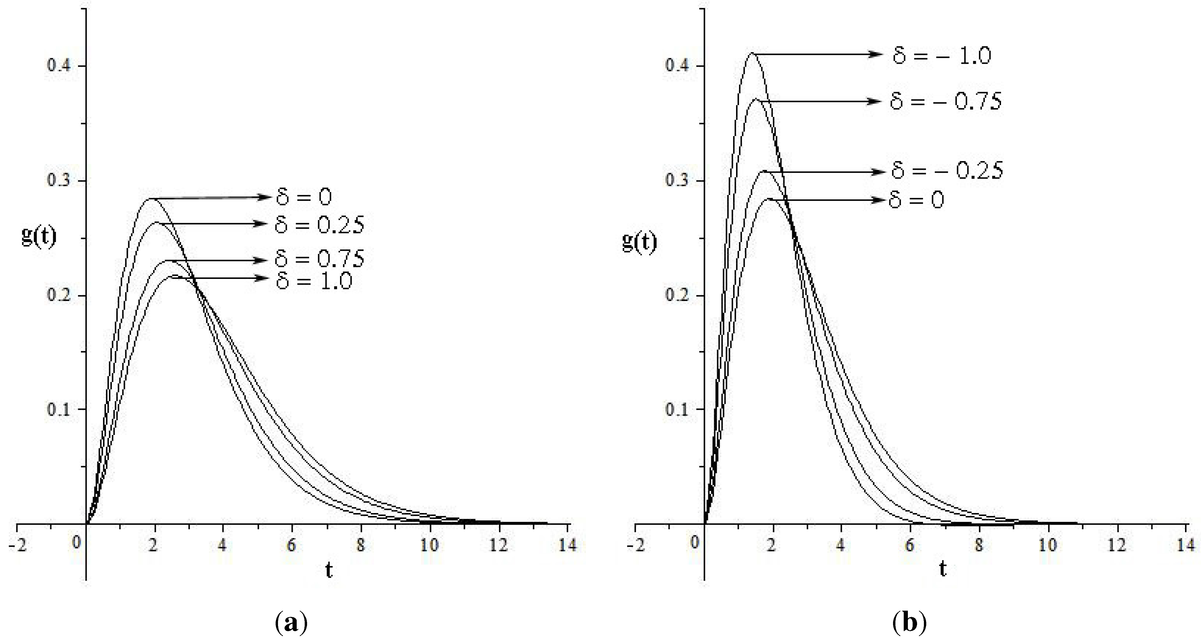
4. Applications in Statistical Mechanics

Nonequilibrium complex systems often exhibit dynamics that can be decomposed into several dynamics on different time scales. As a simple example, consider a Brownian motion of a particle moving through a changing fluid environment, characterized by temperature variations on a large scale. In this case, two dynamics are relevant: one is a fast dynamics describing the local motion of the Brownian particle, and the other one is a slow one due to the large global variations of the environment with spatio-temporal inhomogeneities. These effects produce a superposition of two different statistics, which is referred to as superstatistics. The concept of superstatistics has been introduced by [21,22] after some preliminary considerations in [23,24]. The stationary distributions of superstatistical systems typically exhibit a non-Gaussian behavior with fat tails, which can decay, for example, as a power law, a stretched-exponential law or in an even more complicated way [25]. Essential for this approach is the existence of an intensive variable, say β, which fluctuates on a large spatio-temporal scale.
For the above-mentioned example of a superstatistical Brownian particle, β is the fluctuating inverse temperature of the environment. In general, however, β may also be an effective friction constant, a changing mass parameter, a variable noise strength, the fluctuating energy dissipation in turbulent flows, a fluctuating volatility in finance, an environmental parameter for biological systems, a local variance parameter extracted from a signal, and so on. Superstatistics offers a very general framework for treating nonequilibrium stationary states of such complex systems. After the original work in [21], much effort has been made for further theoretical elaboration; see [26,27]. At the same time, it has also been applied successfully to a variety of systems and phenomena, including hydrodynamic turbulence, pattern formation, cosmic rays, mathematical finance, random matrices and hydro-climatic fluctuations.
From a statistical point of view, the procedure is equivalent to starting with a conditional distribution of a gamma type for every given value of a parameter a. Then, a is assumed to have a prior known density of the gamma type. Then, the unconditional density is obtained by integrating out over the density of a. Let us consider the conditional density of the form:
f x | a ( x | a ) = k 1 x γ 1 e a x ρ 0 F 1 ( ; γ ρ ; δ x ρ ) ; 0 x < , ρ , a , γ > 0
and f ( x ) = 0 elsewhere, where k 1 is the normalizing constant. When δ = 0 , Equation (14) reduces to generalized gamma density. Note that this is the generalization of some standard statistical densities, such as gamma, Weibull, exponential, Maxwell–Boltzmann, Rayleigh and many more. When we put ρ = 1 in Equation (14), it reduces to Equation (11). When δ = 0 , ρ = 2 , Equation (14) reduces to folded standard normal density.
Suppose that a has a gamma density given by:
f a ( a ) = λ η a η 1 e λ a Γ ( η ) ; 0 a < , η , λ > 0
and f a ( a ) = 0 elsewhere. In a physical problem, the residual rate of change may have small probabilities of it being too large or too small, and the maximum probability may be for a medium range of values for the residual rate of change a. This is a reasonable assumption. Then, the unconditional density of x is given by:
f x ( x ) = a f x | a ( x | a ) f a ( a ) d a = ρ λ η x γ 1 Γ ( γ ρ ) Γ ( η ) 0 F 1 ( ; γ ρ ; δ x ρ ) I 11
where:
I 11 = 0 a γ ρ + η 1 e a ( λ + x ρ ) δ a d a
Note that one form of the inverse Gaussian probability density function is given by:
h 1 ( x ) = c x 3 2 e ξ 2 [ x ν 2 + 1 x ] , ν 0 , ξ > 0 , x 0
where c is the normalizing constant. Put γ ρ + η 1 = 3 2 , λ + x ρ = ξ 2 ν 2 , δ = ξ 2 in I 11 ; we can see that the inverse Gaussian density is the integrand in I 11 . Hence, I 11 can be used to evaluate the moments of inverse Gaussian density. Furthermore, I 11 is the special case of the reaction rate probability integral in nuclear reaction rate theory, Krätzel integrals in applied analysis, etc. (see [28,29,30,31]). For the evaluation of this integral and for more details, see [19,20]. Hence, we have the unconditional density:
f x ( x ) = ρ λ η Γ ( γ ρ ) Γ ( η ) x γ 1 ( λ + x ρ ) γ ρ + η 0 F 1 ( ; γ ρ ; δ x ρ ) G 0 , 2 2 , 0 [ δ ( λ + x ρ ) | 0 , γ ρ + η ]
where the G-function is defined as the following Mellin–Barnes integral:
G p , q m , n z | b 1 , , b q a 1 , , a p = 1 2 π i L Φ ( s ) z s d s
where:
Φ ( s ) = j = 1 m Γ ( b j + s ) j = 1 n Γ ( 1 a j s ) j = m + 1 q Γ ( 1 b j s ) j = n + 1 p Γ ( a j + s )
with a j , j = 1 , , p and b j , j = 1 , , q being complex numbers and L a contour separating the poles of Γ ( b j + s ) , j = 1 , , m from those of Γ ( 1 a j s ) , j = 1 , , n . Convergence conditions, properties and applications of the G-function in various disciplines are available in the literature. For example, see [7]. Equation (18) is a superstatistics, in the sense of superimposing another distribution or the distribution of x with superimposed distribution of the parameter a . In a physical problem, the parameter may be something like temperature having its own distribution. Several physical interpretations of superstatistics are available from the papers of Beck and others.
We can easily obtain the series representation of the unconditional density Equation (18), given by:
f x ( x ) = ρ λ η Γ ( γ ρ ) Γ ( η ) x γ 1 ( λ + x ρ ) γ ρ + η 0 F 1 ( ; γ ρ ; δ x ρ ) k = 0 Γ ( γ ρ + η k ) ( 1 ) k [ δ ( λ + x ρ ) ] k k ! = ρ Γ ( γ ρ + η ) λ η Γ ( γ ρ ) Γ ( η ) x γ 1 ( λ + x ρ ) γ ρ + η 0 F 1 ( ; γ ρ ; δ x ρ ) 0 F 1 ( ; 1 γ ρ η ; δ ( λ + x ρ ) ) λ , ρ , η , δ > 0 , γ ρ > 0 , 1 γ ρ η ν , ν = 0 , 1 , , x 0
This series representation provides an extension of the Beck and Cohen statistic. Thus, Equation (19) gives a suitable interpretation, when tail areas are shifted. This model has wide potential applications in physical sciences, especially in statistical mechanics; see [19,20].

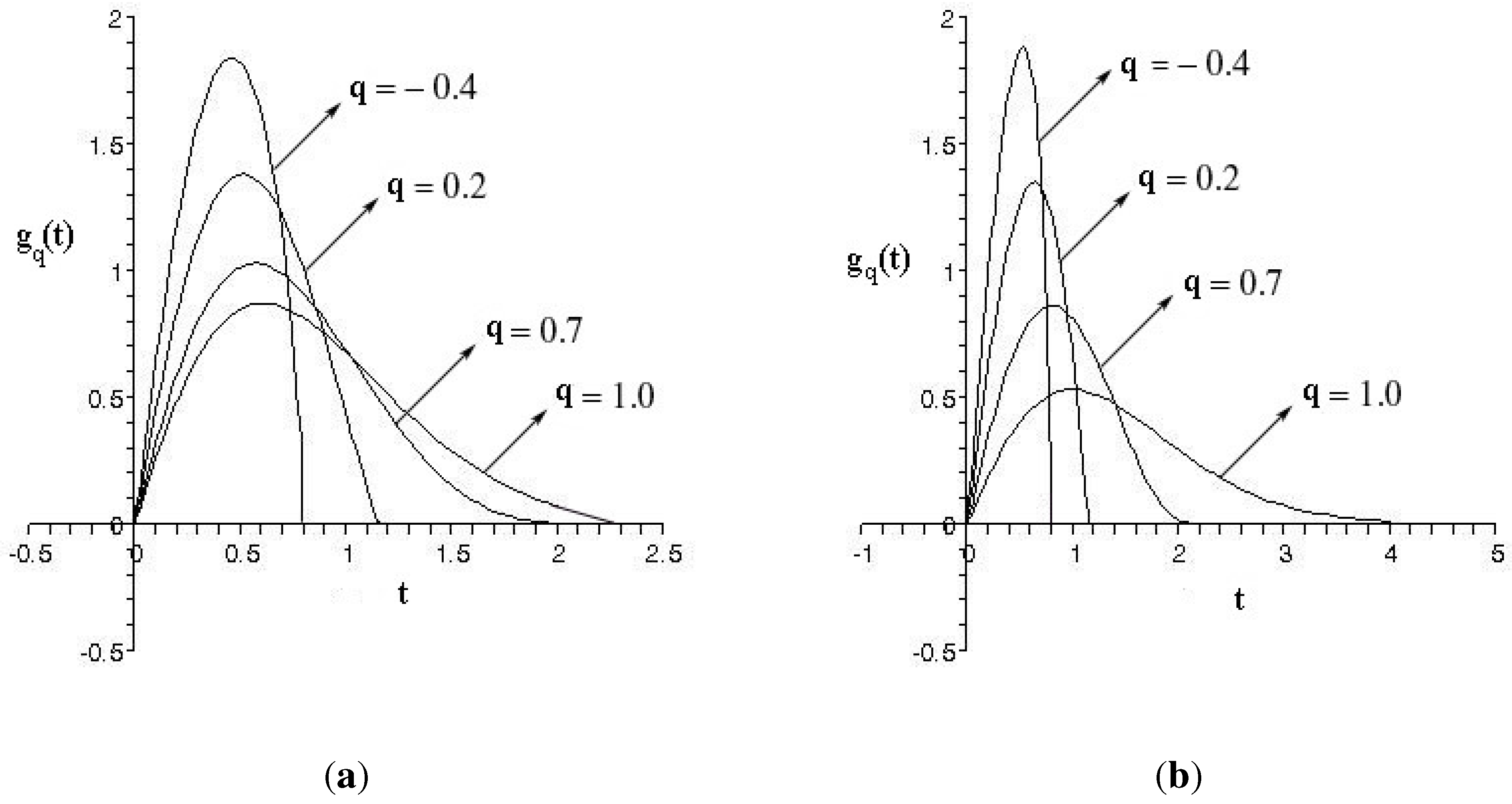
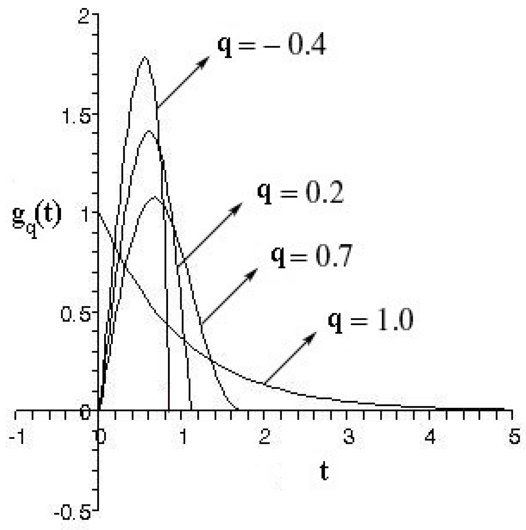
5. Applications in the Growth-Decay Mechanism

If x is replaced by | x | in Equation (3) and when q 1 , the real scalar case of the pathway model takes the form,
h 4 ( x ) = c 4 | x | γ 1 e a | x | θ , < x < , a > 0
The density in Equation (20) for γ = 1 , θ = 1 is the simple Laplace density. For γ = 1 , we have the symmetric Laplace density. A general Laplace density is associated with the concept of the Laplacianness of quadratic and bilinear forms. For the concept of the Laplacianness of bilinear forms, corresponding to the chi-squaredness of quadratic forms, and for other details, see [14,32]. Laplace density is also connected to input-output-type models. Such models can describe many of the phenomena in nature. When two particles react with each other and energy is produced, part of it may be consumed or converted or lost, and what is usually measured is the residual effect. The water storage in a dam at a given instant is the residual effect of the water flowing into the dam minus the amount taken out of the dam. Grain storage in a silo is the input minus the grain taken out. Hence, it is of great importance in modeling this residual effect, and there are many studies on this concept. There are several input-output-type situations in economics, social sciences, industrial production, commercial activities, cosmological studies, and so on. It is shown in [33] that when we have independently-distributed gamma-type input and gamma-type output, the residual part z = x y , x = input variable, y = output variable, then the special cases of the density of z is a Laplace density. In this case, one can also obtain the asymmetric Laplace and generalized Laplace densities, which are currently used very frequently in stochastic processes, as special cases of the input-output model.
The generalized gamma Bessel model in Equation (11) has the moment generating function:
M x ( t ) = b β 1 e δ 1 b e δ 1 b t ( a 1 t ) β 1 , b t > 0 , β 1 > 0
Let x and y be two independently-distributed generalized gamma Bessel models having parameters ( α 1 , β 1 , δ 1 ) and ( α 2 , β 2 , δ 2 ) , respectively, α i > 0 , β i > 0 , δ i , i = 1 , 2 . Let z = x y . Due to the independence of x and y, the moment-generating function of u is given by:
M z ( t ) = α 1 β 1 e δ 1 α 1 e δ 1 α 1 t ( α 1 t ) β 1 α 2 β 2 e δ 2 α 2 e δ 2 α 2 + t ( α 2 + t ) β 2 , α 1 t > 0 , α 2 + t > 0
when α 1 = α 2 = α , β 1 = β 2 = β , δ 1 = δ 2 = δ = 0 , then the above equation reduces to that of the generalized Laplacian model of Mathai.

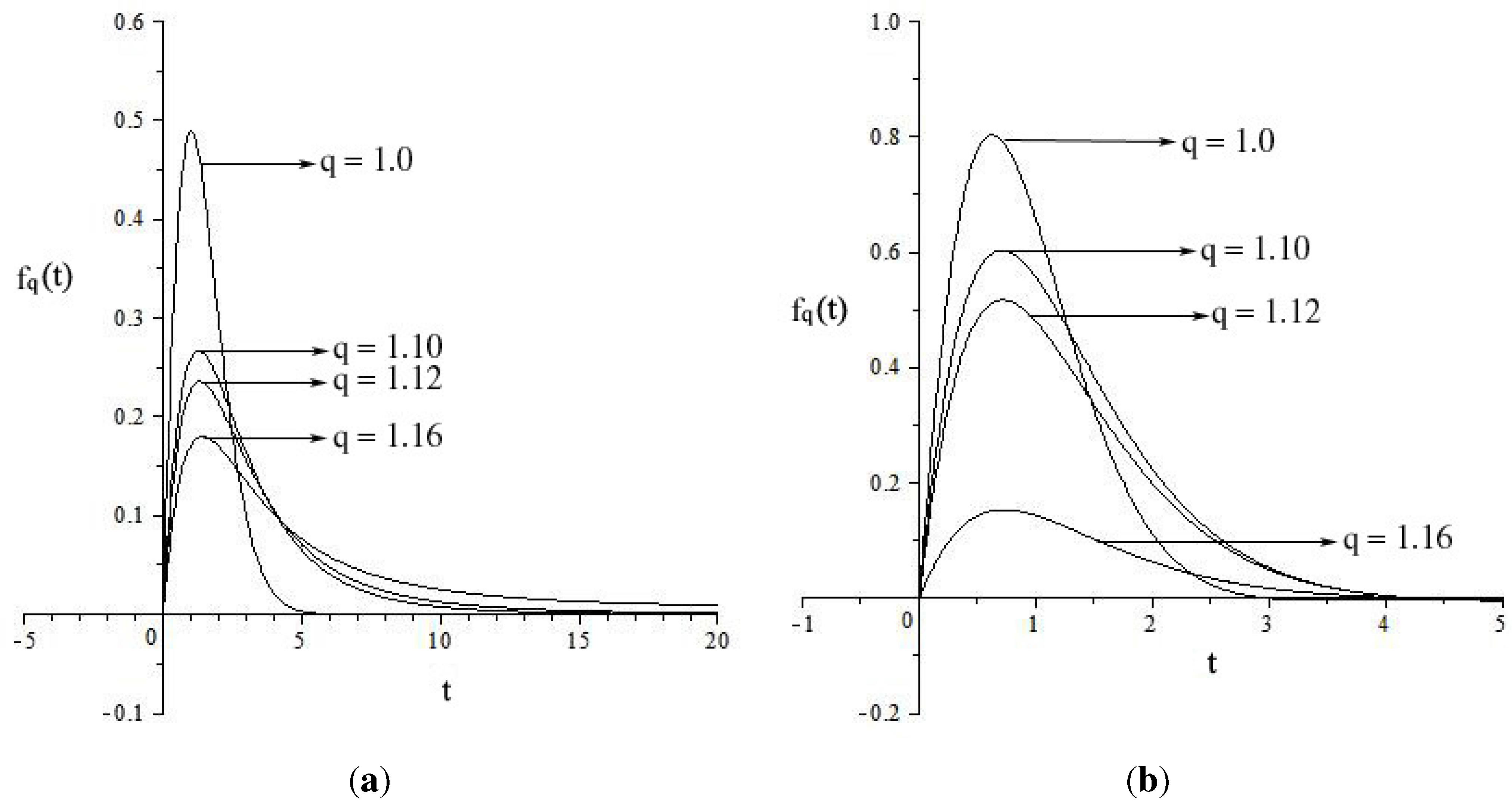
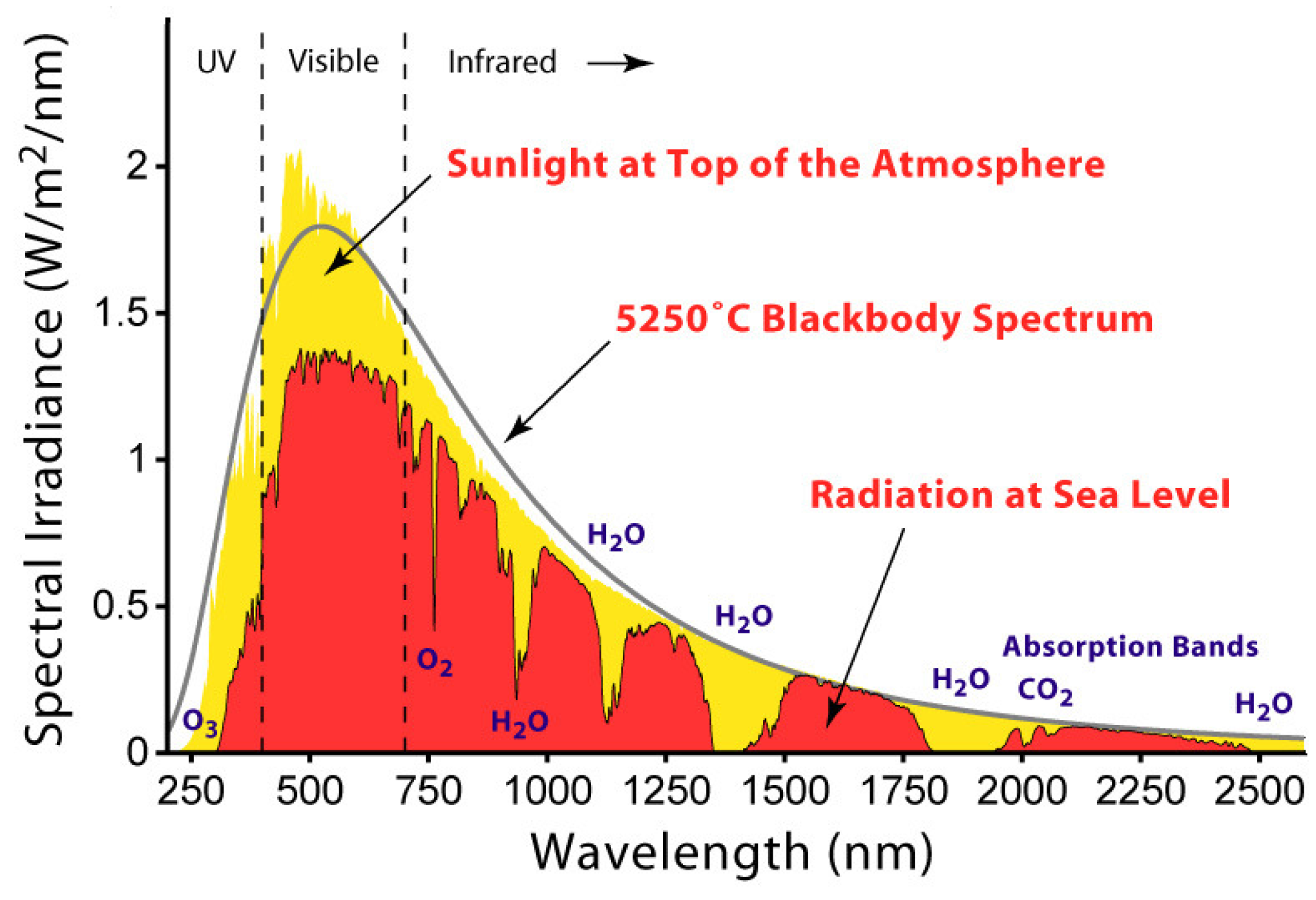
6. Applications in Solar Spectral Irradiance Modeling

Any object with a temperature above absolute zero emits radiation. The Sun, our singular source of renewable energy, sits at the center of the solar system and emits energy as electromagnetic radiation at an extremely large and relatively constant rate, 24 h per day, 365 days of the year. With an effective temperature of approximately 6000 K, the Sun emits radiation over a wide range of wavelengths, commonly labeled from high energy shorter wavelengths to lower energy longer wavelengths as gamma ray, X-ray, ultraviolet, visible, infrared and radio waves. These are called spectral regions; see Figure 5. The rate at which solar energy reaches a unit area at the Earth is called the “solar irradiance” or “insolation”. The units of measure for irradiance are watts per square meter (W/m 2 ). Solar irradiance is an instantaneous measure of rate and can vary over time. The units of measure for solar radiation are joules per square meter (J/m 2 ), but often watt-hours per square meter (Wh/m 2 ) are used. As will be described above, solar radiation is simply the integration or summation of solar irradiance over a time period. For more details, see [34,35].
Figure 5. Solar irradiance spectrum above the atmosphere and at the surface prepared by Robert A. Rohde (used by copyright from http://www.globalwarmingart.com/wiki/File:Solar- Spectrum-png).
Axioms 04 00385 g005
Good quality, reliable solar radiation data are becoming increasingly important in the field of renewable energy, with regard to both photovoltaic and thermal systems. It helps well-founded decision making on activities, such as research and development, production quality control, determination of optimum locations, monitoring the efficiency of installed systems and predicting the system output under various sky conditions. Especially with larger solar power plants, errors of a few percent can significantly impact the return on investment. Scientists studying climate change are interested in understanding the effects of variations in the total and spectral solar irradiance on Earth and its climate.
A recent set of typical meteorological year (TMY) datasets for the United States, called TMY2 datasets, has been derived from the 30-year historical National Solar Radiation Data Base. In 2000, the American Society for Testing and Materials developed an AM0 reference spectrum (ASTM E-490) for use by the aerospace community. That ASTM E490 Air Mass Zero solar spectral irradiance is based on data from satellites, space shuttle missions, high-altitude aircraft, rocket soundings, ground-based solar telescopes and modeled spectral irradiance. Our dataset consists of 1522 observations collected from http://rredc.nrel.gov/solar/spectra/am0/. Here, mathematical software MAPLE and MATLAB are used for the data analysis. The model considered here is the density function given in Equation (11). In many situations, the gamma model is used to model the spectral density. Figure 6 is the histogram of the data embedded with gamma and our new probability models. We have not specified any parameters here to plot the function. The same program generated the two different graphs as shown below. We calculated the Kolmogorov–Smirnov test statistic for the two different probability models. For gamma density, the value of the statistic is obtained as 0.11139, and for our new probability model, the value is 0.10808. From the table, the value obtained is 0.410. We can see that the two different probability models are consistent with the data. However, the distance measure of the statistic of our new probability model is less than the other probability model, and hence, our model is better fit to the data than the other one.
Figure 6. The graph of the histogram embedded with the probability models.
Axioms 04 00385 g006

Acknowledgments

The author acknowledges gratefully the encouragement given by Arak M. Mathai, Department of Mathematics and Statistics, McGill University, Montreal H3A 2K6, Canada.

Conflicts of Interest

The authors declare no conflict of interest.

References

  1. Haubold, H.J.; Mathai, A.M. The fractional kinetic equation and thermonuclear functions. Astrophys. Space Sci. 2000, 273, 53–63. [Google Scholar] [CrossRef]
  2. Henry, B.I.; Wearne, S.L. Existence of Turing instabilities in a two-species fractional reaction-diffusion system. SIAM J. Appl. Math. 2002, 62, 870–887. [Google Scholar] [CrossRef]
  3. Kilbas, A.A.; Saigo, M.; Saxena, R.K. Generalized Mittag-Leffler function and generalized fractional calculus operators. Integral Transform. Special Funct. 2004, 15, 31–49. [Google Scholar] [CrossRef]
  4. Mainardi, F.; Luchko, Y.; Pagnini, G. The fundamental solution of the space-time fractional diffusion equation. Fract. Calc. Appl. Anal. 2001, 4, 153–192. [Google Scholar]
  5. Mathai, A.M.; Haubold, H.J. Pathway model, superstatistics, Tsallis statistics and a generalized measure of entropy. Phys. A 2007, 375, 110–122. [Google Scholar] [CrossRef]
  6. Saxena, R.K.; Mathai, A.M.; Haubold, H.J. Fractional reaction-diffusion equations. Astrophys. Space Sci. 2006, 305, 289–296. [Google Scholar] [CrossRef]
  7. Kilbas, A.A.; Saigo, M. H-Transforms: Theory and Applications; CRC Press: New York, NY, USA, 2004. [Google Scholar]
  8. Kiryakova, V. Generalized Fractional Calculus and Applications; CRC Press: New York, NY, USA, 1994. [Google Scholar]
  9. Miller, K.S.; Ross, B. An Introduction to the Fractional Calculus and Fractional Differential Equations; Wiley: New York, NY, USA, 1993. [Google Scholar]
  10. Podlubny, I. Fractional Differential Equations; Academic Press: San Diego, CA, USA, 1999. [Google Scholar]
  11. Samko, S.G.; Kilbas, A.A.; Marichev, O.I. Fractional Integrals and Derivatives: Theory and Applications; Gordon and Breach: New York, NY, USA, 1990. [Google Scholar]
  12. Mathai, A.M. A pathway to matrix-variate gamma and normal densities. Linear Algebra Its Appl. 2005, 396, 317–328. [Google Scholar] [CrossRef]
  13. Honerkamp, J. Stochastic Dynamical Systems: Concepts, Numerical Methods, Data Analysis; VCH Publishers: New York, NY, USA, 1994. [Google Scholar]
  14. Mathai, A.M. On non-central generalized Laplacianness of quadratic forms in normal variables. J. Multivar. Anal. 1993, 45, 239–246. [Google Scholar] [CrossRef]
  15. Nair, S.S. Pathway fractinal integration operator. Fract. Calc. Appl. Anal. 2009, 12, 237–252. [Google Scholar]
  16. Mathai, A.M. Fractional integrals in the matrix-variate cases and connection to statistical distributions. Integral Transform. Special Funct. 2009, 20, 871–882. [Google Scholar] [CrossRef]
  17. Nair, S.S. Pathway fractional integral operator and matrix-variate functions. Integral Transform. Special Funct. 2011, 22, 233–244. [Google Scholar] [CrossRef]
  18. Sebastian, N. Some statistical aspects of fractional calculus. J. Kerala Stat. Assoc. 2009, 20, 23–33. [Google Scholar]
  19. Sebastian, N. A generalized gamma model associated with Bessel function and its applications in statistical mechanics. In Proceedings of AMADE-09, Proceedings of Institute of Mathematics, Natinal Academy of Sciences, Minsk, Belarus; 2009; pp. 114–119. [Google Scholar]
  20. Sebastian, N. A generalized gamma model associated with a Bessel function. Integral Transform. Special Funct. 2011, 22, 631–645. [Google Scholar] [CrossRef]
  21. Beck, C.; Cohen, E.G.D. Superstatistics. Phys. A 2003, 322, 267–275. [Google Scholar] [CrossRef]
  22. Beck, C. Stretched exponentials from superstatistics. Phys. A 2006, 365, 96–101. [Google Scholar] [CrossRef]
  23. Beck, C. Dynamical Foundations of Nonextensive Statistical Mechanics. Phys. Rev. Lett. 2001, 87, 180601. [Google Scholar] [CrossRef]
  24. Beck, C. Non-additivity of Tsallis entropies and fluctuations of temperature. Europhys. Lett. 2002, 57, 329–333. [Google Scholar] [CrossRef]
  25. Touchette, H. Nonextensive Entropy-Interdisciplinary Applications; Gell-Mann, M., Tsallis, C., Eds.; Oxford University Press: Oxford, UK, 2004. [Google Scholar]
  26. Beck, C. Comment on critique of q-entropy for thermal statistics. Phys. Rev. E 2004, 69, 038101. [Google Scholar]
  27. Chavanis, P.H. Coarse-grained distributions and superstatistics. Phys. A 2006, 359, 177–212. [Google Scholar] [CrossRef]
  28. Joseph, D.P. Gamma distribution and extensions using pathway idea. Stat. Pap. 2011, 52, 309–325. [Google Scholar] [CrossRef]
  29. Krätzel, E. Integral transformations of Bessel type. 1979; 148–155. [Google Scholar]
  30. Mathai, A.M.; Haubold, H.J. Mordern Problems in Nuclear and Neutrino Astrophysics; Akademie-Verlag: Berlin, Germany, 1988. [Google Scholar]
  31. Mathai, A.M. A Versatile Integral. CMS Project SR/S4/MS:287/05. Preprint. 2007; 9. [Google Scholar]
  32. Mathai, A.M.; Provost, S.B.; Hayakawa, T. Bilinear Forms and Zonal Polynomials; Lecture notes in Statistics, No. 102; Springer-Verlag: New York, MY, USA, 1995. [Google Scholar]
  33. Mathai, A.M. The residual effect of growth-decay mechanism and the distributions of covariance structure. Can. J. Stat. 1993, 21, 277–283. [Google Scholar] [CrossRef]
  34. Gueymard, C. The sun’s total and spectral irradiance for solar energy applications and solar radiation models. Sol. Energy 2004, 76, 423–453. [Google Scholar] [CrossRef]
  35. Stoffel, T.; Renné, D.; Myers, D.; Wilcox, S.; Sengupta, M.; George, R.; Turchi, C. Concentrating Solar Power. Available online: http://www.nrel.gov/docs/fy10osti/47465.pdf (accessed on 13 August 2015).

