Diffeomorphism Spline

Abstract

Conventional splines offer powerful means for modeling surfaces and volumes in three-dimensional Euclidean space. A one-dimensional quaternion spline has been applied for animation purpose, where the splines are defined to model a one-dimensional submanifold in the three-dimensional Lie group. Given two surfaces, all of the diffeomorphisms between them form an infinite dimensional manifold, the so-called diffeomorphism space. In this work, we propose a novel scheme to model finite dimensional submanifolds in the diffeomorphism space by generalizing conventional splines. According to quasiconformal geometry theorem, each diffeomorphism determines a Beltrami differential on the source surface. Inversely, the diffeomorphism is determined by its Beltrami differential with normalization conditions. Therefore, the diffeomorphism space has one-to-one correspondence to the space of a special differential form. The convex combination of Beltrami differentials is still a Beltrami differential. Therefore, the conventional spline scheme can be generalized to the Beltrami differential space and, consequently, to the diffeomorphism space. Our experiments demonstrate the efficiency and efficacy of diffeomorphism splines. The diffeomorphism spline has many potential applications, such as surface registration, tracking and animation.

1. Introduction

Conventional splines are applied for modeling shapes [1,2,3,4,5,6,7]. For example, spline curves are used to model planar curves; bi-variant splines are applied for modeling geometric surfaces embedded in ${\mathbb{R}}^3$; and tri-variant splines are used for volumes. Basically, a m-variate spline can be viewed as a mapping $\gamma :\mathsf{\Omega }\to {\mathbb{R}}^n$, where $\mathsf{\Omega }\subset {\mathbb{R}}^m$ is the parameter domain. The target space ${\mathbb{R}}^n$ can be replaced by an abstract manifold $M^n$, as long as the convex linear combination of two points is well defined in $M^n$.

In the graphics field, quaternion splines [8] have been applied for key frame animation purposes. Quaternions are the representation of rotations in ${\mathbb{R}}^3$. The rotation group, denoted as $SO\left(3\right)$, is a Lie group, which has a natural Riemannian metric. Given two quaternions $q_1,q_2\in SO\left(3\right)$, there exists a unique geodesic connecting them. Suppose q is the linear interpolation between $q_1,q_2$ with ratio λ, then q is on the geodesic, and $\frac{d(q,q_1)}{d(q_1,q_2)}=1-\lambda ,$ where d represents the geodesic distance between two quaternions. Based on the linear interpolation of quaternions, the quaternion spline can be defined using de Casteljau’s evaluation algorithm [3]. The quaternion spline is a commonly-used spline, which is defined in a finite dimensional Lie group.

In this work, we aim at defining spline schemes in an infinite dimensional space, the diffeomorphism space, which is formed by all diffeomorphisms between surfaces. In mathematics, a diffeomorphism is an isomorphism of smooth manifolds. It is an invertible function that maps one differentiable manifold to another, such that both the function and its inverse are smooth. Figure 1 shows a diffeomorphism of an image. The distortions are visualized by the shape change of circles.

Figure 1. A diffeomorphism of an image caused by a quasiconformal mapping. The distortion of circles demonstrates the diffeomorphism of the original image. (a) Original image; (b) deformed image; (c) quasiconformal deformation.

Figure 1. A diffeomorphism of an image caused by a quasiconformal mapping. The distortion of circles demonstrates the diffeomorphism of the original image. (a) Original image; (b) deformed image; (c) quasiconformal deformation.

Generally speaking, suppose $S_1,S_2$ are two surfaces in ${\mathbb{R}}^3$, and $f,g:S_1\to S_2$ are two mappings. For a point $p\in S_1$, the linear combination of its images $f\left(p\right),g\left(p\right)\in S_2$, $\lambda f\left(p\right)+(1-\lambda )g\left(p\right),\lambda \in \mathbb{R}$, may not be on $S_2$. Even if for all points on $S_1$, the linear combinations of its images are on $S_2$, the mapping $\lambda f+(1-\lambda )g$ may not be a diffeomorphism. This means that direct linear interpolation of diffeomorphisms cannot guarantee a diffeomorphism. This causes the intrinsic difficulty to define splines in diffeomorphism space.

1.1. Approach Overview

The solution to solve the problem is to convert the diffeomorphism space into a functional space, where each point is a function and uniquely determines a diffeomorphism. The definition of this function is based on the canonical conformal (angle preserving) parameterizations of the source and target surfaces. The diffeomorphisms between these two surfaces are converted to the ones between their parameter domains. Once we have the diffeomorphisms, we compute their associated functions and use them to construct a spline in the infinite dimensional functional space to interpolate diffeomorphisms. The proposed solution can handle general surfaces. For the sake of simplicity, we assume that $S_1$ and $S_2$ are genus zero surfaces with a single boundary component, such as human face surfaces. In detail, the computing strategy is as follows:

First, we convert the mapping space to a functional space. There exist conformal (angle preserving) mappings ${\varphi }_k:S_k\to \mathbb{D}$, where $\mathbb{D}$ is the unit disk on the complex plane, $\mathbb{D}=\left\{\right|z|<1|z\in \mathbb{C}\}$. Any diffeomorphism $\varphi :S_1\to S_2$ corresponds to an automorphism ${\varphi }_2\circ \varphi \circ {\varphi }_1^{-1}:\mathbb{D}\to \mathbb{D}.$ Therefore, the diffeomorphism space between $S_1$ and $S_2$ is equivalent to the automorphism group of $\mathbb{D}$, $Aut\left(\mathbb{D}\right)$. We define the normalized automorphism group of $\mathbb{D}$, $\overline{Aut}\left(\mathbb{D}\right)$, as $\overline{Aut}\left(\mathbb{D}\right)=\{f\in Aut\left(\mathbb{D}\right)|f\left(0\right)=0,f\left(1\right)=1\}.$ Let $f\in Aut\left(\mathbb{D}\right)$, then the Beltrami coefficient of f is a complex valued function, given by:

$${\mu }_f\left(z\right)=\frac{f_{\overline{z}}}{f_z}\left(z\right)$$

By direct computation, $\parallel {\mu }_f{\parallel }_{\infty }=su{p}_{z\in \mathbb{D}}\parallel {\mu }_f\left(z\right)\parallel <1.$ In the general manifold setting, the Beltrami coefficient is generalized to the Beltrami differential [9]. Furthermore, we show that for two normalized mappings $f_1,f_2\in \overline{Aut}\left(\mathbb{D}\right)$, if ${\mu }_{f_1}={\mu }_{f_2}$, then $f_1=f_2$, and any μ with ${\parallel \mu \parallel }_{\infty }<1$ must be the Beltrami coefficient of a normalized automorphism $f\in \overline{Aut}\left(\mathbb{D}\right)$. Namely,

$$\overline{Aut}{\left(\mathbb{D}\right)\cong \left\{\mu \right|\parallel \mu \parallel }_{\infty }<1,\mu :\mathbb{D}\to \mathbb{C}\}$$

Next, we define the linear interpolation between two automorphisms and that between two mappings. Suppose $f,g\in \overline{Aut}\left(\mathbb{D}\right)$ are two normalized automorphisms. Choose a $\lambda \in [0,1]$ and define ${\mu }_{\lambda }:=(1-\lambda ){\mu }_f+\lambda {\mu }_g$, then:

$$\parallel {\mu }_{\lambda }{\parallel }_{\infty }\le (1-\lambda )\parallel {\mu }_f{\parallel }_{\infty }+\lambda {\parallel {\mu }_g\parallel }_{\infty }<1$$

There exists a unique ${\varphi }_{\lambda }$ whose Beltrami coefficient equals ${\mu }_{\lambda }$. Then, ${\varphi }_{\lambda }$ is the linear interpolation between f and g with ratio λ. Suppose $f,g:S_1\to S_2$ are two mappings between surfaces. By applying the conformal mappings ${\varphi }_k:S_k\to \mathbb{D}$, ${\varphi }_2\circ f\circ {\varphi }_1^{-1}$ and ${\varphi }_2\circ g\circ {\varphi }_1^{-1}$ become automorphisms of the unit disk. Suppose ${\varphi }_{\lambda }$ is the linear interpolation between them, then ${\varphi }_2^{-1}\circ {\varphi }_{\lambda }\circ {\varphi }_1:S_1\to S_2$ is the linear interpolation between the original f and g.

Then, we define the spline curve in the diffeomorphism space from $S_1$ to $S_2$ using de Casteljau’s evaluation algorithm [3]. By using tensor product construction, multiple variant (m-variant) diffeomorphism splines can be defined accordingly.

In summary, we first convert the space of all the diffeomorphisms from $S_1$ to $S_2$ to the complex functional space on $S_1$, the so-called Beltrami coefficient space. The Beltrami coefficient space is closed under a convex linear combination operation. Therefore, we define splines in the Beltrami coefficient space, and each point on the Beltrami coefficient spline corresponds to a diffeomorphism. In this way, we define the splines in the diffeomorphism space.

1.2. Potential Applications

The diffeomorphism spline has many applications. It can be directly applied for animation purposes. A 2D animation can be treated as a time-dependent mapping $f\left(t\right):{\mathsf{\Omega }}_1\to {\mathsf{\Omega }}_2$; both ${\mathsf{\Omega }}_1$ and ${\mathsf{\Omega }}_2$ are planar domains; ${\mathsf{\Omega }}_1$ represents the static texture; ${\mathsf{\Omega }}_2$ represents the image plane. By changing the mapping $f\left(t\right)$, the 2D texture ${\mathsf{\Omega }}_1$ is animated on the image plane ${\mathsf{\Omega }}_2$. The animator only specifies several key frames of the mapping $f\left(t\right)$, as the control points $\{f\left(t_0\right),f\left(t_1\right),\cdots ,f\left(t_m\right)\}$. By using the diffeomorphism spline, we can generate a smooth sequence of mappings $f\left(t\right)$.

Another application is 3D deformable tracking. With the development of 3D scanning techniques, a high-speed 3D scanner can capture 3D dynamic surfaces in real time [10], such as a human expression sequence. The frames in the sequence are independent of each other. It is highly desirable to establish the correspondence among all of the frames, which is called the 3D tracking problem. We tackle the problem using our diffeomorphism spline technique. First, each frame $S\left(t\right)$ is conformally mapped to the unit disk $\mathbb{D}$ with normalization conditions. Then, the mapping from the first frame to the frame at time t, $f\left(t\right):S\left(0\right)\to S\left(t\right)$, is in $\overline{Aut}\left(\mathbb{D}\right)$. We only compute a few key mappings $\{f\left(t_0\right),f\left(t_1\right),\cdots ,f\left(t_m\right)\}$ as control points and construct the diffeomorphism spline. The spline gives the registration and tracking results without computing all of the mappings for each frame.

1.3. Related Works

There are some existing methods searching for optimal diffeomorphisms, such as curvature representations [11], regional point representations [12,13], spherical harmonic representations [14,15], shape distributions [16], physics-based deformable models [17], free-form deformation (FFD) [18] and level-set methods [19]. FFD embeds the surface in a volume, by deforming the volume to match surfaces. This method minimizes a special energy using the explicit embedding. Similarly, the deformation field method optimizes the matching energy, and the variation gives the deformation field. These methods may encounter local extremes and cannot guarantee global optimization, especially for deformable non-rigid surfaces with significantly non-rigid deformation, even if the deformations are isometric.

Surface conformal mapping-based methods have been developed for surface matching [20,21,22], registration [23,24] and tracking [25]. The key idea is to map surfaces to 2D canonical domains and then solve the surface registration problem as an image registration problem. The conformal mapping-based methods can handle nonrigid deformations between surfaces. Surface conformal mapping can be generalized to surface quasiconformal mapping, which has great potential to handle large-scale nonrigid (including non-isometric) deformations in surface registration applications. The Beltrami holomorphic flow method [26] and the auxiliary metric method [27] were introduced for computing surface quasiconformal maps and have been used for surface registration, compression and inpainting [28,29]. Simple formulas were given in [30] for computing quasiconformal plane deformations. Extremal quasiconformal maps between two planar disks with Dirichlet boundary conditions were recently explored in [31] for computing surface parameterization.

A series of experiments have been conducted to verify whether natural surface deformations are conformal or not [32]. In the real physical world, isometric or even conformal mappings are rare. Most natural deformations in the physical world are quasiconformal. The surface registration and tracking methods based on quasiconformal mappings [27] searching in the diffeomorphism group can model almost all natural physical deformations. The methods searching in the rigid motion, isometry or conformal transformation group are subsumed by the method based on quasiconformal mappings. If the optimal solution is a conformal mapping, the method can find it. Therefore, the method in the diffeomorphism category is more desirable to handle large deformations in practice.

2. Mathematical Background

In this section, we briefly introduce the most related mathematical background. For a comprehensive treatment and for references to the extensive literature on the subject, one may refer to [9] for quasiconformal geometry, [33] for complex analysis and [34] for the Riemann surface.

2.1. Beltrami Coefficient

Suppose $f\left(z\right):\mathbb{C}\to \mathbb{C}$ is a complex valued function on the complex plane; its real representation is $f(x+iy)=u(x,y)+iv(x,y)$. The complex differential operators are defined as:

$$\frac{\partial }{\partial z}=\frac{1}{2}(\frac{\partial }{\partial x}-i\frac{\partial }{\partial y}),\frac{\partial }{\partial \overline{z}}=\frac{1}{2}(\frac{\partial }{\partial x}+i\frac{\partial }{\partial y})$$

$f\left(z\right)$ is a conformal map (also called conformal transformation, angle-preserving transformation or biholomorphic map), if and only if $\frac{\partial f}{\partial \overline{z}}=0$, meaning f satisfies the Cauchy–Riemann equations:

$$\frac{\partial u}{\partial x}=\frac{\partial v}{\partial y},\frac{\partial u}{\partial y}=-\frac{\partial v}{\partial x}$$

An analytic (holomorphic) function is conformal at any point where it has a nonzero derivative.

Definition 1 (Beltrami Coefficient). Suppose $f\left(z\right):\mathbb{C}\to \mathbb{C}$ is a complex valued function on the complex plane; it satisfies the following Beltrami equation:

$$\frac{\partial f}{\partial \overline{z}}=\mu \frac{\partial f}{\partial z}$$

(1)

where μ is called the Beltrami coefficient, ${\parallel \mu \parallel }_{\infty }<1$.

If Beltrami coefficient μ is zero, then the mapping is a conformal mapping; otherwise, it is a quasiconformal mapping. The conformal mapping maps infinitesimal circles to infinitesimal circles, while quasiconformal mapping maps infinitesimal ellipses to infinitesimal circles. The eccentricity of the infinitesimal ellipse is described by the dilatation:

$$K\left(z\right)=\frac{1+\left|\mu \right(z\left)\right|}{1-\left|\mu \right(z\left)\right|},K\ge 1$$

(2)

which is the ratio between the longer axis and the shorter axis of the infinitesimal ellipse. The orientation of the infinitesimal is given by:

$$\theta \left(z\right)=\frac{1}{2}arg\mu \left(z\right),\theta \in (-\frac{\pi }{2},\frac{\pi }{2}]$$

(3)

which is the angle between the longer axis and the real axis.

Figure 2 gives the examples on the planar domain to demonstrate quasiconformal deformations. There are six quasiconformal mappings of a square D, $f_i\left(z\right):D\to D,i=1,\dots ,6$, where $f_2$, $f_4$, $f_6$ are the inverse diffeomorphisms of $f_1$, $f_3$, $f_5$, respectively. Each $f_i\left(z\right)$ has an explicit formula; therefore, the Beltrami coefficients μ can be computed explicitly by using Equation (1). Furthermore, all of the functions are symmetric. The distortion of consistent checkers (circles) visualizes the quasiconformality of diffeomorphisms obviously.

Figure 2. Diffeomorphisms of a square. Each diffeomorphism $f_i,i=0,\dots ,6$, is a quasiconformal automorphism of a square D (to itself). The first row shows the consistent checker-board texture mapping results for $f_i$. The second row shows the corresponding circle packing texture mapping results. The distortion of checkers (circles) visualizes the quasiconformality of diffeomorphisms.

Figure 2. Diffeomorphisms of a square. Each diffeomorphism $f_i,i=0,\dots ,6$, is a quasiconformal automorphism of a square D (to itself). The first row shows the consistent checker-board texture mapping results for $f_i$. The second row shows the corresponding circle packing texture mapping results. The distortion of checkers (circles) visualizes the quasiconformality of diffeomorphisms.

2.2. Diffeomorphism

Definition 2 (Diffeomorphism). A bijective map f from $S_1$ to $S_2$ is called a diffeomorphism if both $f:S_1\to S_2$ and its inverse $f^{-1}:S_2\to S_1$ are differentiable.

All diffeomorphisms between two surfaces can be classified by homotopy. In topology, two continuous mappings from one topological space to another are called homotopic if one can be continuously deformed into the other; such a deformation is called a homotopy between the two mappings. If the automorphisms of a surface form a set, then they form a group under the composition of morphisms. This group is called the automorphism group of the surface.

Definition 3 (Automorphism Group). All of the diffeomorphisms from a surface S to itself, which are homotopic to the identity map, form a group. We call it the automorphism group, denoted as $Aut\left(S\right)$.

Note that the diffeomorphisms in the automorphism group are orientation preserving, so that reflections from a surface S to itself are excluded. The automorphism group $Aut\left(S\right)$ is an infinite dimensional Lie group. A m-variate diffeomorphism spline is defined as a smooth mapping $\gamma :\mathsf{\Omega }\to Aut\left(S\right)$, $\mathsf{\Omega }\subset {\mathbb{R}}^m$. Furthermore, the spline is defined by the control points, and each point is a diffeomorphism in diffeomorphism space.

2.3. Quasiconformal Mapping

Suppose $S_1$ and $S_2$ are compact surfaces embedded in ${\mathbb{R}}^3$, then they naturally have induced Euclidean metric ${\mathbf{g}}_1$ and ${\mathbf{g}}_2$. Suppose $\varphi :(S_1,{\mathbf{g}}_1)\to (S_2,{\mathbf{g}}_2)$ is an orientation preserving diffeomorphism between them. We say the mapping ϕ is conformal if it preserves angles; mathematically, the pullback metric ${\varphi }^{*}{\mathbf{g}}_2$ on $S_1$ differs from the original metric ${\mathbf{g}}_1$ by a scalar function,

$${\varphi }^{*}{\mathbf{g}}_2=e^{2\lambda }{\mathbf{g}}_1$$

where $\lambda :S_1\to \mathbb{R}$ is a function. In general, the mapping ϕ does not preserve angles. We say the mapping is quasiconformal, if the distortion between the angle structures induced by ϕ is bounded.

Theorem 4. Suppose $\varphi :(S_1,{\mathbf{g}}_1)\to (S_2,{\mathbf{g}}_2)$ is a diffeomorphism between two compact surfaces, then ϕ is a quasiconformal mapping.

The proof of this theorem requires the concept of Beltrami coefficient μ. In the following, we first consider mappings between domains on the complex plane and then generalize the concept and the method to general surfaces.

2.4. Generalized Riemann Mapping for Planar Domains

All of the conformal mappings of the unit disk are Möbius transformations, $e^{i\theta }\frac{z-z_0}{1-{\overline{z}}_{0}z}$, $\theta \in [0,2\pi )$, $|z_0|<1$. On the unit disk, a Beltrami coefficient determines a quasiconformal mapping uniquely up to a Möbius transformation. The following theorem generalizes the classical Riemann mapping theorem [9] to quasiconformal mappings.

Theorem 5 (Generalized Measurable Riemann Mapping for Planar Domains). Suppose $S\subset \mathbb{C}$ is a compact domain with a smooth boundary, and suppose $\mu :S\to \mathbb{C}$ is a measurable complex function, such that ${\parallel \mu \parallel }_{\infty }<1$, then there exists a diffeomorphism $f:S\to \mathbb{D}$ mapping S to the unit disk $\mathbb{D}$, whose Beltrami coefficient is μ. Two such kinds of diffeomorphisms differ by a Möbius transformation.

This theorem tells us that each Beltrami coefficient determines a quasiconformal mapping uniquely up to a Möbius transformation. On the other hand, each quasiconformal mapping has a Beltrami coefficient. Therefore, by using this theorem, the space of diffeomorphisms between S and $\mathbb{D}$ and the functional space of Beltrami coefficients have the following relation:

$$\frac{Diff(S,\mathbb{D})}{\left\{M\ddot{o}bius\right\}}\cong \left\{\mu \right|\mu :S\to {\mathbb{C},\parallel \mu \parallel }_{\infty }<1\}$$

Thus, the spline of diffeomorphisms can be further constructed in the Beltrami coefficient space, and this theorem guarantees that the Beltrami coefficient resulting from spline interpolation uniquely determines a diffeomorphism up to a Möbius transformation.

2.5. Generalized Riemann Mapping for Surfaces

The generalized Riemann mapping theorem also holds for surfaces. First, the concept of the Beltrami coefficient is generalized to the Beltrami differential. Then, we show that the Beltrami differential uniquely determines the mapping.

2.5.1. Surface Ricci Flow

Ricci flow refers to the process of deforming Riemannian metric $\mathbf{g}$ proportional to the curvature K, such that the curvature evolves according to a heat diffusion process; eventually, the curvature becomes constant everywhere. Analytically, surface Ricci flow is defined as $\frac{d\mathbf{g}}{dt}=-2K\mathbf{g}$. It conformally deforms the Riemannian metric and converges to constant curvature metric [35,36]. This shows the following uniformization theorem [34]:

Theorem 6 (Uniformization). Suppose S is a closed metric surface, then depending on the surface topology, S can be conformally deformed to one of three canonical shapes: the unit sphere ${\mathbb{S}}^2$, the flat torus ${\mathbb{R}}^2/\Gamma$, where Γ is a subgroup of Euclidean translation, or ${\mathbb{H}}^2/\Gamma$, where Γ is a subgroup of a hyperbolic rigid motion group.

This theorem shows that for each metric surface, we can find a conformal atlas $\left\{(U_{\alpha },{\varphi }_{\alpha })\right\}$, such that all of the chart transitions ${\varphi }_{\alpha \beta }:{\varphi }_{\alpha }(U_{\alpha }\cap U_{\beta })\to {\varphi }_{\beta }(U_{\alpha }\cap U_{\beta })$ are the elements in Γ, which are planar conformal mappings. Γ can be the Deck transformation group in the Euclidean domain, the Möbius transformation group on the unit sphere and the Fuchsian transformation group in hyperbolic space. The computational strategies and experimental examples can be found in [37].

2.5.2. Beltrami Differential

Suppose $\varphi :(S_1,{\mathbf{g}}_1)\to (S_2,{\mathbf{g}}_2)$ is an orientation preserving diffeomorphism. The conformal atlases for $S_1,S_2$ are $\left\{(U_{\alpha },{\varphi }_{\alpha })\right\}$ and $\left\{(V_{\beta },{\tau }_{\beta })\right\}$, respectively. If the restriction of the mapping:

$${\tau }_{\beta }\circ \varphi \circ {\varphi }_{\alpha }^{-1}:{\varphi }_{\alpha }\left(U_{\alpha }\right)\to {\tau }_{\beta }\left(V_{\beta }\right)$$

is a quasiconformal mapping on the complex plane, then ϕ is called a quasiconformal mapping.

Definition 7 (Beltrami Differential). Suppose $\left\{(U_{\alpha },{\varphi }_{\alpha })\right\}$ is a conformal atlas of $S_1$, and the local parameters on the chart $(U_{\alpha },{\varphi }_{\alpha })$ is $z_{\alpha }$, then the complex differential is called the Beltrami differential:

$${\mu }_{\alpha }\frac{d{\overline{z}}_{\alpha }}{d{z}_{\alpha }}$$

where ${\mu }_{\alpha }$ is the Beltrami coefficient of the restriction of ϕ on the current local chart ${\tau }_{\beta }\circ \varphi \circ {\varphi }_{\alpha }^{-1}$.

The Beltrami differential is invariant under local parameter change, and it is globally well defined. We have the following theorem [38]:

Theorem 8 (Generalized Measurable Riemann Mapping for Surfaces). Suppose $(S_1,{\mathbf{g}}_1),(S_2,{\mathbf{g}}_2)$ are two compact surfaces with Riemannian metrics. Suppose $\mu \left(z\right)\frac{d\overline{z}}{dz}$ is a measurable complex differential, such that ${\parallel \mu \parallel }_{\infty }<1$; then, there exists a diffeomorphism $\varphi :S_1\to S_2$ mapping $S_1$ to $S_2$, whose Beltrami differential is $\mu \left(z\right)\frac{d\overline{z}}{dz}$.

2.5.3. Auxiliary Metric

A constructive method is given here to solve the Beltrami equation, namely to recover the mapping from its Beltrami differential [38,39]. Suppose $\varphi :\mathsf{\Omega }\to \mathbb{D}$, Ω is in the z-plane and $\mathbb{D}$ is in the w-plane. The Beltrami differential is denoted as $\mu \frac{d\overline{z}}{dz}$. Then:

$$dw\left(z\right)=\frac{\partial w\left(z\right)}{\partial z}dz+\frac{\partial w\left(z\right)}{\partial \overline{z}}d\overline{z}=w_z(dz+\mu d\overline{z})$$

The pullback metric induced by ϕ on Ω is:

$${\varphi }^{*}{\left|dw\right|}^2=|w_z{|}^2{|dz+\mu d\overline{z}|}^2$$

Therefore, the pullback metric is conformal to the auxiliary metric $|dz+\mu d\overline{z}{|}^2$. Namely, we have proven the following theorem:

Theorem 9 (Auxiliary Metric). The quasiconformal map:

$${\varphi :(\mathsf{\Omega },|dz|}^2{)\to (\mathbb{D},\left|dw\right|}^2)$$

becomes a conformal map under the auxiliary metric:

$$\varphi :(\mathsf{\Omega },|dz+\mu d\overline{z}{|}^2{)\to (\mathbb{D},\left|dw\right|}^2)$$

The auxiliary metric is well defined. The proof of this theorem can be found in [38]. It tells us that in order to solve the Beltrami equation on Riemann surfaces, we simply need to define a new auxiliary metric associated with the prescribed Beltrami differential. We can then solve the Beltrami equation by computing a conformal mapping associated with the newly defined metric. In other words, the quasiconformal mapping is equivalent to a conformal mapping under a suitable auxiliary metric.

3. Algorithm

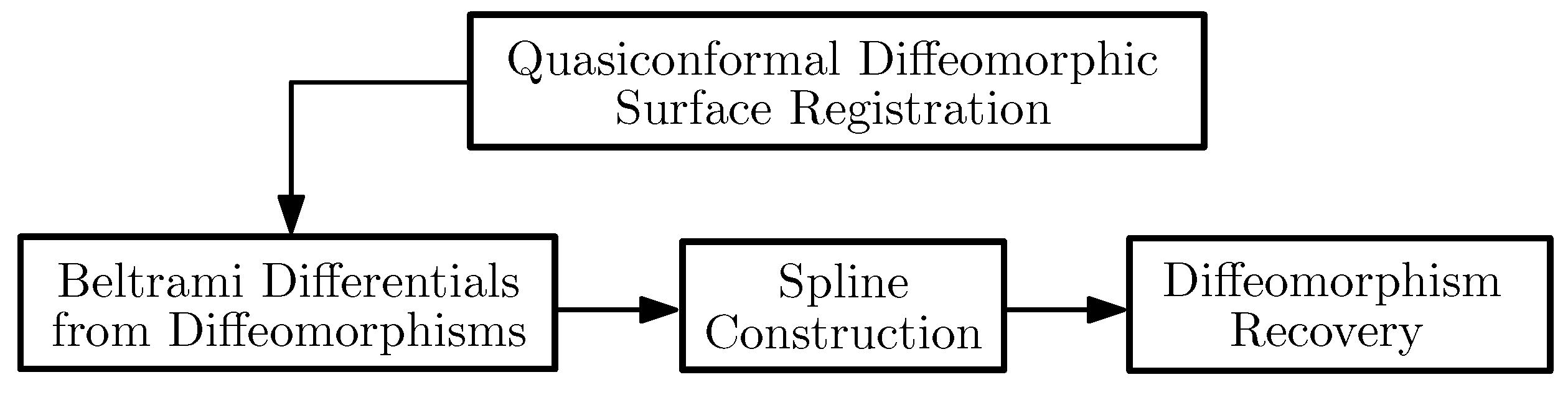
In this section, we explain the computation details for each stage of the pipeline shown in Figure 3. We construct the spline for diffeomorphisms based on conformal mappings and quasiconformal mappings. First, we use conformal mappings to map the surfaces to canonical domains, which provides an efficient approach to deal with 3D problems. Second, we generate diffeomorphisms by the quasiconformal diffeomorphic surface registration method, which operates diffeomorphisms as complex functions, the so-called Beltrami coefficients (Beltrami differentials), and converts diffeomorphism space into a functional space. Third, we apply the Catmull–Rom spline for interpolation between Beltrami differential functions. Each interpolated point corresponds to a diffeomorphism denoted by a Beltrami differential. The diffeomorphism can be recovered by the quasiconformal mapping associated with the interpolated Beltrami differential.

Figure 3. Pipeline for computing the spline of diffeomorphisms.

Figure 3. Pipeline for computing the spline of diffeomorphisms.

3.1. Quasiconformal Diffeomorphic Surface Registration Framework

The surface registration framework is summarized in Diagram (4).

$$\begin{array}{ccc}{S}_1& \stackrel{f}{\to }& S_2\\ {\varphi }_1\downarrow \phantom{{\varphi }_1}& & \phantom{{\varphi }_2}\downarrow {\varphi }_2& & \\ \mathbb{D}& \stackrel{h}{\to }& \mathbb{D}\end{array}$$

(4)

Suppose $S_k,k=1,2$ are the input surfaces. Here, we assume the input surfaces for registration are without occlusions. In order to compute the optimal diffeomorphism $f:S_1\to S_2$ to register them, we conformally map them onto the plane ${\varphi }_k:S_k\to \mathbb{D}$, then construct a planar quasiconformal mapping $h:\mathbb{D}\to \mathbb{D}$; the registration is given by $f={\varphi }_2^{-1}\circ h\circ {\varphi }_1$. The Beltrami coefficient of h is estimated on the planar domain, and h is obtained by solving the Beltrami equation in Equation (1).

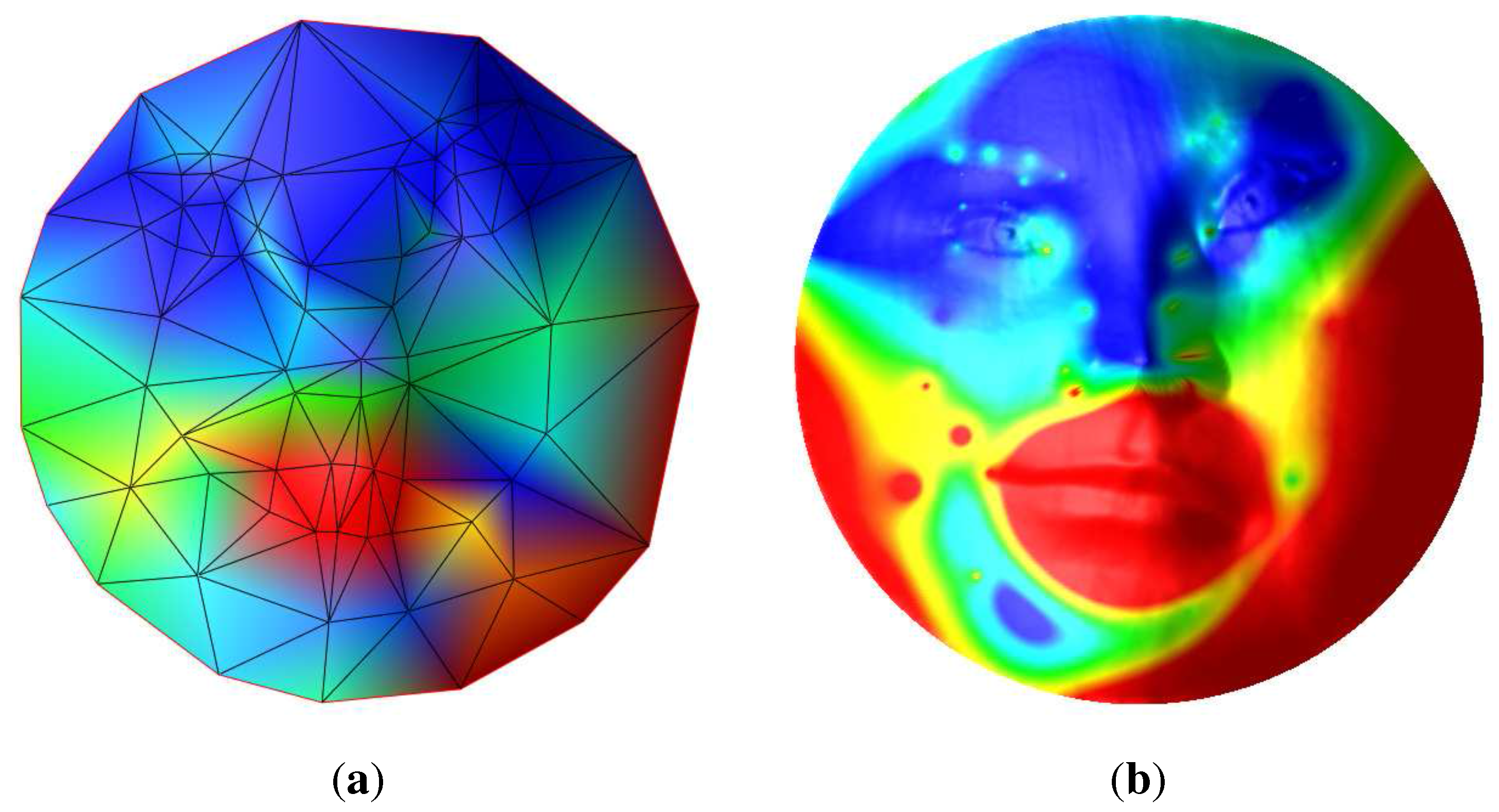
Under this framework, we use the following sparse-to-dense registration algorithm for 3D mesh surfaces with large deformations. It includes three stages: (1) feature extraction: we extract the feature points and their correspondence using the method of the Active Appearance Model (AAM) [40]; (2) Beltrami coefficients estimation: we construct the feature graph from the sparse feature points using Delaunay triangulation [41]; the matching between the sparse feature graphs induces the rough Beltrami differentials on the feature points. By smooth interpolation, such as harmonic map, the Beltrami differential function on the whole surface is estimated (see Figure 4). (3) Solving the Beltrami equation using discrete curvature flow: we compute the diffeomorphism between the dense mesh surfaces, which is uniquely determined by the Beltrami differential. The diffeomorphism gives the dense registration between surfaces. More computational details can be found in [27].

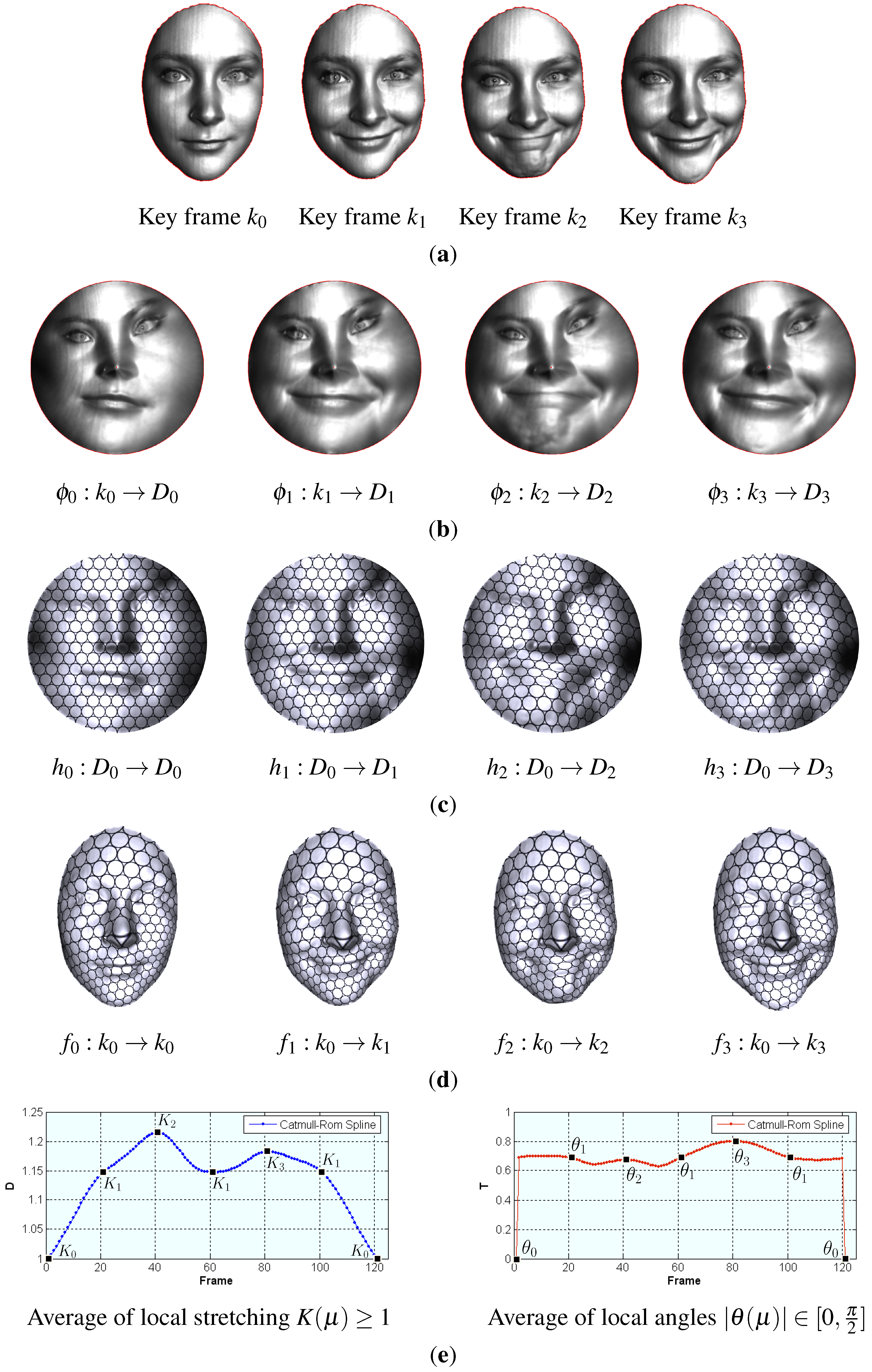
Figure 4 illustrates the Beltrami coefficients for the registration between key frames $k_0,k_2$ on the unit disk map (see Figure 5); the local stretching K is computed by Equation (2). Frame (a) visualizes the local stretching $K\left({\mu }_0\right)$ on the feature graph of key frame $k_0$; and (b) visualizes $K\left(\mu \right)$ on the dense mesh of $k_0$. The red color denotes the highest non-conformality and the blue color denotes the highest conformality. It can be easily seen that the muscles around the mouth have bigger non-conformal deformation; the bone structure on the forehead is rigid; therefore, the deformation is close to conformal. Figure 5a shows the four key frames $\{k_i,i=0..3\}$ from a 3D facial expression video; Figure 5b gives the corresponding conformal mappings to the unit disk; and Figure 5c,d show the registration results of $k_i$ to the reference frame $k_0$, where the one-to-one and onto registrations and the distortions are visualized by the consistent circle packing texture mappings, and the circles are changed to ellipses through the quasiconformal mapping associated with μ.

Figure 4. Quasiconformal diffeomorphic surface registration. (a) D on feature graph of $S_1$; (b) D on dense mesh ${\varphi }_1\left(S_1\right)$.

Figure 4. Quasiconformal diffeomorphic surface registration. (a) D on feature graph of $S_1$; (b) D on dense mesh ${\varphi }_1\left(S_1\right)$.

3.2. Generating Beltrami Differentials

Through the above approach, we generate a sequence of diffeomorphisms, $\{f_0,f_1,\dots ,f_n\}$, for a sequence of surfaces, $\{S_0,S_1,\dots ,S_n\}$. We usually use the first frame $S_0$ as the reference frame for generating diffeomorphisms, $f_k:S_0\to S_k$ for $k=0,\dots ,n$, as shown in Diagram (5).

$$\begin{array}{ccc}{S}_0& \stackrel{f_1}{\to }& S_1\\ S_0& \stackrel{f_2}{\to }& S_2\\ ⋮& \stackrel{\dots }{\to }& ⋮\\ S_0& \stackrel{f_n}{\to }& S_n\end{array}$$

(5)

As shown in Figure 5c,d, the diffeomorphisms between each key frame to frame $k_0$ are constructed by quasiconformal registrations, and their unique Beltrami differentials under a suitable normalization are computed accordingly. Here, the normalization is performed to map the nose tip of the facial surface to the origin of the unit disk and the middle point between two inner eye corners to the imaginary axis.

Essentially, given such a sequence of diffeomorphisms denoted as Beltrami coefficients and constructed from the same reference frame $S_0$, each interpolated Beltrami coefficient ${\mu }_t$ corresponds to a diffeomorphism $h_t$ in parameter space. By lifting the mapping from parameter space to the 3D surface, as shown in (4), the Beltrami coefficient ${\mu }_t$ is converted to a diffeomorphism $f_t$ from the reference frame $S_0$ to another surface frame $S_t$, which has the parameter domain $D_t$ associated with the ${\mu }_t$ from the reference parameter domain $D_0$ of $S_0$.

Figure 5. Diffeomorphism spline from the key frames of a 3D facial expression video. (a) Key frames; (b) conformal mappings to the unit disk; (c) consistent texture mappings on 2D conformal images; (d) consistent texture mappings on 3D original surfaces; (e) Catmull–Rom spline for diffeomorphisms of 7 key frames, $k_0,k_1,k_2,k_1,k_3,k_1,k_0$, from $k_0$.

Figure 5. Diffeomorphism spline from the key frames of a 3D facial expression video. (a) Key frames; (b) conformal mappings to the unit disk; (c) consistent texture mappings on 2D conformal images; (d) consistent texture mappings on 3D original surfaces; (e) Catmull–Rom spline for diffeomorphisms of 7 key frames, $k_0,k_1,k_2,k_1,k_3,k_1,k_0$, from $k_0$.

In the next step, we will use these diffeomorphisms with corresponding unique Beltrami differentials as the control points for constructing splines. The convex combination of Beltrami differentials is still a Beltrami differential. Therefore, the conventional spline scheme can be generalized to the Beltrami differential space, and consequently to the diffeomorphism space.

3.3. Constructing the Spline of Beltrami Differentials

In our framework, any type of spline (e.g., Bézier curve, Catmull–Rom spline) can be constructed on the given dataset of diffeomorphisms, which are represented by the Beltrami coefficients $\left\{{\mu }_k\right\}$. Catmull–Rom splines [42] are frequently used to get smooth interpolated motion between key frames, such as most camera path animations. They are popular mainly for being relatively easy to compute and guaranteeing that each key frame position will be hit exactly and that the tangents of the generated curve are continuous over multiple segments. In our applications, we use Catmull–Rom splines for smooth interpolation between the Beltrami differentials induced by key frame registrations.

Given $(n+1)$ points, ${\mu }_0,{\mu }_1,\dots ,{\mu }_n$, in the functional space, for each interval $(t_k,t_{k+1})$, the interpolation can be done with the following formula:

$$\mu \left(t\right)=h_{00}\left(t\right){\mu }_k+h_{10}{m}_k+h_{01}{\mu }_{k+1}+h_{11}{m}_{k+1}$$

(6)

where $h_{00},h_{10},h_{01},h_{11}$ are Hermite basis functions:

$$\begin{array}{cc}\hfill h_{00}\left(t\right)=(1+2t){(1-t)}^2& h_{10}\left(t\right)=t{(1-t)}^2\hfill \\ \hfill h_{01}\left(t\right)=t^2(3-2t)& h_{11}\left(t\right)=t^2(t-1)\hfill \end{array}$$

and $m_k$ is the tangent at $t_k$:

$$m_k=\frac{{\mu }_{k+1}-{\mu }_{k-1}}{t_{k+1}-t_{k-1}}$$

A dataset, $\{t_k,{\mu }_k\}$ for $k=0,\dots ,n$, can be interpolated by applying the above procedure on each interval, where the tangents are chosen in a sensible manner, meaning that the tangents for intervals sharing endpoints are equal. The interpolated curve then consists of piecewise cubic Hermite splines and is globally continuously differentiable in $(t_0,t_n)$.

In Figure 5e, we construct the Catmull–Rom spline for the Beltrami coefficients of the key frame diffeomorphisms, $\{{\mu }_i,i=0..3\}$, which is visualized by the average local stretching and the average local angle distortion of each interpolated diffeomorphism.

3.4. Quasiconformal Mapping for Diffeomorphism Recovery

The diffeomorphism $f:S_1\to S_2$ between surfaces can be recovered by the planar quasiconformal mapping $h:\mathbb{D}\to \mathbb{D}$, associated with a Beltrami differential, as shown in Diagram (4). The quasiconformal mapping can be computed by solving the Beltrami equation in Equation (1) and is unique up to a suitable normalization condition. Similarly, given a sequence of deformable surfaces and its diffeomorphism spline constructed, any interpolated diffeomorphism from the reference frame $S_1^0$ to $S_1^m$ at time $t_m\in [t_0,t_n]$ can be recovered from the corresponding Beltrami differential.

We apply the quasiconformal mapping algorithm based on the auxiliary metric induced by the Beltrami coefficient μ to recover the diffeomorphism (see Theorem 9; the proof can be found in [9,38]). Algorithm 1 shows the computation of the auxiliary metric on a discrete triangular mesh [39]. We then use discrete surface Ricci flow [43] to map the triangular mesh to the canonical domain, by using the auxiliary metric to replace the induced Euclidean metric of the original surface.

Algorithm 1 Auxiliary metric-based quasiconformal mapping.

Require:  A triangular mesh $M=(V,E,F)$ with conformal parameterization $z:V\to \mathbb{C}$ and discrete Beltrami differential $\mu :V\to \mathbb{C}$ defined on the conformal structure.

Ensure: Quasiconformal mapping $f:M\to \mathbb{D}$ satisfying the Beltrami equation with μ. Compute a conformal mapping $\varphi :M\to \mathbb{D}$ using discrete surface Ricci flow. for all edge $[v_i,v_j]\in M$ do  Compute the edge length $l_{ij}$ using the induced Euclidean metric.  Compute the derivative of conformal coordinates on $[v_i,v_j]$, $d{z}_{ij}\leftarrow \varphi \left(v_j\right)-\varphi \left(v_i\right)$.  Compute the Beltrami differential on $[v_i,v_j]$, ${\mu }_{ij}\leftarrow \frac{1}{2}(\mu \left(v_i\right)+\mu \left(v_j\right))$.  Compute the scalar of metric ${\lambda }_{ij}\leftarrow \frac{|d{z}_{ij}+{\mu }_{ij}d{\overline{z}}_{ij}|}{|d{z}_{ij}|}$.  Compute the auxiliary metric ${\tilde{l}}_{ij}\leftarrow {\lambda }_{ij}{l}_{ij}$. end for Compute the conformal mapping f using Ricci flow based on the auxiliary metric.

4. Experimental Results

We demonstrate the efficiency and efficacy of our method by constructing the diffeomorphism splines for both images and real scanned 3D surface sequences with large non-rigid deformations. The surfaces are represented as dense triangular meshes. In the following, we explain the experimental results on the construction of the diffeomorphism spline and the related applications.

4.1. Diffeomorphism Splines for Shape Modeling

The spline based on diffeomorphisms has much potential in shape modeling. Shape is manipulated in a general diffeomorphism space, which is essentially equal to a functional space of a special form. Any arbitrary shape is regarded as a diffeomorphism from a reference shape with the same topology. The spline provides the smooth and continuous interpolation path in this space. In this sense, the diffeomorphism space is general to handle any diffeomorphic deformations, subsuming the special categories of rigid motions, isometric transformations and conformal mappings. Any kind of physical and natural deformations, large or small, rigid or non-rigid, can be operated in the same way.

The diffeomorphism space also provides a way to compose diffeomorphisms. Suppose two diffeomorphisms, $f_1:S_1^0\to S_1,f_2:S_2^0\to S_2$. If the diffeomorphisms are from the same reference, then the composed diffeomorphism $f:S_1\to S_2$ is $f=f_2\circ f_1^{-1}$. If they are from different references, then for another diffeomorphism $f_0:S_1^0\to S_2^0$ between two references, the composition is $f=f_2\circ f_0^{-1}\circ f_1^{-1}$. This operation allows modeling diffeomorphisms in a back and forth way.

It is important to note that this work focuses on modeling the “diffeomorphisms” of surfaces in parameter space, not generating the “embeddings” of surfaces in 3D. This is also the difference from the diffeomorphisms obtained from statistical models [44]. The 3D geometry from the interpolated diffeomorphism of the parameter domain can be recovered based on the conformal representation theorem [37], which will be explored in future work.

Given the finite number of key diffeomorphic deformations of a reference shape, we can formulate each deformation as a diffeomorphism of the reference. Figure 5 gives the pipeline for computing the Catmull–Rom spline from key frames. This framework provides a practical and efficient tool for modeling shapes and accordingly has a broad range of applications. Here, we introduce several key applications in detail, such as 2D animation and inter-frame registration in 3D video.

4.2. Animation

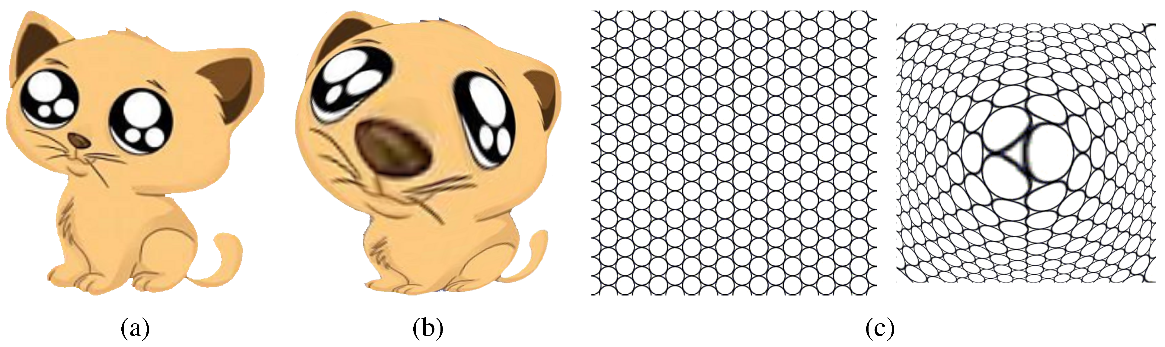
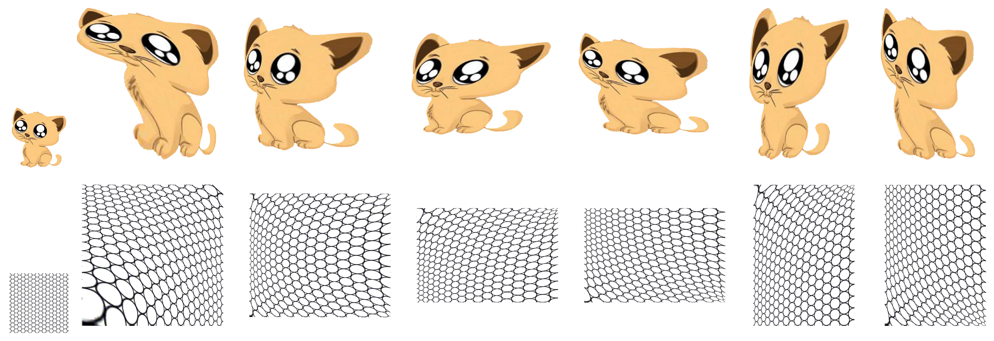
The spline for key diffeomorphisms generates the smooth animation path. The key diffeomorphisms can be learned from the given deformations (e.g., key frames in a video) based on the proposed surface registration method in this work. They also can be generated manually or computed analytically by designers. Figure 6 shows the diffeomorphisms of a regular square D (as shown in the left-most frame) to itself. Each diffeomorphism is a quasiconformal mapping of the regular square. The first row shows the deformation frames of the kitty image. The second row demonstrates the the quasiconformality of diffeomorphisms through the consistent circle-packing texture mapping results.

Figure 6. Animation with irregular deformations. The distortion of circles to ellipses visualizes the quasiconformality of diffeomorphisms.

Figure 6. Animation with irregular deformations. The distortion of circles to ellipses visualizes the quasiconformality of diffeomorphisms.

4.3. Inter-Frame Registration and Tracking

In the physical world, the deformation for a surface is generally diffeomorphic. A spatial-temporal sequence (video) of deformable non-rigid surfaces can be extracted as a sequence of diffeomorphisms of the reference surface. Key frames are frequently used for practical video editing purposes. In this work, the diffeomorphisms between frames are generated based on spline interpolation. This naturally induces the inter-frame registration within one video, even among videos.

We select the first key frame $k_0$ as the reference surface. Each key frame $k_i$ is a diffeomorphism $f_i$ of $k_0$. The diffeomorphism can be represented by a complex function, the Beltrami differential ${\mu }_i$. The Beltrami coefficients for key frames $k_0,k_1,\dots ,k_n$ are ${\mu }_0,{\mu }_1,\dots ,{\mu }_n$, respectively.

Figure 5 shows the diffeomorphism spline for key frames in a 3D video of a human face with expression changes.

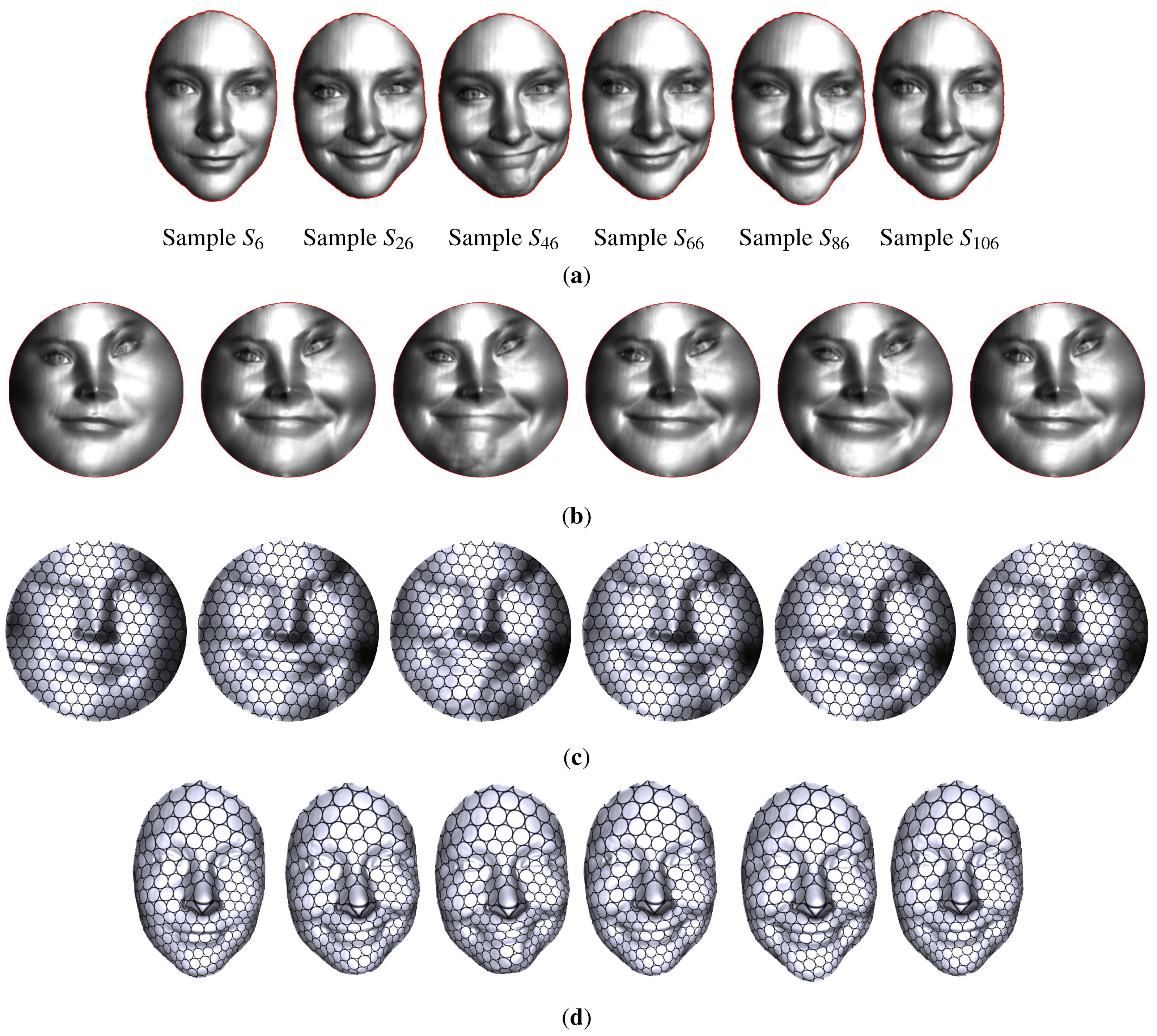
Figure 7. Diffeomorphisms interpolation and its application for inter-frame registration. (a) Surface samples $S_{t_i}$ corresponding to interpolated diffeomorphisms $f_{t_i}\left({\mu }_{t_i}\right)$; (b) corresponding interpolated diffeomorphisms on the 2D domain $h_{t_i}\left({\mu }_{t_i}\right)$; (c) Consistent texture mappings on interpolation frames $h_{t_i}:D_0\to D_{t_i}$; (d) consistent texture mappings on interpolation frames $f_{t_i}:k_0\to S_{t_i}$.

Figure 7. Diffeomorphisms interpolation and its application for inter-frame registration. (a) Surface samples $S_{t_i}$ corresponding to interpolated diffeomorphisms $f_{t_i}\left({\mu }_{t_i}\right)$; (b) corresponding interpolated diffeomorphisms on the 2D domain $h_{t_i}\left({\mu }_{t_i}\right)$; (c) Consistent texture mappings on interpolation frames $h_{t_i}:D_0\to D_{t_i}$; (d) consistent texture mappings on interpolation frames $f_{t_i}:k_0\to S_{t_i}$.

Four types of key frames are extracted $k_0,k_1,k_2,k_3$ in Figure 5a based on the conformal module signature as in [32], mainly describing the deformation intensity of the mouth area. The video is summarized as a sequence with seven key frames, $k_0,k_1,k_2,k_1,k_3,k_1,k_0$, where $k_1$ appears three times, because the expression change is repeated. Figure 5b shows their conformal maps on the unit disk. The diffeomorphic registrations between each key frame to the frame $k_0$ are constructed by quasiconformal mappings as stated in Section 3.1. The one-to-one correspondence is visualized by the consistent circle-packing texture mappings on both 2D conformal images Figure 5c and 3D original surfaces Figure 5d. The shape change of circles to ellipses demonstrates the quasiconformal deformations of expressions (Beltrami coefficients μ of the diffeomorphisms) from the reference. The diffeomorphism spline Figure 5e is then constructed using the key frame diffeomorphisms. Each interval of the spline has 19 samples, and each sample represents a diffeomorphism. Therefore, the whole spline has 121 samples $S_0,S_1,\dots ,S_{120}$, where $S_0=S_{120}=k_0,S_{20}=S_{60}=S_{100}=k_1,S_{40}=k_2,S_{80}=k_3$. The spline is illustrated by the statistics on the local stretching $K\left(\mu \right)$ and local angle $\theta \left(\mu \right)$, computed by (2) and (3), respectively. The diffeomorphisms are quasiconformal, except at the endpoints, which denote the identity map of the reference frame $k_0$ to itself.

The inter-frame registration is generated through the diffeomorphism spline interpolation as follows. In our current modeling, for a sample at $t_i$ of the diffeomorphism spline, we locate the corresponding 3D frame $S_{t_i}$ in the whole video with the same parameter $t_i$. By the interpolated Beltrami coefficient ${\mu }_{t_i}$ and the surface registration Diagram (4), the registration (diffeomorphism) between the reference key frame and the current interpolated frame $f_{t_i}:k_0\to S_{t_i}$ can be obtained directly. Figure 7a,b show the 2D/3D frames corresponding to the six interpolation samples ($t_i=6,26,46,66,86,106$) of the spline in Figure 5e. The consistent circle packing texture mappings in (c,d) visualize the inter-frame registration and deformation between 3D frame $S_{t_i}$ and $k_0$. The texture and normal information of the interpolated frames are interpolated accordingly through the one-to-one correspondence among the key frames.

4.4. Performance

We implement our algorithm using generic C++ on the Windows platform. The linear systems are solved using the conjugate gradient method. The experiments are carried out on a desktop with 3.40 GHZ CPU, 3.93 G RAM. The human face surfaces were captured using the phase shifting structured light method [10], which are discretely represented as triangular meshes. Each raw scan of human facial expression in Figure 5 has about $120k$ triangles. We use the raw data for generating the key frame registrations (diffeomorphisms). In generating diffeomorphism interpolations, we use a disk mesh with $25k$ vertices as the reference domain for 3D human faces and a regular square mesh with $10k$ vertices as the reference for image cases, which result in the consistent size of meshes and Beltrami coefficients. The computational time is reported in Table 1. The accuracy of inter-frame registration is measured by the averaged relative Hausdorff distance [24] between the source surface and the deformed result, which is close to 0.003. The registration can also be visually evaluated through the consistent texture mapping results on the original 3D surfaces. The experimental results show that the registration results are satisfactory.

In this work, we focus on topological disk surfaces. This proposed framework can handle any diffeomorphisms for general surfaces with more complicated topologies, such as the high genus cases. The only difference is that in the general manifold setting, the Beltrami coefficient is generalized to the Beltrami differential. Given a general surface, based on the uniformization theorem, a canonical domain associated with a specific rigid transformation group can be generated from the induced Euclidean metric. With that, the auxiliary metric method can be directly generalized to use the Beltrami differential [38,39] according to Theorem 9. This generalization will be explored in our future work.

Table 1. Computational time (seconds).

Model	Human Face Scan	Disk Reference Mesh	Square Reference Mesh
vertex#	$60k$	25,088	10,000
face#	$120k$	49,672	19,602
$T_c$	83	36	32
$T_b$	105	50	24
$T_s$	-	10	5
$T_q$	-	40	32

Note: $T_c$, conformal map for one frame; $T_b$, Beltrami differential computed by quasiconformal registration for one diffeomorphism; $T_s$, spline construction for 7 key frames with 19 samples in each interval; $T_q$, diffeomorphism recovery by quasiconformal map for one interpolation point.

Table 1. Computational time (seconds).

Model	Human Face Scan	Disk Reference Mesh	Square Reference Mesh
vertex#	$60k$	25,088	10,000
face#	$120k$	49,672	19,602
$T_c$	83	36	32
$T_b$	105	50	24
$T_s$	-	10	5
$T_q$	-	40	32

Note: $T_c$, conformal map for one frame; $T_b$, Beltrami differential computed by quasiconformal registration for one diffeomorphism; $T_s$, spline construction for 7 key frames with 19 samples in each interval; $T_q$, diffeomorphism recovery by quasiconformal map for one interpolation point.

5. Conclusions

In this work, we propose a novel spline scheme of modeling finite dimensional submanifolds in diffeomorphism space by generalizing conventional splines in three dimensional Euclidean space. Based on quasiconformal geometry, the diffeomorphism space has a one-to-one correspondence to the space of Beltrami differentials, and the convex combination of Beltrami differentials is still a Beltrami differential. Therefore, the conventional spline scheme can be generalized to the Beltrami differential space and, consequently, to the diffeomorphism space. Our experiments on 2D animation and inter-frame registration and tracking in 3D video demonstrate the efficiency and efficacy of diffeomorphism splines. The diffeomorphism spline scheme is general for any topological surfaces and has broad impacts on shape modeling and analysis problems and applications, which we will explore in our future works.

References

- Piegl, L.; Tiller, W. The NURBS Book; Springer: Berlin, Germany, 1997. [Google Scholar]
- Farin, G. Curves and Surfaces for Computer Aided Geometric Design: A Practical Guide; Academic Press: San Diego, CA, USA, 1990. [Google Scholar]
- Farin, G.; Hansford, D. The Essentials of CAGD; A K Peters, Ltd.: Natic, MA, USA, 1990. [Google Scholar]
- Yang, Y.; Zeng, W. Optimizing Equiareality of NURBS Surfaces using Composite Mobius Transformations. J. Comput. Appl. Math. 2015, 279, 1–12. [Google Scholar] [CrossRef]
- Yang, Y.; Zeng, W. Equiareal parameterizations of nurbs surfaces. Graph. Models 2014, 76, 43–55. [Google Scholar] [CrossRef]
- Yang, Y.; Zeng, W.; Yang, C.; Deng, B.; Meng, X.; lyengar, S. An algorithm to improve parameterizations of rational Bézier surfaces using rational bilinear reparameterization. Comput. Aided Des. 2013, 45, 628–638. [Google Scholar] [CrossRef]
- Yang, Y.; Zeng, W.; Yang, C.; Meng, X.; Yong, J.; Deng, B. G1 continuous approximate curves on NURBS surfaces. Comput. Aided Des. 2012, 44, 824–834. [Google Scholar] [CrossRef]
- Ramamoorthi, R.; Barr, A.H. Fast construction of accurate quaternion splines. In Proceedings of the 24th Annual Conference on Computer Graphics and Interactive Techniques, 1997, SIGGRAPH ’97, Los Angeles, CA, USA, 3–8 August 1997; pp. 287–292.
- Ahlfors, L. Lectures in Quasiconformal Mappings; Van Nostrand Reinhold: New York, NY, USA, 1966. [Google Scholar]
- Wang, Y.; Gupta, M.; Zhang, S.; Wang, S.; Gu, X.; Samaras, D.; Huang, P. High Resolution Tracking of Non-Rigid Motion of Densely Sampled 3D Data Using Harmonic Maps. IJCV 2008, 76, 283–300. [Google Scholar] [CrossRef]
- Vemuri, B.; Mitiche, A.; Aggarwal, J. Curvature-based Representation of Objects from Range Data. Image Vison Comput. 1986, 4, 107–114. [Google Scholar] [CrossRef]
- Ruiz-Correa, S.; Shapiro, L.; Meila, M. A New Paradigm for Recognizing 3D Object Shapes from Range Data. In Proceedings of the ICCV, Nice, France, 13–16 October 2003; pp. 1126–1133.
- Sun, Y.; Abidi, M. Surface Matching by 3D Point’s Fingerprint. In Proceedings of the ICCV, Vancouver, Canada, 7–14 July 2001; Volume II, pp. 263–269.
- Frome, A.; Huber, D.; Kolluri, R.; Bulow, T.; Malik, J. Recognizing Objects in Range Data Using Regional Point Descriptors. In Proceedings of the ECCV, Prague 1, Czech Republic, 11–14 May 2004; Volume III, pp. 224–237.
- Funkhouser, T.; Min, P.; Kazhdan, M.; Chen, J.; Halderman, A.; Dobkin, D.; Jacobs, D. A Search Engine for 3D Models. ACM TOG 2003, 22, 83–105. [Google Scholar] [CrossRef]
- Osada, R.; Funkhouser, T.; Chazelle, B.; Dobkin, D. Shape Distributions. ACM TOG 2002, 21, 807–832. [Google Scholar] [CrossRef]
- Terzopoulos, D.; Witkin, A.; Kass, M. Constraints on Deformable Models: Recovering 3D Shape and Nonrigid Motion. Artif. Intell. 1988, 35, 91–123. [Google Scholar] [CrossRef]
- Huang, X.; Paragios, N.; Metaxas, D. Establishing Local Correspondences towards Compact Representations of Anatomical Structures. In Proceedings of the MICCAI, Montréal, Canada, 15–18 November 2003; pp. 926–934.
- Malladi, R.; Sethian, J.A.; Vemuri, B.C. A Fast Level Set based Algorithm for Topology-Independent Shape Modeling. J. Math. Imaging Vision 1996, 6, 269–290. [Google Scholar] [CrossRef]
- Sharon, E.; Mumford, D. 2D-Shape Analysis Using Conformal Mapping. IJCV 2006, 70, 55–75. [Google Scholar] [CrossRef]
- Feiszli, M.; Mumford, D. Shape Representation via Conformal Mapping. In Proceedings of the SPIE 6498, Computational Imaging V, San Jose, CA, USA, 7 February 2007.
- Lipman, Y. Conformal Wasserstein Distances: Comparing Surfaces in Polynomial Time. arXiv:1103.4408. 2011. [Google Scholar]
- Bronstein, A.M.; Bronstein, M.M.; Kimmel, R. Generalized Multidimensional Scaling: A Framework for Isometry-invariant Partial Surface Matching. Proc. Natl. Acad. Sci. USA 2006, 103, 1168–1172. [Google Scholar] [CrossRef] [PubMed]
- Zeng, W.; Samaras, D.; Gu, X.D. Ricci Flow for 3D Shape Analysis. IEEE TPAMI 2010, 32, 662–677. [Google Scholar] [CrossRef] [PubMed]
- Zeng, Y.; Wang, C.; Wang, Y.; Gu, X.; Samaras, D.; Paragios, N. Dense Non-rigid Surface Registration Using High-Order Graph Matching. In Proceedings of the IEEE CVPR, San Francisco, NC, USA, 13–18 June 2010.
- Lui, L.M.; Wong, T.W.; Zeng, W.; Gu, X.; Thompson, P.M.; Chan, T.F.; Yau, S.T. Optimization of Surface Registrations Using Beltrami Holomorphic Flow. J. Sci. Comput. 2012, 50, 557–585. [Google Scholar] [CrossRef]
- Zeng, W.; Gu, X. Registration for 3D Surfaces with Large Deformations Using Quasi-Conformal Curvature Flow. In Proceedings of the CVPR, Colorado Springs, CO, USA, 20–25 June 2011; pp. 2457–2464.
- Lui, L.M.; Wong, T.W.; Thompson, P.M.; Chan, T.F.; Gu, X.; Yau, S.T. Compression of Surface Registrations Using Beltrami Coefficient. In Proceedings of the IEEE CVPR, San Francisco, NC, USA, 13–18 June 2010.
- Wong, T.W.; Gu, X.; Chan, T.F.; Lui, L.M. Parallelizable Inpainting and Refinement of Diffeomorphisms Using Beltrami Holomorphic Flow. In Proceedings of the ICCV, Barcelona, Spain, 6–13 November 2011.
- Lipman, Y.; Kim, V.G.; Funkhouser, T.A. Simple formulas for quasiconformal plane deformations. ACM TOG 2012, 31. [Google Scholar] [CrossRef]
- Weber, O.; Myles, A.; Zorin, D. Computing Extremal Quasiconformal Maps. Comput. Graph. Forum 2012, 31, 1679–1689. [Google Scholar] [CrossRef]
- Zeng, W.; Gu, X. 3D Dynamics Analysis in Teichmüller Space. In Proceedings of the ICCV Workshop on Dynamic Shape Capture and Analysis Recognition (4DMOD’11), Barcelona, Spain, 13 November 2011.
- Henrici, P. Applied and Computational Complex Analysis; Volume 3; Wiley-Intersecience: New York, NY, USA, 1988. [Google Scholar]
- Farkas, H.M.; Kra, I. Riemann Surfaces; Springer: Berlin, Germany, 2004. [Google Scholar]
- Chow, B. The Ricci Flow on the 2-sphere. J. Differ. Geom. 1991, 33, 325–334. [Google Scholar]
- Hamilton, R.S. The Ricci Flow on Surfaces. Math. Gen. Relativ. 1988, 71, 237–262. [Google Scholar]
- Gu, D.X.; Zeng, W.; Luo, F.; Yau, S.T. Numerical Computation of Surface Conformal Mappings. Comput. Methods Funct. Theory 2011, 11, 747–787. [Google Scholar] [CrossRef]
- Zeng, W.; Lui, L.M.; Luo, F.; Chan, T.; Yau, S.T.; Gu, X. Computing Quasiconformal Maps Using an Auxiliary Metric with Discrete Curvature Flow. Numer. Math. 2012, 121, 671–703. [Google Scholar] [CrossRef]
- Zeng, W.; Luo, F.; Yau, S.T.; Gu, X. Surface Quasi-Conformal Mapping by Solving Beltrami Equations. In Proceedings of the IMA International Conference on Mathematics of Surfaces XIII, York, UK, 7–9 September 2009; pp. 391–408.
- Cootes, T.F.; Edwards, G.J.; Taylor, C.J. Active Appearance Models. IEEE TPAMI 2001, 23, 681–685. [Google Scholar] [CrossRef]
- Shewchuk, J.R. Triangle: Engineering a 2D Quality Mesh Generator and Delaunay Triangulator. Appl. Comput. Geom. Towards Geom. Eng. 1996, 1148, 203–222. [Google Scholar]
- Catmull, E.; Rom, R. A class of local interpolating splines. Comput. Aided Geom. Des. 1974, 74, 317–326. [Google Scholar]
- Jin, M.; Kim, J.; Luo, F.; Gu, X. Discrete Surface Ricci Flow. IEEE TVCG 2008, 14, 1030–1043. [Google Scholar] [CrossRef] [PubMed]
- Taylor, C.; Twining, C.; Davies, R. Statistical Models of Shape—Optimisation and Evaluation; Springer: Berlin, Germany, 2008. [Google Scholar]
© 2015 by the authors; licensee MDPI, Basel, Switzerland. This article is an open access article distributed under the terms and conditions of the Creative Commons Attribution license (http://creativecommons.org/licenses/by/4.0/).
Share and Cite
MDPI and ACS Style
Zeng, W.; Razib, M.; Shahid, A.B. Diffeomorphism Spline. Axioms 2015, 4, 156-176. https://doi.org/10.3390/axioms4020156
AMA Style
Zeng W, Razib M, Shahid AB. Diffeomorphism Spline. Axioms. 2015; 4(2):156-176. https://doi.org/10.3390/axioms4020156
Chicago/Turabian StyleZeng, Wei, Muhammad Razib, and Abdur Bin Shahid. 2015. "Diffeomorphism Spline" Axioms 4, no. 2: 156-176. https://doi.org/10.3390/axioms4020156