R-Matrices, Yetter-Drinfel'd Modules and Yang-Baxter Equation

Institut de Mathématiques de Jussieu–Paris Rive Gauche, UMR7586, Bâtiment Sophie Germain, Case 7012, 75205 PARIS Cedex 13, France
Axioms 2013, 2(3), 443-476; https://doi.org/10.3390/axioms2030443
Submission received: 14 August 2013
/
Revised: 28 August 2013
/
Accepted: 30 August 2013
/
Published: 5 September 2013
(This article belongs to the Special Issue Hopf Algebras, Quantum Groups and Yang-Baxter Equations 2013)
Abstract
:In the first part we recall two famous sources of solutions to the Yang-Baxter equation—R-matrices and Yetter-Drinfel′d (=YD) modules—and an interpretation of the former as a particular case of the latter. We show that this result holds true in the more general case of weak R-matrices, introduced here. In the second part we continue exploring the “braided” aspects of YD module structure, exhibiting a braided system encoding all the axioms from the definition of YD modules. The functoriality and several generalizations of this construction are studied using the original machinery of YD systems. As consequences, we get a conceptual interpretation of the tensor product structures for YD modules, and a generalization of the deformation cohomology of YD modules. This homology theory is thus included into the unifying framework of braided homologies, which contains among others Hochschild, Chevalley-Eilenberg, Gerstenhaber-Schack and quandle homologies.
1. Introduction
The Yang-Baxter equation (YBE) is omnipresent in modern mathematics. Its realm stretches from statistical mechanics to quantum field theory, covering quantum group theory, low-dimensional topology and many other fascinating areas of mathematics and physics. The attemps to understand and classify all solutions to the Yang-Baxter equation (often referred to as braidings, since they provide representations of braid groups) have been fruitless so far. Nevertheless we dispose of several methods of producing vast families of such solutions, often endowed with an extremely rich structure.
In Section 2 we review two major algebraic sources of braidings, which have been thouroughly studied from various viewpoints over the past few decades. The first one is given by R-matrices for quasi-triangular bialgebras, dating back to V.G. Drinfel′d’s celebrated 1986 ICM talk [1]. The second one comes from Yetter-Drinfel′d modules (=YD modules) over a bialgebra, introduced by D. Yetter in 1990 under the name of “crossed bimodules” (see [2]) and rediscovered later by different authors under different names (see for instance the paper [3] of S.L. Woronowicz, where he implicitely considers a Hopf algebra as a YD module over itself). All these notions and constructions are recalled in detail in Section 2.2 and Section 2.3.
Note that we are interested here in not necessarily invertible braidings; that is why most constructions are effectuated over bialgebras rather than Hopf algebras, though the latter are more current in literature. Section 3.2 contains an example where the non-invertibility does matter.
It was shown in S. Montgomery’s celebrated book ([4], 10.6.14) that R-matrix solutions to the YBE can be interpreted as particular cases of Yetter-Drinfel′d type solutions. We recall this result and its categorical version (due to M. Takeuchi, cf. [5]) in Section 2.4. Our original contribution consists in a generalization of this result: we introduce the notion of weak R-matrix for a bialgebra H and show it to be sufficient for endowing any H-module with a YD module structure over H (cf. the charts on p. 456).
In Section 3 we explore deeper connections between YD modules (and thus R-matrices, as explained above) and the YBE. We show that YD modules give rise not only to braidings, but also to higher-level braided structures, called braided systems. Here we briefly explain this concept after a short recapitulation of two category-theoretic viewpoints on the YBE—a “local” and a “global” ones.
The first one is rather straightforward: in a strict monoidal category one looks for objects V and endomorphisms σ of satisfying (YBE). Such V’s are called braided objects in A more categorical approach consists in working in a “globally” braided monoidal category, as defined in 1993 by A. Joyal and R.H. Street ([6]). Concretely, a braiding on a monoidal category is a natural family of morphisms compatible with the monoidal structure, in the sense of Equations (2) and (3). Every object V of such a category is braided, via See [5] for a comparison of “local” and “global” approaches, in particular in the the context of the definition of braided Hopf algebras. Well-known braidings on the category of modules over a quasi-triangular bialgebra and in that of YD modules over a bialgebra are recalled in Section 2.2 and Section 2.3.
Now, the notion of braided system in is a multi-term version of that of braided object: it is a family of objects in endowed with morphisms for all satisfying a system of mixed YBEs. This notion was defined and studied in [7] (see also [8]). The case appeared, under the name of Yang-Baxter system (or WXZ system), in the work of L. Hlavatý and L. Šnobl ([9]). See Section 3.1 for details.
In Section 3.2, we present a braided system structure on the family for a YD module M over a finite-dimensional -bialgebra H (here is a field, and is the linear dual of H). Note that several ’s from this system are highly non-invertible. Its subsystem is the braided system encoding the bialgebra structure, constructed and explored in [8], and related to, but different from, the braided system considered by F.F. Nichita in [10] (see also [11]).
In order to treat the above construction in a conceptual way and extend it to a braided system structure on for YD modules over we introduce the concept of Yetter-Drinfel′d system and show it to be automaticaly endowed with a braiding. See Section 3.3 for details, and Section 3.4 for examples.
In Section 3.5 we show the functoriality and the precision of the above braided system construction. The functoriality is proved by exhibiting the category inclusion (41). Precision means that the described braided system structure on captures all the algebraic information about the YD module in the sense that each mixed YBE for this system is equivalent to an axiom from the definition of a YD module, and each YD axiom gets a “braided” interpretation in this way.
Section 3.6 contains an unexpected application of the braided system machinery. Namely, it allows us to recover the two tensor product structures for YD modules, proposed by L.A. Lambe and D.E. Radford in [12], from a conceptual viewpoint.
Applying the general braided (co)homology theory from [8,13] (recalled in Section 3.7) to the braided systems above, we obtain in Section 3.8 a rich (co)homology theory for (families of) YD modules. It contains in particular the deformation cohomology of YD modules, introduced by F. Panaite and D. Ştefan in [14]. The results of Section 2.4 give then for free a braided system structure for any module over a finite-dimensional quasi-triangular -bialgebra with a corresponding (co)homology theory. Besides a generalization of the Panaite-Ştefan construction, our “braided” tools allow to considerably simplify otherwise technical verifications from their theory. Moreover, our approach allows to consider YD module (co)homologies in the same unifying framework as the (co)homologies of other algebraic structures admitting a braided interpretation, e.g., associative and Leibniz (or Lie) algebras, self-distributive structures, bialgebras and Hopf (bi)modules (see [8,13]).
The paper is intended to be as elementary and self-contained as possible. Even widely known notions are recalled for the reader’s convenience. The already classical graphical calculus is extensively used in this paper, with
- ➛
- dots standing for vector spaces (or objects in a monoidal category),
- ➛
- horizontal gluing corresponding to the tensor product,
- ➛
- graph diagrams representing morphisms from the vector space (or object) which corresponds to the lower dots to that corresponding to the upper dots,
- ➛
- vertical gluing standing for morphism composition, and vertical strands for identities.
Note that all diagrams in this paper are to be read from bottom to top.
Throughout this paper we work in a strict monoidal category (Definition 2.1); as an example, one can have in mind the category of -vector spaces and -linear maps, endowed with the usual tensor product over
For an object V in and a morphism the following notation is repeatedly used:
2. Two Sources of Braidings Revisited
2.1. Basic Definitions
Definition 2.1 A strict monoidal (or tensor) category is a category endowed with
- ➛
- a tensor product bifunctor satisfying the associativity condition;
- ➛
- a unit object which is a left and right identity for
We work only with strict monoidal categories here for the sake of simplicity; according to a theorem of S. MacLane ([15]), any monoidal category is monoidally equivalent to a strict one. This justifies in particular parentheses-free notations like or The word “strict” is omitted but always implied in what follows.
The “local” categorical notion of braiding will be extensively used in this paper:
Definition 2.2. An object V in a monoidal category is called braided if it is endowed with a “local” braiding, i.e., a morphism
satisfying the (categorical) Yang-Baxter equation (=YBE)
Following D. Yetter ([2]), one should use the term pre-braiding here in order to stress that non-invertible σ’s are allowed; we keep the term braiding for simplicity.
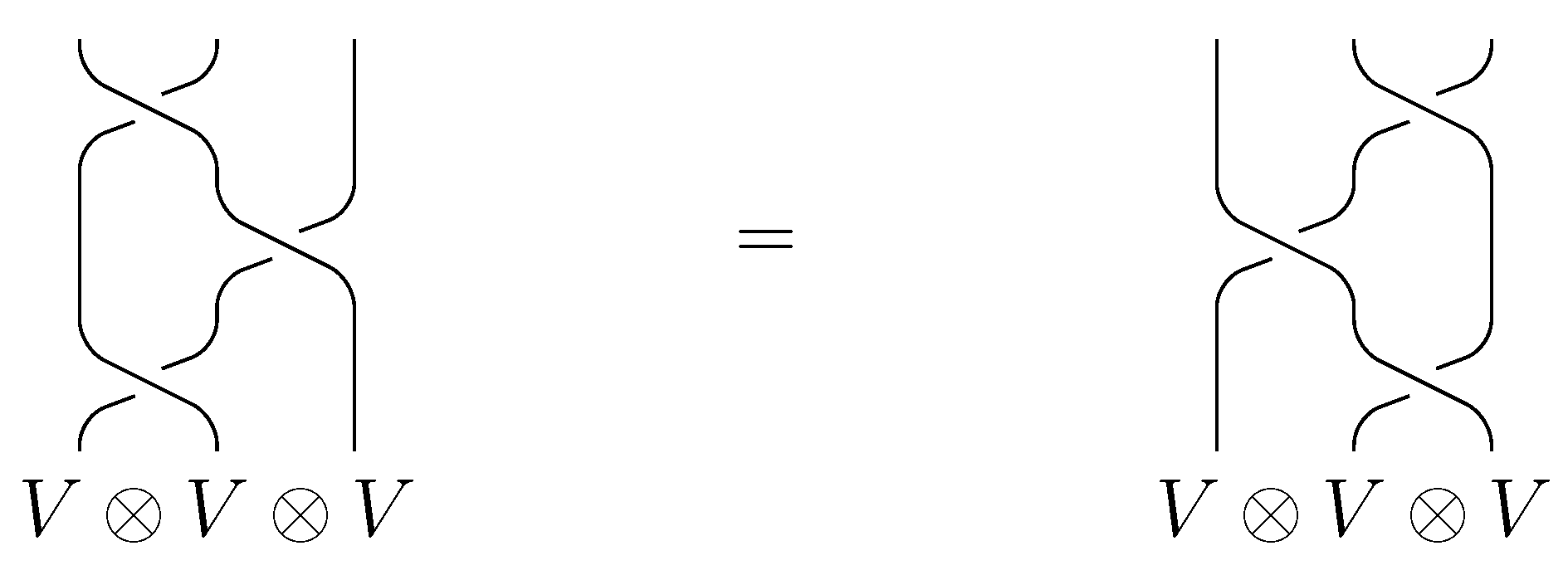
Graphically, the braiding is presented as ![Axioms 02 00443 i002]() . The diagrammatical counterpart of (YBE), depicted on Figure 1, is then the third Reidemeister move, which is at the heart of knot theory.
. The diagrammatical counterpart of (YBE), depicted on Figure 1, is then the third Reidemeister move, which is at the heart of knot theory.
 . The diagrammatical counterpart of (YBE), depicted on Figure 1, is then the third Reidemeister move, which is at the heart of knot theory.
 Figure 1.
Yang-Baxter equation ↔ Reidemeister move III.
The “global” categorical notion of braiding will also be used here, both for describing the underlying category and for constructing and systematizing new braidings:
Definition 2.3.
- ➛
- A monoidal category is called braided if it is endowed with a braiding (or a commutativity constraint), i.e., a natural family of morphisms indexed by objects of satisfyingfor any triple of objects “Natural” means herefor all objects and all morphisms
- ➛
- A braided category is called symmetric if its braiding is symmetric:
The part “monoidal” of the usual terms “braided monoidal” and “symmetric monoidal” are omitted in what follows.
Lemma 2.4. Every object V in a braided category is braided, with
Proof. Take and in the condition Equation (5) expressing naturality; this gives the YBE. ☐
We further define the structures of algebra, coalgebra, bialgebra and Hopf algebra in a monoidal category :
Definition 2.5.
- ➛
- A unital associative algebra (= UAA) in is an object A together with morphisms and satisfying the associativity and the unit conditions:A UAA morphism φ between UAAs and is a respecting the UAA structures:
- ➛
- A UAA in is called braided if it is endowed with a braiding σ compatible with the UAA structure. Using notation (1), this can be written as
- ➛
- A counital coassociative coalgebra (= coUAA) in is an object C together with morphisms and satisfying the coassociativity and the counit conditions:A coUAA morphism φ between coUAAs is a morphism in respecting the coUAA structures.
- ➛
- A coUAA in is called braided if it is endowed with a braiding σ compatible with the coUAA structure, in the sense analogous to Equations (8)–(11).
- ➛
- A left module over a UAA in is an object M together with a morphism respecting μ and ν:An A-module morphism φ between A-modules and is a respecting the A-module structures:The category of A-modules in and their morphisms is denoted byRight modules, left/right comodules over coUAAs and their morphisms are defined similarly.
- ➛
- A bialgebra in a braided category is a UAA structure and a coUAA structure on an object compatible in the following sense:A bialgebra morphism is a morphism which respects UAA and coUAA structures simultaneously.
- ➛
- If moreover H has an antipode, i.e., a morphism satisfyingthen it is called a Hopf algebra in
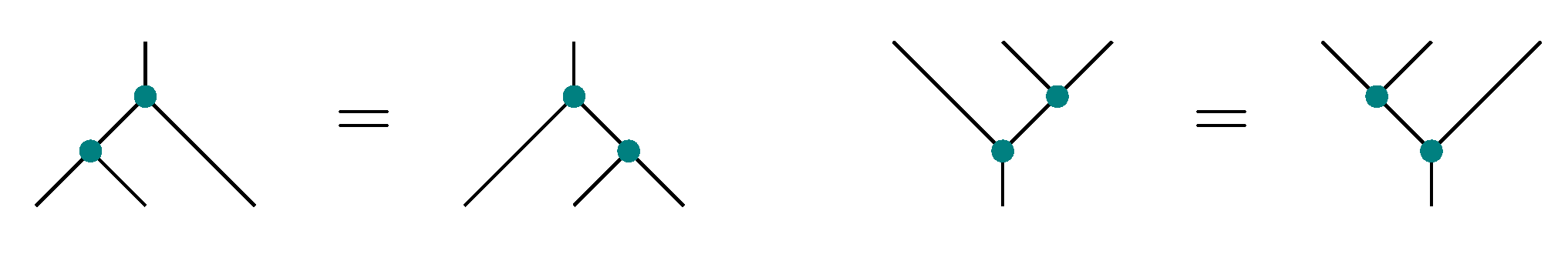
The notions of (braided) algebra and coalgebra, and of module and comodule, are mutually dual, while that of braiding, of bialgebra and Hopf algebra are self-dual; see [7,15] for more details on the categorical duality. Graphically, applying this duality consists simply in turning all the diagrams upside down, i.e., taking a horizontal mirror image. For instance, Figure 2 contains the graphical depictions of the associativity and the coassociativity axioms. Here and afterwards a multiplication μ is represented as ![Axioms 02 00443 i003]() , and a comultiplication Δ – as
, and a comultiplication Δ – as ![Axioms 02 00443 i004]() .
.
 , and a comultiplication Δ – as
  .
. Figure 2.
Associativity and coassociativity.

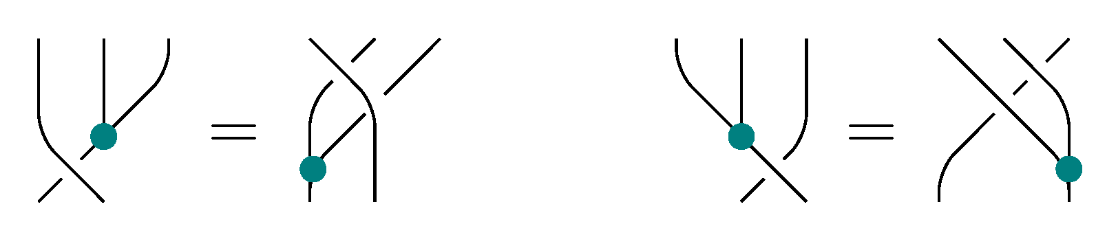
Graphical versions of several other axioms from the above definition are presented on Figure 3 and Figure 4.
Figure 3.
Compatibility conditions for a braiding and a comultiplication.

Figure 4.
Main bialgebra axiom (15).

Note that (15) is the only bialgebra axiom requiring a braiding on the underlying category
2.2. R-Matrices
From now on we work in a symmetric category Fix a bialgebra H in A bialgebra structure on H is precisely what is needed for the category of its left modules to be monoidal: the tensor product of H-modules and is endowed with the H-module structure
and the unit object is endowed with the H-module structure
In what follows we always assume this monoidal structure on
If one wants the category to be braided (and thus to provide solutions to the Yang-Baxter equation), an additional quasi-triangular structure should be imposed on The growing interest in quasi-triangular structures can thus be partially explained by their capacity to produce highly non-trivial solutions to the YBE. The most famous example is given by quantum groups (see for instance [16]), which will not be discussed here.
Definition 2.6. A bialgebra H in is called quasi-triangular if it is endowed with an R-matrix, i.e., a morphism satisfying the following conditions:
is the standard multiplication on the tensor product of two UAAs, and
are the twisted multiplication and comultiplication respectively.
The R-matrix R is called invertible if there exists a morphism such that
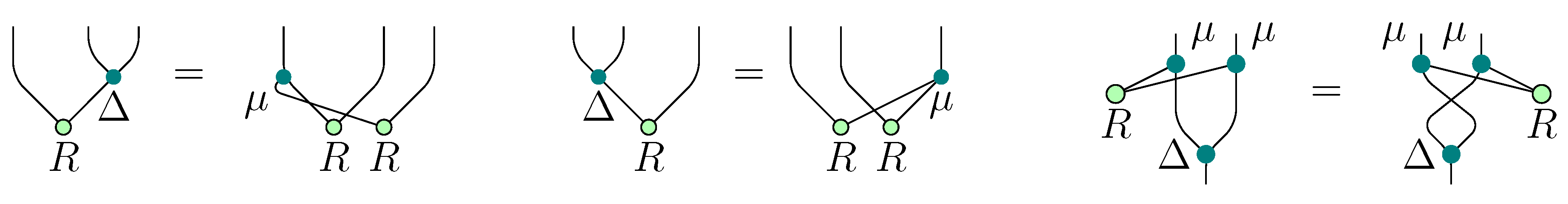
Figure 5 shows a graphical version of the conditions from the definition.
Figure 5.
Axioms for an R-matrix.
A well-known result affirms that a quasi-triangular bialgebra structure on H is precisely what is needed for its module category to be braided:
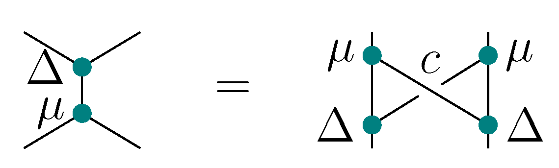
Theorem 1. The category of left modules over a quasi-triangular bialgebra H in can be endowed with the following braiding (cf. Figure 6):
Here R is the R-matrix of and c is the underlying symmetric braiding of the category
If the R-matrix is moreover invertible, then the braiding is invertible as well, with
Figure 6.
A braiding for H-modules.

All the statements of the theorem can be verified directly (see [16] or any other book on quantum groups). In Section 2.4 we will see an indirect proof based on a Yetter-Drinfel′d module interpretation of modules over a quasi-triangular bialgebra.
If one is only interested in solutions to the YBE, the following corollary of the above theorem is sufficient:
Corollary 2.7. Given a quasi-triangular bialgebra in any left module M over H is a braided object in with the braiding This braiding is invertible if the R-matrix R is.
Proof. Apply Lemma 2.4 to the braided category structure from Theorem 1. ☐
2.3. Yetter-Drinfel′d Modules
Yetter-Drinfel′d modules are known to be at the origin of a very vast family of solutions to the Yang-Baxter equation. According to [17,18,19], this family is complete if one restricts oneself to finite-dimensional solutions over a field This led L.A. Lambe and D.E. Radford to use the eloquent term quantum Yang-Baxter module instead of the more historical term Yetter-Drinfel′d module, cf. [12]. We recall here the definition of this structure and its most important properties.
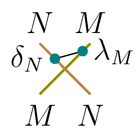
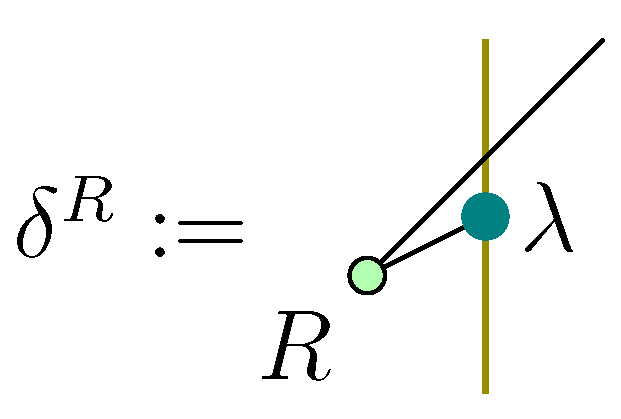
Definition 2.8. A Yetter-Drinfel′d (= YD) module structure over a bialgebra H in a symmetric category consists of a left H-module structure λ and a right H-comodule structure δ on an object satisfying the Yetter-Drinfel′d compatibility condition (cf. Figure 7)
The category of YD modules over a bialgebra H (with, as morphisms, those which are simultaneously H-module and H-comodule morphisms) is denoted by
Figure 7.
Yetter-Drinfel0d compatibility condition.

The name left-right Yetter-Drinfel′d module is more appropriate for the structure described in the definition; we shorten it for simplicity. One can also define right-left and (in the case when H is a Hopf algebra) right-right and left-left YD modules. If the antipode s of H is invertible, then all these notions are equivalent due to the notable correspondence between left and right H-module structures (similarly for comodules). For example, a right action can be transformed to a left one via

Example 2.9. A simple but sufficiently insightful example is given by the group algebra of a finite group which is a Hopf algebra via the linearization of the maps and for all For such an the notion of left H-module (in the category ) is easily seen to reduce to that of a -linear representation of and the notion of right H-comodule to that of a G-graded vector space with
The compatibility condition (YD) reads in this setting
(here the left H-action on M is denoted by a dot). In particular, H becomes a YD module over itself when endowed with the G-grading and the adjoint G-action
The category can be endowed with a monoidal structure in several ways (cf. [12]). We choose here the structure which makes the forgetful functor
monoidal, where is endowed with the monoidal structure described in Section 2.2. Concretely, the tensor product of YD modules and is endowed with the H-module structure (16) and the H-comodule structure
and the unit object is endowed with the H-modules structure (17) and the H-comodule structure
Note that using the twisted multiplication in the definition of is essential for assuring its YD compatibility with
The monoidal category defined this way possesses a famous braided structure:
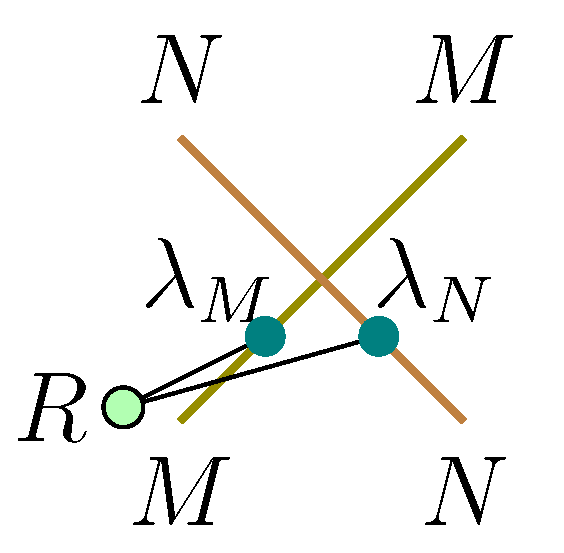
Theorem 2. The category of left-right Yetter-Drinfel′d modules can be endowed with the following braiding (cf. Figure 8):
If H is moreover a Hopf algebra with the antipode then the braiding is invertible, with
Figure 8.
A braiding for left-right YD modules.
The theorem can be proved by an easy direct verification.
Remark 2.10 The category can be endowed with a monoidal structure alternative to Equations (16) and (22). Namely, one can endow the tensor product of YD modules M and N with the “twisted” module and usual comodule structure:
Theorem 2 remains true in this setting if one replaces the braiding with its alternative version
This construction is best explained graphically. First, observe that the notions of bialgebra, YD module and braiding are stable by the central symmetry. In other words, the sets of diagrams representing the axioms defining these notions are stable by an angle π rotation (hence the notations etc. evoking rotation). Now, an angle π rotation of the H-module structure (16) is the H-comodule structure (27), and similarly for Equations (22) and (26). To conclude, note that the braiding is precisely an angle π rotation of (cf. Figure 8 and Figure 9). This alternative structure will be used in Section 3.
Figure 9.
An alternative braiding for left-right YD modules.

If one is only interested in solutions to the YBE, the following corollary is sufficient:
Corollary 2.11. Given a bialgebra H in any left-right YD module M over H is a braided object in with the braiding This braiding is invertible if H is moreover a Hopf algebra.
Proof. Apply Lemma 2.4 to the braided category structure from Theorem 2. ☐
Example 2.12. Applied to Example 2.9, the corollary gives an invertible braiding
for One recognizes (the linearization of) a familiar braiding for groups, which can alternatively be obtained using the machinery of self-distributive structures.
2.4. A Category Inclusion
The braided categories constructed in the two previous sections exhibit apparent similarities. We explain them here by interpreting the category of left modules over a quasi-triangular bialgebra H in a symmetric category as a full braided subcategory of the category of left-right Yetter-Drinfel′d modules over We further introduce a weaker notion of R-matrix for which the above category inclusion still holds true, in general without respecting the monoidal structures. In particular, if one is interested only in constructing solutions to the Yang-Baxter equation (cf. Corollaries 2.7 and 2.11), this weaker notion suffices.
Let and be a UAA and, respectively, a coUAA structures on an object H of A preliminary remark is first due.
Remark 2.13. The definition of Yetter-Drinfel′d module actually requires (not necessarily compatible) UAA and coUAA structures on H only. The category is no longer monoidal in this setting. However, a direct verification shows that Corollary 2.11 still holds true (the argument closely repeats that from the proof of Theorem 5 , point 2).
We thus do not suppose H to be a bialgebra unless explicitely specified.
Figure 10.
Module + R-matrix ⟼ comodule.

Now try to determine conditions on R which make a left-right Yetter-Drinfel′d module for any One arrives to the following set of axioms:
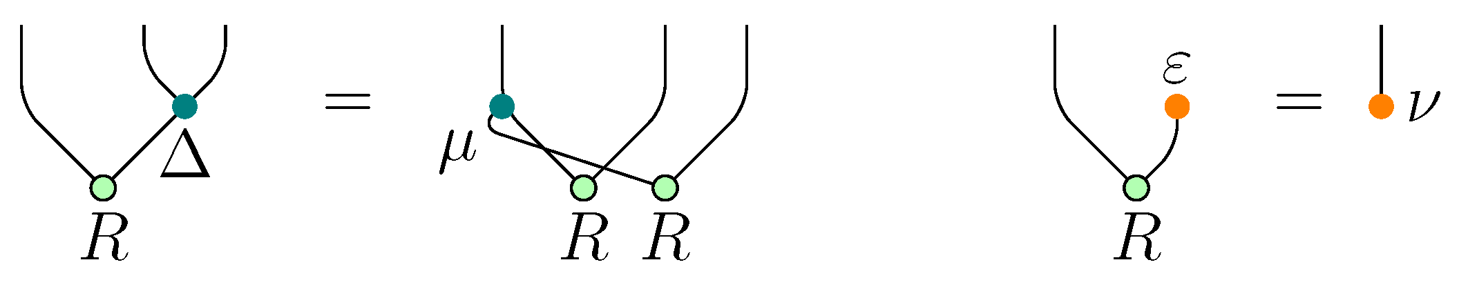
Definition 2.14. A morphism is called a weak R-matrix for a UAA and a coUAA object in if (cf. Figure 11)
Figure 11.
Axioms for a weak R-matrix.

One can informally interpret the first two conditions by saying that R provides a duality between the UAA on the right and the coUAA on the left.
Remark 2.15. If the weak R-matrix is invertible, then axiom 2 is a consequence of 1: apply to both sides, then multiply by on the left and apply
We also need the following notion:
Definition 2.16. A strong R-matrix is a weak R-matrix satisfying two additional axioms (Figure 12):
- 1’
- 2’
Figure 12.
Additional axioms for a strong R-matrix.
A strong R-matrix satisfies all usual R-matrix axioms by definition. For invertible R-matrices, arguments similar to those from Remark 2.15 show that axiom 2’. is a consequence of 1’., hence the notions of strong and usual R-matrix coincide.
As it was hinted before Definition 2.14, a weak R-matrix for H allows to upgrade a module structure over the algebra H into a Yetter-Drinfel′d module structure:
Theorem 3. Take a UAA and a coUAA object in equipped with a weak R-matrix
- For any left H-module the data form a left-right YD module over
- For any two H-modules (and hence YD modules) and the morphism from Equation (20) coincides with from Equation (24) and, for defines a braiding for the object M in
- The category can be seen as a full subcategory of via the inclusion
- If H is a bialgebra and R is a strong R-matrix, then the functor is braided monoidal.
Proof.
- The first two conditions from the definition of weak R-matrix guarantee that defines a coUAA comodule, while the last one implies the YD compatibility (YD).
- The equality of the two morphisms follows from the choice of The fact that is a braiding was noticed in Remark 2.13.
- We have seen in point 1 that is well defined on objects. Further, using the definition of and the naturality of one checks that a morphism in respecting module structures necessarily respects comodule structures defined by Thus is well defined, full and faithful on morphisms.
- Let us now show that, under the additional conditions of this point, respects monoidal structures. Take two H-modules and The H-module structure on is given by Equation (16). The functor transforms it into a YD module over with as H-comodule structureNow in the tensor product of and has an H-module structure given by and an H-comodule structure given by Equation (22):The reader is advised to draw diagrams in order to better follow these calculations. Now, axiom 1’. from the definition of a strong R-matrix is precisely what is needed for the two YD structures on to coincide.A similar comparison of the standard H-comodule structure on the unit object of with the one induced by R shows that they coincide if and only if axiom 2’. is verified.Point 2 shows that also respects braidings, allowing one to conclude. ☐
Note that in Point 2, is a morphism in and not in in general, since the H-module structure on is not even defined if H is not a bialgebra.
In the proof of the theorem one clearly sees that the full set of strong R-matrix axioms is necessary only if one wants to construct braided monoidal categories, while the notion of weak R-matrix suffices if one is interested in the “local” structure of objects in (in particular, in solutions to the YBE) only.
The relations between different structures from the above theorems can be presented in the following charts (in each of them one starts with a UAA and a coUAA H and a morphism ):
![Axioms 02 00443 i001]()

Observe that if one disregards all the structural issues and limits oneself to the search of solutions to the YBE, one obtains that the only condition that should be imposed on R so that Equation (20) becomes a braiding is the following:
where and * stands for the multiplication on defined by a formula analogous to Equation (18). This relation is sometimes called algebraic, or quantum, Yang-Baxter equation. Other authors however reserve this term for (YBE).
We finish by showing that in the Hopf algebra case, which is the most common in literature, the invertibility of a weak R-matrix is automatic:
Proposition 2.17. If a Hopf algebra H with the antipode s is endowed with a weak R-matrix then
defines an inverse for in the sense of Equation (19).
Proof. Apply or to both sides of the axiom 1 from the definition of weak R-matrix. Axiom 2 and the definition (s) of the antipode allow one to conclude. ☐
3. Yetter-Drinfeld Modules and the Yang-Baxter Equation: The Story Continued
3.1. Braided Systems
In order to describe further connections between Yetter-Drinfeld modules and the Yang-Baxter equation, the following notion from [8] will be useful:
Definition 3.1.
- ➛
- A braided system in a monoidal category is an ordered finite family of objects in endowed with a braiding, i.e., morphisms for satisfying the colored Yang-Baxter equation (= cYBE)on all the tensor products with (Here stands for ) Such a system is denoted by or briefly
- ➛
- The rank of a braided system is the number r of its components.
- ➛
- A braided morphism between two braided systems in of the same rank r is a collection of morphisms respecting the braiding, i.e.,
- ➛
- The category of rank r braided systems and braided morphisms in is denoted by
This notion is a partial generalization of that of braided object in in the sense that a braiding is defined only on certain couples of objects (which is underlined in the definition).
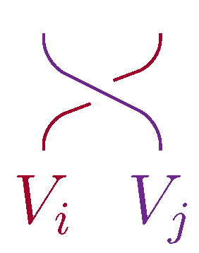
Graphically, the component of a braiding is depicted on Figure 13. According to the definition, one allows a strand to overcross only the strands colored with a smaller or equal index
Figure 13.
A braiding component.

Observe that each component of a braided system is a braided object in
Various examples of braided systems coming from algebraic considerations are presented in [8]. Different aspects of those systems are studied in detail there, including their representation and homology theories, generalizing usual representation and homology theories for basic algebraic structures.
In the next section we will describe a rank 3 braided system constructed from a Yetter-Drinfeld module over a finite-dimensional -linear bialgebra. The braiding on this system captures all axioms of the YD module structure. Several components of this braiding are inspired by the braiding from Equation (28).
3.2. Yetter-Drinfeld Module ⟼ Braided System
In this section we work in the category of -vector spaces and -linear maps, endowed with the usual tensor product over with the unit and with the flip
as symmetric braiding. Note however that one could stay in the general setting of a symmetric category and replace the property “finite-dimensional” with “admitting a dual” in what follows.
Recall the classical Sweedler’s notation without summation sign for comultiplications and coactions in used here and further in the paper:
We now describe by giving explicit formulas a braided system constructed from an arbitrary YD module. In Section 3.4 this construction will be explained from a more conceptual viewpoint.
Theorem 4.
Let H be a finite-dimensional -linear bialgebra, and let M be a Yetter-Drinfeld module over Then the rank 3 system can be endowed with the following braiding:
Here the signs for multiplication morphisms in H and as well as for the H-action on are omitted for simplicity. Further, denotes the unit of i.e., for all
Multiplication, comultiplication and other structures on used in the theorem are obtained from those on H by duality. For instance,
See [8] for some comments on an alternative definition of the duality between and which gives a slightly different formula for more common in literature.
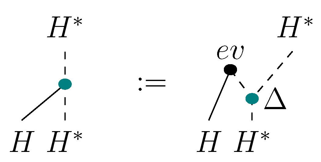
The multiplication on is graphically depicted on Figure 14. Here and afterwards dashed lines stand for and denotes one of the evaluation maps
Figure 14.
Dual structures on via the “rainbow” duality.

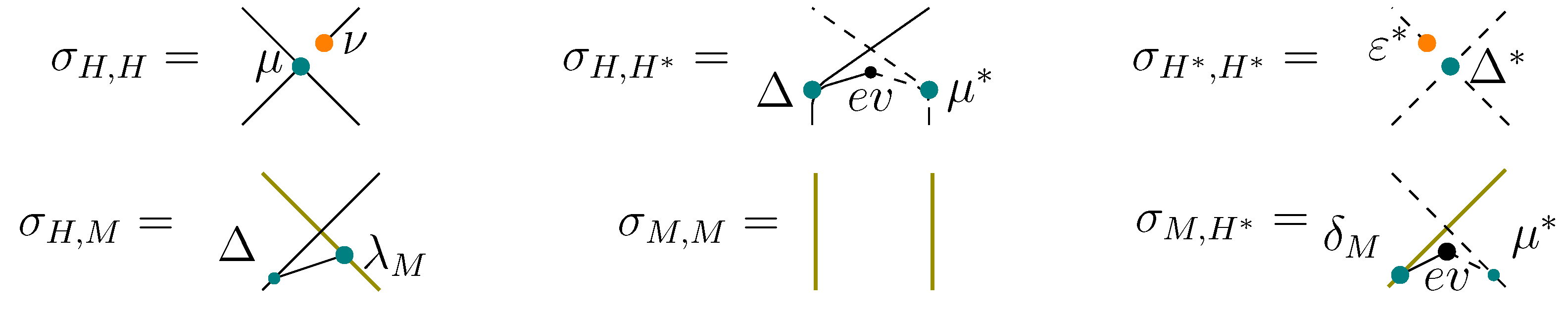
All components of the braiding from the theorem are presented on Figure 15.
Figure 15.
A braiding for the system .
In order to prove the theorem, one can simply verify by tedious but straightforward computations the instances of the cYBE involved in the definition of rank 3 braided system. A more conceptual proof will be given in the more general setting of Section 3.3 and Section 3.4 (cf. Example 3.11). In subsequent sections we will also study functoriality, precision and homology questions for this braided system.
3.3. Yetter-Drinfeld Systems: Definition and Braided Structure
We introduce here the notion of Yetter-Drinfeld system in a symmetric category and show how to endow it with a braiding. The braided system from Section 3.2 turns out to be a particular case of this general construction. In Section 3.4 we will consider other particular cases, namely a braided system encoding the bialgebra structure (cf. [8]) and a braided system of several Yetter-Drinfeld modules over a common bialgebra The latter will lead to a “braided” interpretation of the monoidal structures on the category (Section 3.6).
Let an object H in be endowed with a UAA structure and a coUAA structure a priori not compatible.
Definition 3.2.
- ➛
- A (left-right) Yetter-Drinfeld module algebra over H is the datum of a UAA structure and a YD structure on an object V in such that μ and ν are morphisms of YD modules (see Equations (26), (27) and (17), (23) for the H-(co)module structure of and of ):
- ➛
- The category of YD module algebras over H in (with as morphisms those which are simultaneously UAA and YD module morphisms) is denoted by
- ➛
- Omitting the comodule structure δ from the definition, one gets the notion of H-module algebra. H-comodule algebras are defined similarly.
The name -module algebra would be more appropriate than H-module algebra since we use the twisted compatibility condition (36). However we opt for the simpler notation since it causes no confusion in what follows.
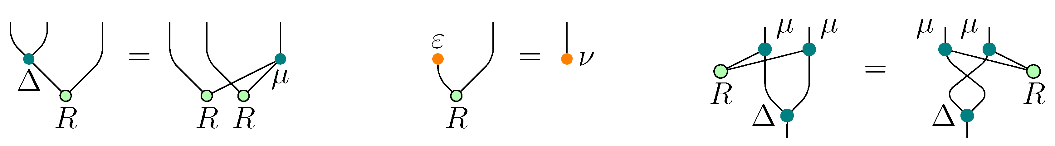
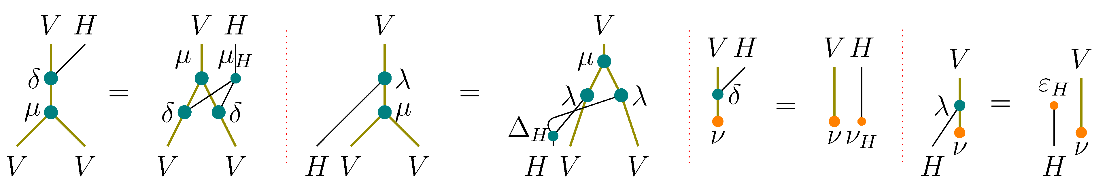
For the reader’s convenience, we give in Figure 16 a graphical form of the compatibility relations (35)–(38). Here and afterwards we use thick colored lines for the module V, and thin black lines for
Figure 16.
Compatibilities between UAA and YD structures.

Definition 3.3. A (left-right) Yetter-Drinfeld system over H (=H-YD system) in is an ordered finite family of objects endowed with the following structure:
- is an H-comodule algebra;
- is an H-module algebra;
- is a YD module algebra over H for all
Now we show how to endow a YD system with a braiding:
Theorem 5. A braiding can be defined on a Yetter-Drinfeld system over H by
The components of this braiding with are invertible if H is a Hopf algebra.
In order to prove the theorem, the following result from [8] will be useful:
Proposition 3.4. Take r UAAs in a monoidal category and, for each couple of subscripts take a morphism natural with respect to and (in the sense of a multi-object version of Equations (10) and (11)). The following statements are then equivalent:
- The morphismscomplete the ’s into a braided system structure on
- Each is natural with respect to and (in the sense of a multi-object version of Equations (8) and (9)) and, for each triple the ’s satisfy the colored Yang-Baxter equation on
We call braided systems described in the proposition braided systems of UAAs. In [8] this structure was shown to be equivalent to that of a multi-braided tensor product of UAAs.
The associativity braidings from Equation (39) were introduced in [13], where they were shown to encode the associativity (in the sense that the YBE for is equivalent to being associative, if one imposes that is a unit for ) and to capture many structural properties of the latter. We denote them by Observe that they are highly non-invertible in general.
Remark 3.5. Some or all of the morphisms in the proposition can be replaced with their right versions
Proof of the theorem. First notice that the compatibility conditions (37) and (38) between the units of the ’s and the H-(co)module structures on the ’s (cf. two last pictures on Figure 16) ensure that is natural with respect to units. In order to deduce the theorem from Proposition 3.4, it remains to check the following two conditions:
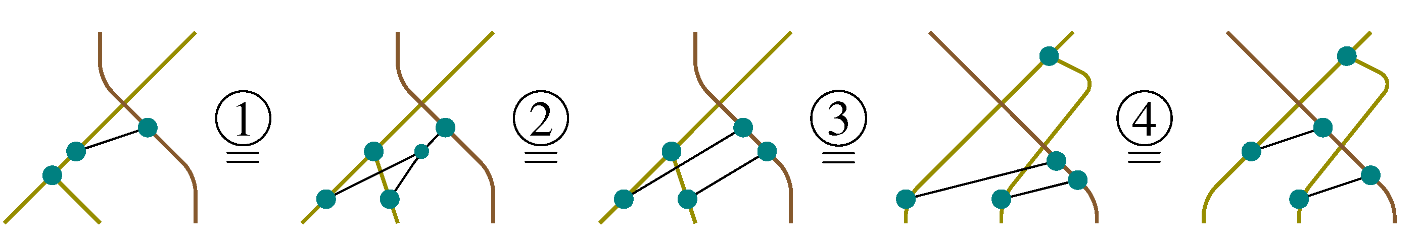
- The naturality of with respect to and for each coupleFigure 17 contains a graphical proof of the naturality with respect to the case of being similar. Labels etc. are omitted for compactness.
Figure 17.
Naturality with respect to : a graphical proof.

Here we use:
- ①
- the compatibility (35) between and (cf. Figure 16, picture 1);
- ②
- the definition of H-module for ;
- ③
- the naturality of the symmetric braiding c of ;
- ④
- the naturality and the symmetry (5) of c.
- 2.
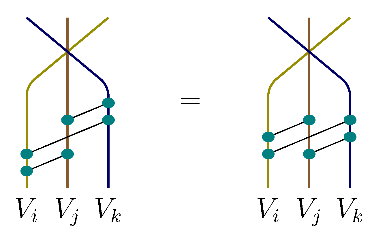
- Condition (cYBE) on for each tripleDue to the naturality of this condition is equivalent to the one graphically presented on Figure 18.
Figure 18.
Yang-Baxter equation for Yetter-Drinfeld modules.

To prove this, one needs
- ➛
- the defining property of right H-comodule for
- ➛
- the defining property of left H-module for
- ➛
- the Yetter-Drinfeld property for
As for the invertibility statement, if H is a Hopf algebra, then the inverse of can be explicitely given by the formula
Remark 3.6.
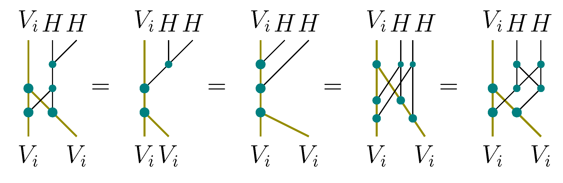
No compatibility between the algebra and coalgebra structures on H are demanded explicitly. However, other properties of a YD system dictate that H should be not too far from a bialgebra, at least as far as (co)actions are concerned. This statement is made concrete and is proved (in the H-comodule case) in Figure 19; cf. Figure 4 for the definition of bialgebra.
Figure 19.
Almost a bialgebra.

3.4. Yetter-Drinfeld Systems: Examples
The examples of H-YD systems we give below contain usual YD modules over a priori without a UAA structure. In the following lemma we explain how to overcome this lack of structure by introducing a formal unit into a YD module:
Lemma 3.7.
Let be a YD module over a UAA and coUAA H in a symmetric additive category This YD module structure can be extended to as follows:
Moreover, combined with the trivial UAA structure on :
this extended YD module structure turns M into an H-YD module algebra.
Proof.
Direct verifications. ☐
We need to be additive in order to ensure the existence of direct sums and zero morphisms. Our favorite category is additive.
In what follows we mostly work with YD modules admitting moreover a compatible UAA structure; the lemma shows that this assumption does not reduce the generality of our constructions.
Everything is now ready for our main example of H-YD systems. Recall Sweedler’s notation (31) and (32).
Proposition 3.8.
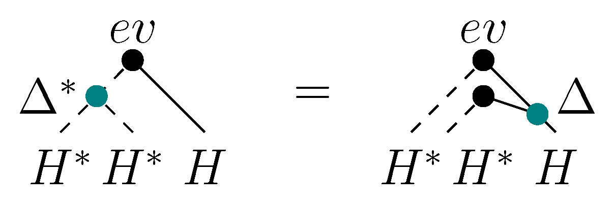
Let H be a finite-dimensional -linear bialgebra, and let be Yetter-Drinfeld module algebras over Consider H itself as a UAA via morphisms and and as an H-comodule via Further, consider its dual space as a UAA via dual morphisms and and as an H-module via
(cf. Figure 20). These structures turn the family into an H-YD system.
Figure 20.
The action of H on H*.
Proof.
Almost all axioms from Definition 3.3 are automatic. One should check only the following points:
- ➛
- the H-comodule structure on H is compatible with the UAA structure ;
- ➛
- the map Equation (40) indeed defines an H-action on ;
- ➛
- the H-module structure Equation (40) on is compatible with the UAA structure .
These straightforward verifications use bialgebra axioms and the definition of dual morphisms. They are easily effectuated using the graphical calculus. ☐
Applying Theorem 5 to the H-YD system from Proposition 3.8, and choosing braiding component for and the ’s, and its right version for H (cf. Remark 3.5), one obtains the following braided system:
Corollary 3.9.
In the settings of Proposition 3.8, the system can be endowed with the following braiding:
Notations analogous to those from Theorem 4 are used here.
See Figure 9 and Figure 15 for a graphical presentation of the components of the braiding from the corollary. Notation will further be used for this braiding.
The simplest particular cases of the corollary already give interesting examples:
Example 3.10.
In the extreme case one gets the braiding on the system studied in [8], where it was shown that:
- ➛
- it encodes the bialgebra structure (e.g., the cYBE on or on is equivalent to the main bialgebra axiom (15));
- ➛
- it allows to construct a fully faithful functorwhere is the category of finite-dimensional bialgebras and bialgebra isomorphisms (hence notation ) in and is the category of rank 2 braided systems and their isomorphisms in endowed with some additional structure (hence notation );
- ➛
- the invertibility of the component of this braiding is equivalent to the existence of the antipode for H;
- ➛
- ➛
- the braided homology theory for this system (cf. Section 3.7) includes the Gerstenhaber-Schack bialgebra homology, defined in [20].
Example 3.11.
The case gives a braiding on the system for a YD module algebra M over Now observe that one can substitute the component of with the trivial one, since the instances of the cYBE involving two copies of M (which are the only instances affected by the modification of ) become automatic. Moreover, with this new the UAA structure on M is no longer necessary. One thus obtains a braiding on for any H-YD module which coincides with the one in Theorem 4. This gives an alternative proof of that theorem.
Example 3.12.
If M is just a module algebra, one can extract a braided system from the construction of the previous example. Studying braided differentials for this system (cf. Section 3.7), one recovers the deformation bicomplex of module algebras, introduced by D. Yau in [21]. Note that in this example H need not be finite-dimensional.
Example 3.13.
The argument from example 3.11 also gives a braiding on the system for H-YD modules a priori without UAA structures. This braiding is obtained by replacing all the ’s from Corollary 3.9 with the trivial ones, It is denoted by
3.5. Yetter-Drinfeld Systems: Properties
Now let us study several properties of the braiding from Corollary 3.9, namely its functoriality and the precision of encoding YD module algebra axioms.
Proposition 3.14.
In the settings of Proposition 3.8, one has a faithful functor
Moreover, if a braided morphism from to has the form and if the ’s respect units (in the sense of Equation (7)), then all the are morphisms in
Proof.
Corollary 3.9 says that the functor is well defined on objects. It remains to study the compatibility condition (29) for the collection and each component of the braiding
- On and condition (29) trivially holds true.
- On condition (29) readswhich, due to Equation (7), becomesBut this is equivalent to respecting multiplication:(compose with on the left to get the less evident application), i.e., in the presence of Equation (7), to being a UAA morphism.
- On condition (29) readswhich simplifies asThis is equivalent to respecting the H-module structure:(compose with on the left to get the less evident application).
- Similarly, on condition (29) is equivalent to respecting the H-comodule structure.
- Condition (29) holds true on if respects the H-module structures and respects the H-comodule structures.
The reader is advised to draw diagrams in order to better follow the proof.
This analysis shows that is well defined on morphisms. Moreover, it shows that if a braided morphism from to has the form and if the ’s respect units, then all the are simultaneously morphisms of UAAs (point 2 above), of H-modules (point 3) and of H-comodules (point 4), which precisely means that they are morphisms in
The faithfulness of the functor is tautological. ☐
Remark 3.15.
The second statement of the proposition allows to call the functor “essentially full”. A precise description of can be obtained using the results recalled in Example 3.10. Namely, if one imposes some additional restrictions (α and β should be invertible and respect the units, the ’s should respect units as well), then
- ➛
- α is a bialgebra automorphism, and coinsides with ;
- ➛
- each is a UAA morphism;
- ➛
- α and the ’s are compatible with the YD structures on the ’s and ’s:
Remark 3.16.
Following Example 3.13, one gets a similar “essentially full” and faithful functor
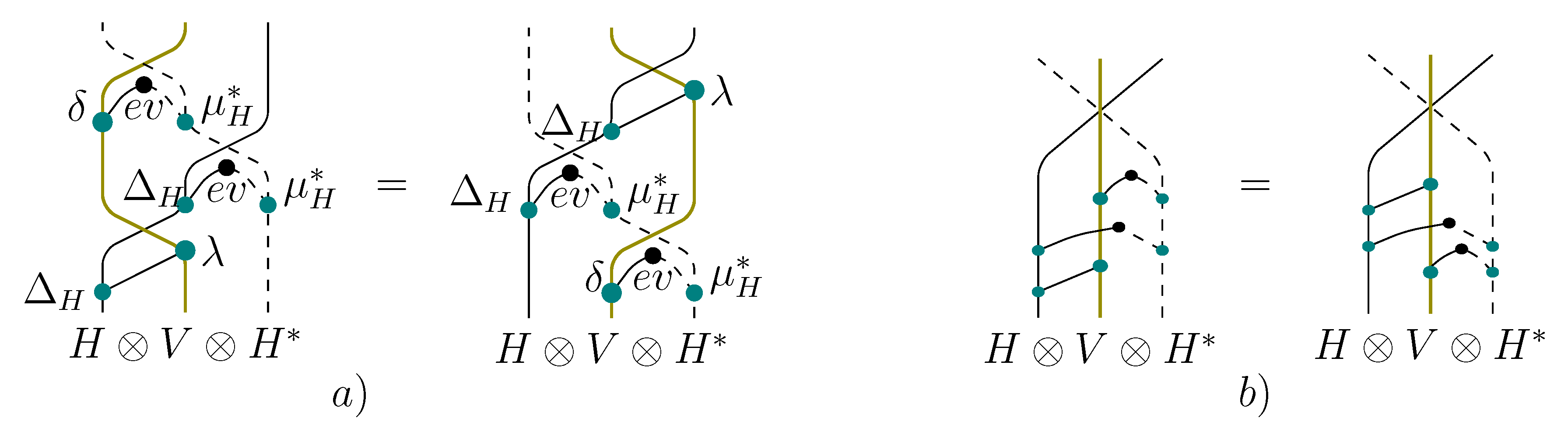
We next show that each instance of the cYBE for the braiding corresponds precisely to an axiom from the Definition 3.2 of YD module algebra structure, modulo some minor normalization constraints. We thus obtain a “braided” interpretation of each of these axioms, extending the classical “braided” interpretation of the YD compatibility condition (YD) (Corollary 2.11).
Proposition 3.17.
Take a finite-dimensional -linear bialgebra a vector space V over and morphisms a priori satisfying no compatibility relations. Consider the collection of σ’s defined in Corollary 3.9 (for ). One has the following equivalences:
- cYBE for ⟺ YD compatibility condition (YD) for
- cYBE for ⟺λ defines an H-module.Here one supposes that acts via λ by identity (in the sense of Equation (13)).
- cYBE for ⟺δ defines an H-comodule.Here one supposes that coacts via δ by identity (in the sense dual to Equation (13)).
- cYBE for ⟺λ respects the multiplication μ (in the sense of Equation (36)).Here one supposes λ to respect ν (in the sense of Equation (38)).
- cYBE for ⟺δ respects the multiplication μ (in the sense of Equation (35)).Here one supposes δ to respect ν (in the sense of Equation (37)).
- cYBE for associativity of
Proof.
We prove only the first equivalence here, the other points being similar.
The cYBE for is graphically depicted on Figure 21(a). Using the naturality of one transforms this into the diagram on Figure 21(b). Applying to both sides and using the definition of in terms of one gets precisely (YD).
Figure 21.
cYBE for ⟺ (YD).

3.6. Tensor Product of Yetter-Drinfeld Modules
The aim of this section is to explain the definition (26) and (27) of tensor product of YD modules from the braided point of view, using the braided interpretation of YD structure presented in Proposition 3.17.
Start with an easy general observation.
Lemma 3.18.
Let be a rank 4 braided system in a monoidal category A braiding can then be defined for the rank 3 system in the following way:
- ➛
- keep and from the previous system;
- ➛
- put ;
- ➛
- define
Proof.
The instances of the cYBE not involving hold true since they were true in the original braided system. Those involving at least twice are trivially true. The remaining instances (those involving exactly once) are verified by applying the instances of the cYBE coming from the original braided system several times. ☐
Certainly, this gluing procedure can be applied in a similar way to any two or more consecutive components in a braided system of any rank.
Applying the gluing procedure to the braided system from Example 3.13 () and slightly rewriting the braiding obtained (using the coassociativity of H and of ), one gets
Lemma 3.19.
Given YD modules and over a finite-dimensional -linear bialgebra one has the following braiding on :
where denotes the action (40) of H on and and are defined by Equations (26) and (27).
Now plug and (and arbitrary μ and ν) into Proposition 3.17. The preceding lemma ensures the cYBE on and (since the corresponding components of from the proposition and from the lemma coincide). The equivalences from the proposition then allow to conclude:
Corollary 3.20.
Given YD modules and over a finite-dimensional -linear bialgebra the morphisms and defined by Equations (26) and (27) endow with a YD module structure.
One thus obtains a more conceptual way of “guessing” the correct definition of tensor product for YD modules.
3.7. Braided Homology: A Short Review
In this section we recall the homology theory for braided systems developed in [8] (see also [13] for the rank i.e., braided object, case). In the next section we apply this general theory to the braided system constructed from a YD module in Theorem 4.
We first explain what we mean by a homology theory for a braided system in an additive monoidal category :
Definition 3.21.
- ➛
- A degree differential for a collection of objects in is a family of morphisms satisfying
- ➛
- A bidegree bidifferential for a collection of objects in consists of two families of morphisms satisfying
- ➛
- An ordered tensor product for is a tensor product of the form
- ➛
- The degree of such a tensor product is the sum
- ➛
- The direct sum of all ordered tensor products of degree n is denoted by
- ➛
- A (bi)degree (bi)differential for is a (bi)degree (bi)differential for
One also needs the “braided” notion of character, restricting in particular examples to the familiar notions of character for several algebraic structures such as UAAs and Lie algebras (cf. [13]).
Definition 3.22.
A braided character for is a rank r braided system morphism from to
In other words, it is a collection of morphisms satisfying the compatibility condition
We now exhibit a bidegree bidifferential for an arbitrary braided system endowed with braided characters; see [8] for motivations, proofs, a multi-quantum shuffle interpretation and properties of this construction.
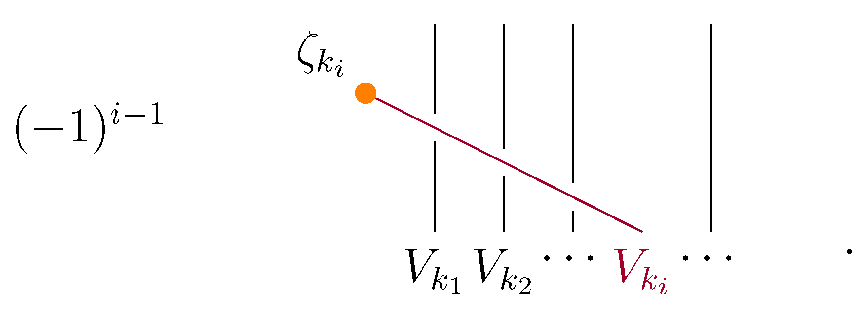
Theorem 6.
Take a braided system in an additive monoidal category equipped with two braided characters and The families of morphisms
from to define a bidegree tensor bidifferential. Here the stars * mean that each time one should choose the component of or corresponding to the ’s on which it acts. Further, notation (1) for superscripts is used.
Pictorially, for example is a signed sum (due to the use of the negative braiding ) of the terms presented on Figure 22. The sign can be interpreted via the intersection number of the diagram.
Figure 22.
Multi-braided left differential.

Corollary 3.23.
Any -linear combination of the families and from the theorem is a degree differential.
Definition 3.24.
The (bi)differentials from the above theorem and corollary are called multi-braided.
Remark 3.25.
- ➛
- The constructions from the theorem are functorial.
- ➛
- Applying the categorical duality to this theorem, one gets a cohomology theory for
- ➛
- The braided bidifferentials can be shown to come from a structure of simplicial (or, more precisely, cubical) type.
3.8. Braided Homology of Yetter-Drinfeld Modules
Let us now apply Theorem 6 to the braided system from Theorem 4. As for braided characters, we use the following ones:
Lemma 3.26.
Morphisms and are braided characters for the braided system from Theorem 4.
These braided characters are abusively denoted by and in what follows.
Proof.
We prove the statement for only, the one for being similar.
Both sides of Equation (42) are identically zero for the morphisms from the lemma, except for the case corresponding to In this latter case, Equation (42) becomes
which follows from the fact that is an algebra morphism (cf. the definition of bialgebra). ☐
In what follows, the letters always stay for elements of – for elements of the pairing is the evaluation; the multiplications and on H and respectively, as well as H- and -actions, are denoted by · for simplicity. We also use higher-order Sweedler’s notations of type
Further, we omit the tensor product sign when this does not lead to confusion, writing for instance
Using these notations, one can write down explicite braided differentials for a YD module:
Proposition 3.27.
Take a Yetter-Drinfeld module over a finite-dimensional -linear bialgebra There is a bidegree bidifferential on given by
Proof.
These are just the constructions from Theorem 6 applied to the braided system from Theorem 4 and braided characters and Note that we restricted the differentials from to which is possible since both and are zero on ☐
Remark 3.28.
In fact the differentials and define a double complex structure on graduated by putting
In order to get rid of the classical contracting homotopies of type
we now try to “cycle” this bidifferential, in the spirit of Hochschild homology for algebras or Gerstenhaber-Schack homology for bialgebras.
Concretely, take a YD module and a finite-dimensional YD module over Our aim is to endow the graded vector space
with a bidifferential extending that from Proposition 3.27.
First, note that the “rainbow” duality between H and (cf. (33) or Figure 14) graphically corresponds to an angle π rotation. Since the notions of bialgebra and YD module are centrally symmetric (cf. Remark 2.10), one gets the following useful property:
Lemma 3.29.
Take a finite-dimensional YD module over a finite dimensional bialgebra Then is a YD module over
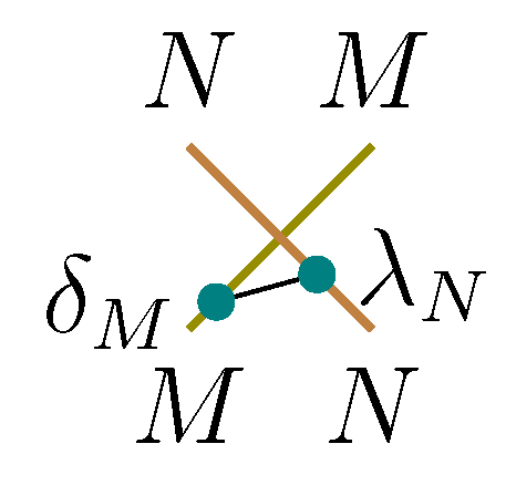
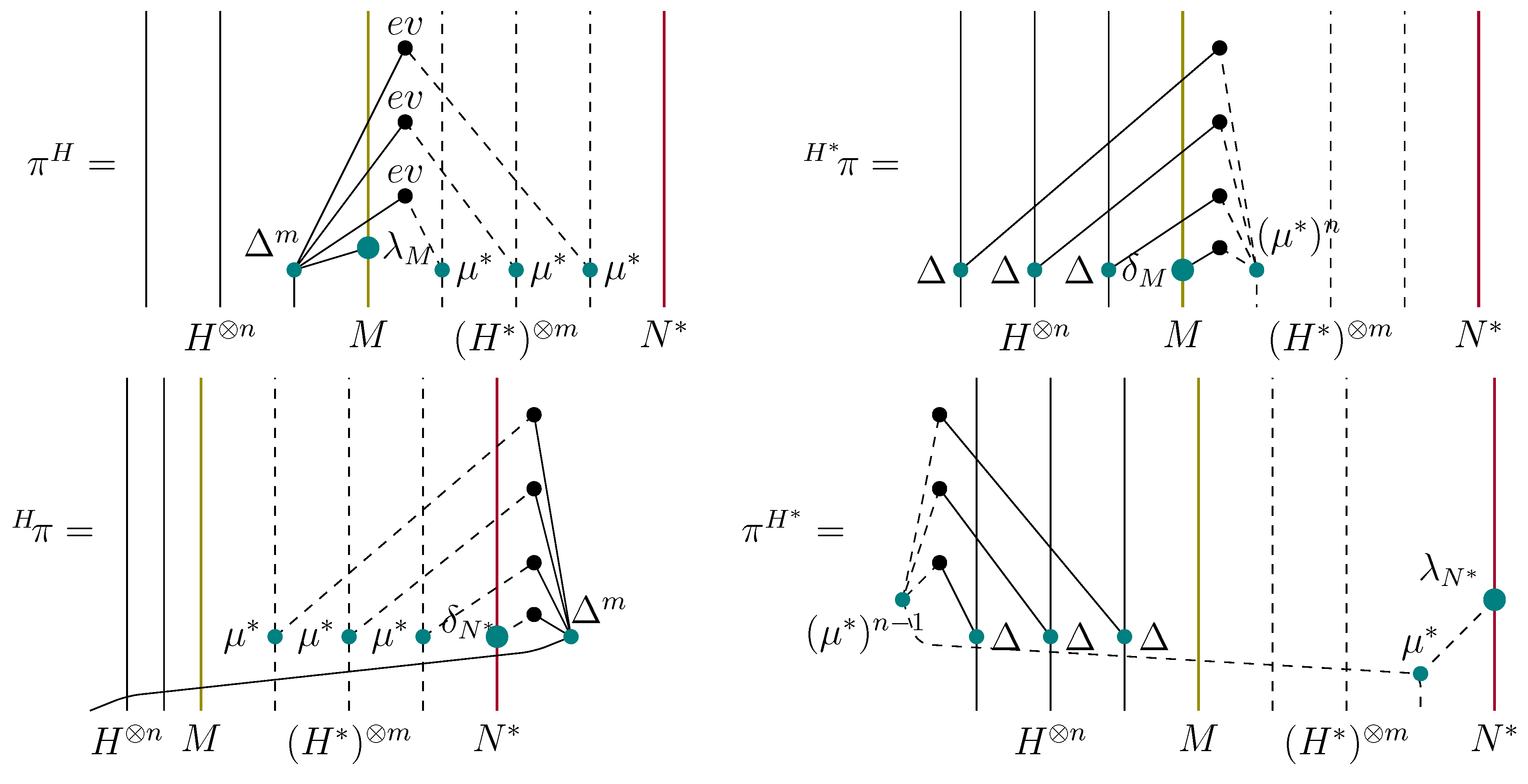
Further, inspired by the formulas from Proposition 3.27, consider the following morphisms from to or :
These applications are presented on Figure 23. We use notation
and similarly for
Figure 23.
Components of YD module homology.

These morphisms can be interpreted in terms of “braided” adjoint actions, as it was done for the bialgebra case in [8].
At last, recall the classical bar and cobar differentials:
Everything is now ready for presenting an enhanced version of Proposition 3.27:
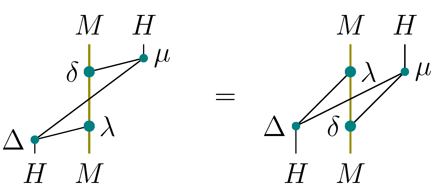
Theorem 7.
Given a YD module M and a finite-dimensional YD module N over a finite-dimensional bialgebra H in one has four bidegree bidifferentials on presented in the lines of Table 1.

 |
The signs etc. here are those one chooses on the component of
Substituting the graded vector space we work in with its alternative version (as it was done for example in [22]), we obtain (the dual of a mirror version of) the deformation cohomology for YD modules, defined by F. Panaite and D. Ştefan in [14]. We have thus developed a conceptual framework for this cohomology theory, replacing case by case verifications (for instance, when proving that one has indeed a bidifferential) with a structure study, facilitated by graphical tools.
3.9. Proof of Theorem 7
Morphisms and are well known to be differentials; this can be easily verified by direct calculations, or using the rank 1 braided systems and , cf. [13]. Further, they affect different components of (namely, and ) and thus commute. The sign guarantees the anti-commutation. This proves that the first line of the table contains a bidegree bidifferential.
The assertion for the second line follows from Proposition 3.27, since
To prove the statement for the third line, note that the dual (in the sense of Lemma 3.29) version of Proposition 3.27 gives a bidifferential on and hence (by tensoring with ) on Identifying the latter space with via the flip Equation (30) and keeping notation for the bidifferential induced on this new space, one calculates
Multiplying by and by and checking that this does not break the anti-commutation, one recovers the third line of the table.
We start the proof for the fourth line with a general assertion:
Lemma 3.30.
Take an abelian group endowed with an operation · distributive with respect to Then, for any such that
one has
Proof.
☐
Now take with the usual addition and the operation composition (for proving that the two morphisms from the fourth line of our table are differentials), or the operation (for proving that the two morphisms anti-commute). The information from the first three lines and Lemma 3.31 allow to apply Lemma 3.30 to sextuples and (for the operation ∘), and (for the operation ⋄), where
One thus gets the fourth line of the table.
Lemma 3.31.
The endomorphisms and of pairwise commute.
Proof.
The commutation of and follows from the coassociativity of (this is best seen in Figure 23). The pair is treated similarly.
The commutation of and follows from their interpretation as parts of a precubical structure (cf. [13]), or by a direct computation. The pair is treated similarly.
The case of the pair demands more work.
Denote by a version of which “forgets” the rightmost component of :
Similarly, denote by a version of which “forgets” the rightmost component of H:
Further, put
Observe that θ is precisely the difference between the π’s and their reduced versions :
Moreover, one has
since and modify different components of (the hat (dis)appears when these morphisms switch because kills the rightmost copy of and kills the rightmost copy of ). Therefore,
hence the desired commutation.
The pair is treated similarly. ☐
Remark 3.32.
Lemma 3.31 actually contains more than needed for the proof of the theorem. We prefer keeping its full form and checking the commutation of all the pairs of morphisms for completeness.
Acknowledgements
The author is grateful to the Referees for the comments allowing to improve the presentation of the paper, and to Marc Rosso and Józef Przytycki for stimulating discussions.
Conflicts of Interest
The author declares no conflicts of interest.
References
- Drinfel’d, V.G. Quantum Groups. In Proceedings of the International Congress of Mathematicians, Berkeley, CA, USA, 1986; American Mathematical Society: Providence, RI, USA, 1987; pp. 798–820. [Google Scholar]
- Yetter, D.N. Quantum groups and representations of monoidal categories. Math. Proc. Camb. Philos. Soc. 1990, 108, 261–290. [Google Scholar] [CrossRef]
- Woronowicz, S.L. Solutions of the braid equation related to a Hopf algebra. Lett. Math. Phys. 1991, 23, 143–145. [Google Scholar] [CrossRef]
- Montgomery, S. Hopf Algebras and Their Actions on Rings; CBMS Regional Conference Series in Mathematics; Published for the Conference Board of the Mathematical Sciences: Washington, DC, USA, 1993; Volume 82, p. xiv+2388. [Google Scholar]
- Takeuchi, M. Survey of Braided Hopf Algebras. In New Trends in Hopf Algebra Theory (La Falda, 1999); American Mathematical Society: Providence, RI, USA, 2000; Volume 267, pp. 301–323. [Google Scholar]
- Joyal, A.; Street, R. Braided tensor categories. Adv. Math. 1993, 102, 20–78. [Google Scholar] [CrossRef]
- Lebed, V. Braided Objects: Unifying Algebraic Structures and Categorifying Virtual Braids. Ph.D. Thesis, Université Paris, Paris, France, 2012. [Google Scholar]
- Lebed, V. Braided systems, Multi-Braided Tensor Products and Bialgebra Homologies. 2013. arXiv:1305.0944. arXiv.org e-Print archive. Available online: http://arxiv.org/abs/1305.0944 (accessed on 4 September 2013).
- Hlavatý, L.; Šnobl, L. Solution of the Yang-Baxter system for quantum doubles. Int. J. Mod. Phys. A 1999, 14, 3029–3058. [Google Scholar] [CrossRef]
- Nichita, F.F. New solutions for Yang-Baxter systems. Acta Univ. Apulensis Math. Inform. 2006, 11, 189–195. [Google Scholar]
- Brzeziński, T.; Nichita, F.F. Yang-Baxter systems and entwining structures. Commun. Algebra 2005, 33, 1083–1093. [Google Scholar] [CrossRef]
- Lambe, L.A.; Radford, D.E. Algebraic aspects of the quantum Yang-Baxter equation. J. Algebra 1993, 154, 228–288. [Google Scholar] [CrossRef]
- Lebed, V. Homologies of algebraic structures via braidings and quantum shuffles. J. Algebra 2013, 391, 152–192. [Google Scholar] [CrossRef]
- Panaite, F.; Ştefan, D. Deformation cohomology for Yetter-Drinfel′d modules and Hopf (bi)modules. Commun. Algebra 2002, 30, 331–345. [Google Scholar] [CrossRef]
- MacLane, S. Categories for the Working Mathematician; Springer-Verlag: New York, NY, USA, 1971; Volume 5, p. ix+262. [Google Scholar]
- Kassel, C. Quantum Groups; Graduate Texts in Mathematics; Springer-Verlag: New York, NY, USA, 1995; Volume 155, p. xii+531. [Google Scholar]
- Faddeev, L.; Reshetikhin, N.; Takhtajan, L. Quantum Groups. In Braid Group, Knot Theory and Statistical Mechanics; World Science Publication: Teaneck, NJ, USA, 1989; Volume 9, pp. 97–110. [Google Scholar]
- Faddeev, L.D.; Reshetikhin, N.Y.; Takhtajan, L.A. Quantization of Lie Groups and Lie algebras. In Algebraic Analysis; Academic Press: Boston, MA, USA, 1988; Volume I, pp. 129–139. [Google Scholar]
- Radford, D.E. Solutions to the quantum Yang-Baxter equation and the Drinfel′d double. J. Algebra 1993, 161, 20–32. [Google Scholar] [CrossRef]
- Gerstenhaber, M.; Schack, S.D. Bialgebra cohomology, deformations, and quantum groups. Proc. Natl. Acad. Sci. USA 1990, 87, 478–481. [Google Scholar] [CrossRef]
- Yau, D. Deformation bicomplex of module algebras. Homol. Homotopy Appl. 2008, 10, 97–128. [Google Scholar] [CrossRef]
- Mastnak, M.; Witherspoon, S. Bialgebra cohomology, pointed Hopf algebras, and deformations. J. Pure Appl. Algebra 2009, 213, 1399–1417. [Google Scholar] [CrossRef]
© 2013 by the authors; licensee MDPI, Basel, Switzerland. This article is an open access article distributed under the terms and conditions of the Creative Commons Attribution license (http://creativecommons.org/licenses/by/4.0/).
Share and Cite
MDPI and ACS Style
Lebed, V. R-Matrices, Yetter-Drinfel'd Modules and Yang-Baxter Equation. Axioms 2013, 2, 443-476. https://doi.org/10.3390/axioms2030443
AMA Style
Lebed V. R-Matrices, Yetter-Drinfel'd Modules and Yang-Baxter Equation. Axioms. 2013; 2(3):443-476. https://doi.org/10.3390/axioms2030443
Chicago/Turabian StyleLebed, Victoria. 2013. "R-Matrices, Yetter-Drinfel'd Modules and Yang-Baxter Equation" Axioms 2, no. 3: 443-476. https://doi.org/10.3390/axioms2030443