Rock Classification Using Multivariate Analysis of Measurement While Drilling Data: Towards a Better Sampling Strategy

1
Department of Geoscience and Petroleum, Norwegian University of Science and Technology, Sem Saelands vei 1, N-7491 Trondheim, Norway
2
Department of Mathematical Sciences, Norwegian University of Science and Technology, Sentralbygg 2, 1034 Trondheim, Norway
*
Author to whom correspondence should be addressed.
Minerals 2018, 8(9), 384; https://doi.org/10.3390/min8090384
Submission received: 1 June 2018
/
Revised: 1 August 2018
/
Accepted: 10 August 2018
/
Published: 4 September 2018
(This article belongs to the Special Issue Geometallurgy)
Abstract
:Measurement while drilling (MWD) data are gathered during drilling operations and can provide information about the strength of the rock penetrated by the boreholes. In this paper MWD data from a marble open-pit operation in northern Norway are studied. The rock types are represented by discrete classes, and the data is then modeled by a hidden Markov model (HMM). Results of using different MWD data variables are studied and presented. These results are compared and co-interpreted with optical televiewer (OTV) images, magnetic susceptibility and spectral gamma values collected in the borehole using down-the-hole sensors. A model with penetration rate, rotation pressure and dampening pressure data show a good visual correlation with OTV image for the studied boreholes. The marble class is characterized by medium penetration rate and medium rotation pressure, whereas the intrusions are characterized by low penetration rate and medium to high rotation pressure. The fractured marble is characterized by high penetration rate, high rotation and low dampening pressure. Future research will use the presented results to develop a heterogeneity index, develop an MWD-based 3D-geology model and an improved sampling strategy and investigate how to implement this in the mine planning process and reconciliation.
1. Introduction
This paper is part of a research project focusing on the implementation of geometallurgical concepts in the industrial mineral sector of the Norwegian mining industry. A geometallurgical model is a combination of geological and mineral processing information into a spatial and predictive tool to be used in production planning and management in the mining industry [1]. These kinds of predictive models aim at taking not only grade into account when estimating key performance indicators (KPIs), but also parameters related to for example micro-scale texture information or strength and hardness variations.
The goal of this paper is to develop and test methodologies for dividing a rock mass into different rock classes based on strength and hardness variations. Measurement While Drilling (MWD) data will be used to achieve this. Strength is a material parameter quantifying a material’s ability to withstand an applied force without expressing plastic deformation. It is a mechanical property and the force and deformation are linked through the modulus of elasticity. The hardness is a physical parameter describing a material’s resistance towards abrasion. An aim is to identify and understand the influence of the important MWD data variables that can be used to identify rock strength and -hardness variations. This will render it possible to conduct geological classification of marble and other lithologies from MWD data. This can in turn be used in the development of improved sampling strategies. This do however not include a quantification nor a description of how each of the MWD-parameters can indicate either strength or hardness variations.
Large amounts of high resolution MWD data have been collected during mining, but its potential use in subsequent planning- and mining processes is not well studied. In this paper, we use hidden Markov models (HMM) and the MWD data to classify rock types in boreholes. This classification of raw material can be used to build on-line or off-line classifiers for rock classes or constitute the basis for a geological model of blasts. It can also use to develop a heterogeneity index for blocking of the blast such that each block is as homogeneous or as heterogeneous as possible. In doing so, the broader goal is to reduce ore loss and ore dilution.
2. Background
This study is based on the data collected from Brønnøy Kalk AS, a mine located near Brønnøysund in northern Norway. Figure 1 shows the map and overview of the location. Annually, the mine produces approximately 2 million tonnes of calcite marble from the open pit operation. The calcite marble is further processed into ground calcium carbonate and the final product is used as a whitening agent in paper production [2]. The carbonate deposit at Brønnøy Kalk is very heterogeneous in nature. The deposit consists of different types of marble formation and they are informally named “speckled-”, “banded-” and “impure” marble. In some areas layers of diabase, gneiss or aplite are present. These are commonly termed intrusions [3]. The different lithologies and fractures vary in hardness or strength. For instance, uniaxial compression strength (UCS) tends to be higher in diabase or gneiss than in marble [4]. According to [5] UCS of fractures is lower than intact marble. Impure marble contains thin banded layers of intrusive rocks. So hardness of impure marble considered to be higher than marble but lower than thick intrusions layers. The different lithologies also can be distinguished based on impurities and visual appearances.
At Brønnøy Kalk, a blast contains approximately 100,000 tonnes of raw material. During the normal drilling process these blasts are divided geometrically into smaller blocks or selective mining units (SMUs). Normally each SMU consists of 10–15 boreholes. One collective sample from each block is taken to a laboratory and a flotation technique used for the recovery of calcium carbonate. The quality of the final product will be determined by several outputs from the lab results such as brightness, reagent consumption and flotation loss. The good quality blocks are loaded and transported with wheeled transportation to the primary crusher, whereas marble blocks below specification are dumped at the waste dump. The sub-quality blocks will be stored temporarily and later blended with good quality blocks.
The collective sampling method has a low resolution and will homogenize and thereby smooth out the important variations. Due to the presence of a small amount of impure marble and intrusions in a block, the lab result might indicate that the average quality in a block is below the quality cut-off. This diluted “ore” will hence lead to ore loss. To sample drill cuttings from each borehole could be a very expensive solution to this challenge [6].
MWD data are collected to get relevant drilling information from the drilling rig for a systematic evaluation of the drilling performance. According to [7] the MWD data can potentially provide information regarding the mechanical properties of the rock. In the mining industry, MWD data could deliver information regarding rock mass characterization and that information can be used for long term and short term mine planning, fragmentation optimization and equipment planning for a cost-effective production [8]. MWD data can also carry important information for the blast design process by providing rock strength properties for individual blast holes and improve safety during blasting [9,10]. Similarly, drilling performance parameters are used to predict the rock quality designation (RQD) during the tunneling operation [11].
It is stated in [9,12] that the measured MWD variables can be classified as two types (1) Parameters that are independent of rock type characteristics or so-called operator controlled variables and (2) Parameters that are dependent or responsive to rock characteristics. References [8,13] state that rotation pressure, and dampening pressure are dependent on the rock characteristics. Penetration rate is depending on all of the pressures and rock characteristics. For example, if the rig increases its rotation-, feed- and percussion pressure, without having any change in rock type, the penetration rate will automatically increase. It concludes that penetration rate alone may not be a good indicator of the rock characteristics. Percussive pressure and feed pressure are not dependent on the rock characteristics but simply controlled by the rig’s system. The lower and higher extreme values in rotation pressure and dampening pressure are controlled by changing the feed and percussion pressure by the rig’s control system. The flush air pressure is very dependent on depth because more pressure is needed to flush the drill cutting from deeper sections of the borehole.
3. Materials and Methods
3.1. Data
The MWD data used in this study were collected using an Atlas-Copco T-45 drilling rig. The MWD data consist of; Depth (m), Penetration Rate (m/min), Percussion Pressure (bar), Feed Pressure (bar), Flush Air Pressure (bar), Rotation Pressure (bar) and Dampening Pressure (bar). The data are gathered in an interval of approximately every 2 cm. In addition to these MWD data, which are available in all boreholes, an optical tele-viewer image (OTV), magnetic susceptibility (MSUS), spectral gamma (SGAM) and total gamma (TGAM) are logged for some boreholes. The OTV was used to take pictures of the borehole wall. The OTV image can be used to see the fractures and their geometry and position, lithologies and orientation of any structure. MSUS is a measure of magnetic properties of a material. Similarly, SGAM identifies the existence of radioactive material inside the borehole at each depth. The SGAM measurements include the amount of existence radioactive substance such as potassium (K), thorium (Th) and uranium (U). The TGAM is aggregation of all SGAMs. The SGAM, TGAM and MSUS measures are used to indicate the mineral composition of the deposit. For instance, TGAM will be comparatively high in aplites than in diabase due to the elevated content of feldspar high in potassium. Lithologies like diabase will have higher MSUS compared to intrusions with aplite or gneiss [14]. Both MWD and logging data monitored with depth index. In this research, this borehole logging data and OTV image are used as a tool to interpret and validate the classification result from the MWD analysis.
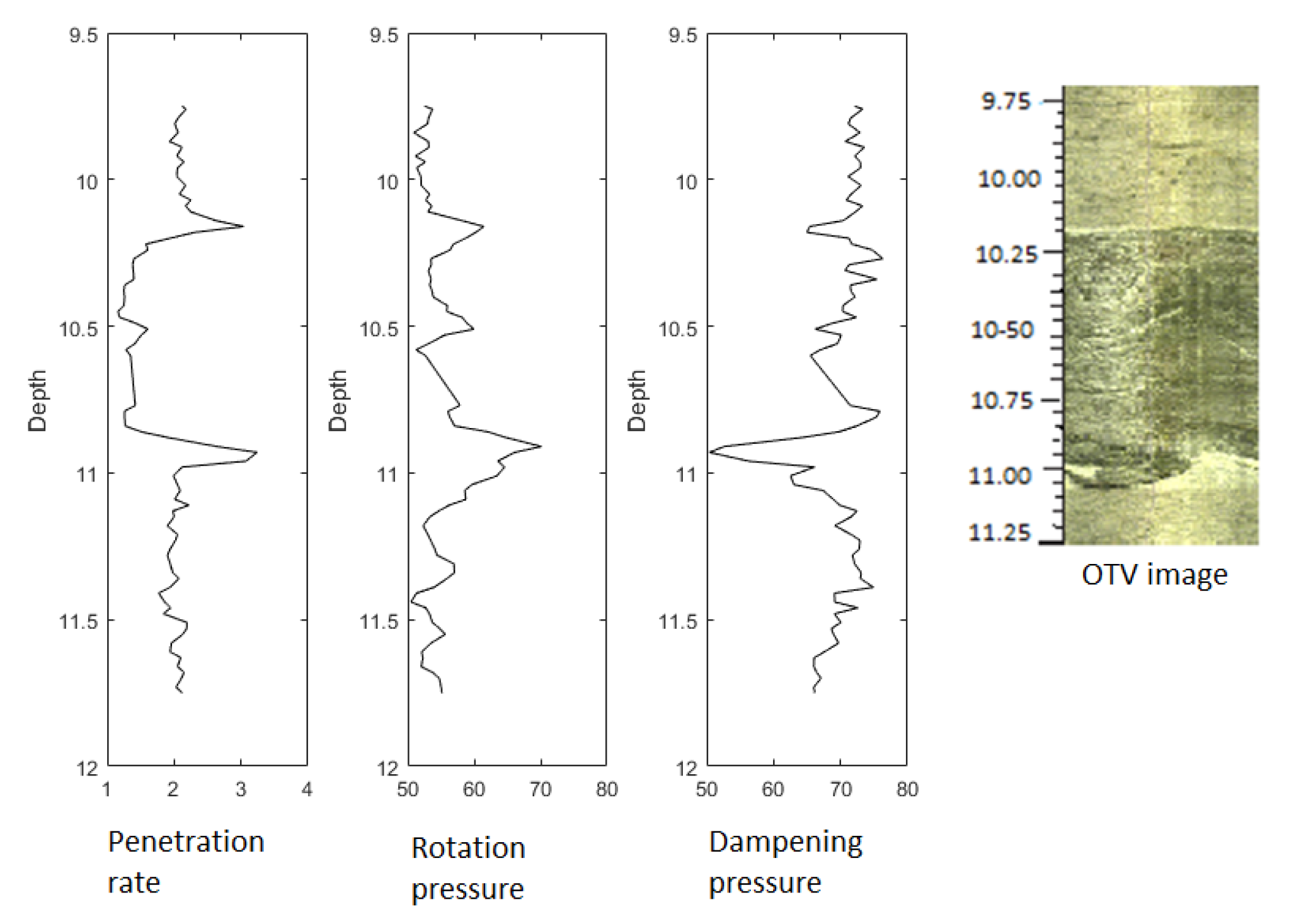
Figure 2 shows a zoomed OTV image of the intrusion in one of the boreholes at depth 10–11 m along with corresponding penetration rate, rotation- and dampening pressure. From this figure, one can see a strong relationship between the intrusion and the penetration rate, which is clearly lower inside the intrusion. Rotation pressure and dampening pressure are not as sensitive to this particular change in rock type, but both pressures show peaks at the beginning and at the end of this presumed intrusion.
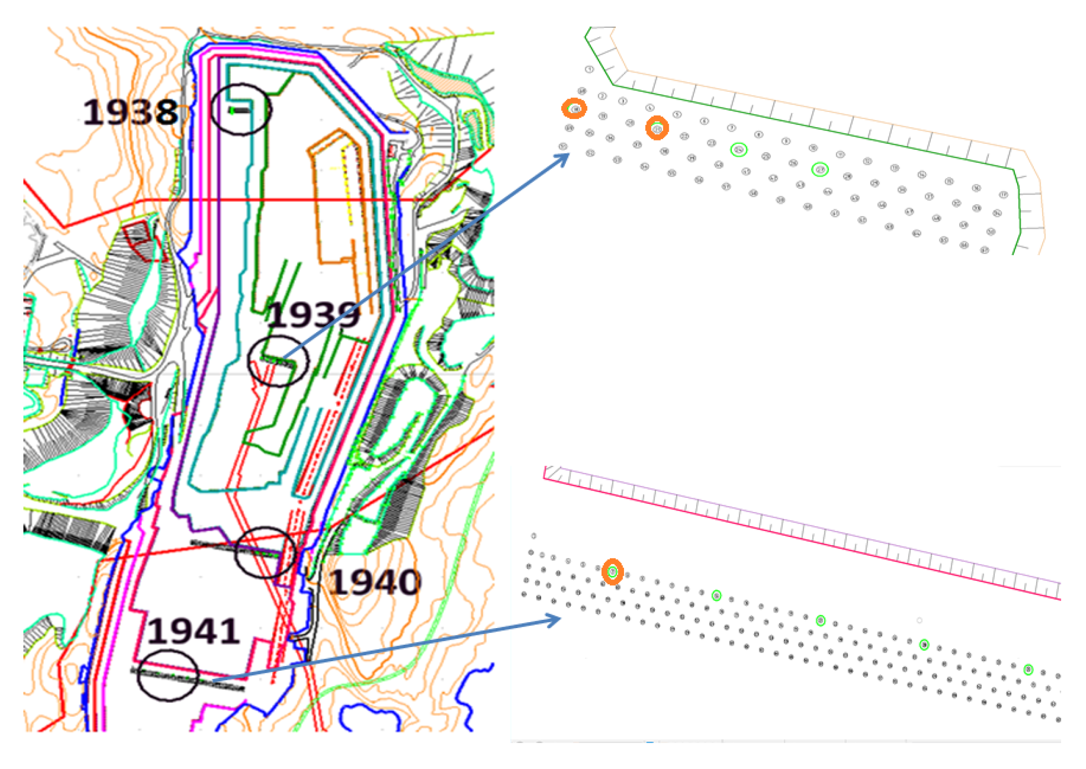
Data from borehole 1939-18, borehole 1939-21 and borehole 1941-7 are considered. The original MWD data from the selected boreholes are provided in the supplementary folder as Tables S1, S2 and S3 respectively. The boreholes are named with the blast number followed by a running number. Figure 3 shows the location map of the selected boreholes and blast numbers in the pit. The reasons for selecting these boreholes are based on the geological understanding of this area. Boreholes 1939-21 and 1939-18 are from the same blast 1939 and they are approximately only 3 m away. Therefore one would expect similar lithologies and fracturing patterns in these boreholes. According to the prior knowledge from the mine, blast 1939 contains intrusions of diabase or aplite which lower the overall quality of the blast. Borehole 1941-7 is from blast 1941, which is located in a different area. Instead of wide intrusions, small layers of banded, impure marbles and fractures are expected in this borehole.
Figure 4 shows the OTV images 1939-18, 1939-21 and 1941-7 respectively from left to right. High resolution images of the same boreholes are found in supplementary folder as Figures S1, S2 and S3 respectively. Along with the images, we also display a simpler numerical representation of the OTV image for every depth (black curves). The pixel values of the image are obtained using an image processing tool in Matlab (imread) and an average of pixel values at every depth is used for this numerical representation of OTV image. The image from borehole 1939-21 appears most homogeneous except for one or two clear wide intrusions (10–11 m and near 12 m). Borehole 1939-18 does not have such wide intrusions, but the one near 10 m is likely the same as one at similar depth in borehole 1939-21. Borehole 1941-7 has many variations and potential fractures that can be seen on the top and middle parts of the borehole.
3.2. Pre-Processing MWD Data
The original data from the rig will normally contain anomalies that occur due to both normal and abnormal operating conditions and mechanical error. To use the data for further analysis and to identify patterns, it is necessary to remove these anomalies from the raw data.
It is important to understand the drilling procedure to eliminate the unwanted data. At Brønnøy Kalk, drilling is done either manually or automatically depending on the operators and drilling conditions. The drilling operations are done in constant feed pressure settings in 2 different levels, low and high. Usually, the fragmented rock is drilled in a low-pressure setting in the rig. All data from upper part of the borehole were removed because this part of the rock is fragmented due to the blasting of the previous bench. After drilling through the fragmented part, the operator increases the pressure as part of standard procedure. A change point analysis using R package changepoint [15] on percussion pressure can detect the boundary between the pressure change [10], and the low-pressure parts are removed from further analysis. During drilling, a new drilling rod is attached on top of the previous one every 3.5 m. Feed pressure is the pressure that pushes the entire hammer downwards while drilling. During the time of rod change, this pressure will decrease considerably. After the rod change, the feed pressure increases gradually to the average. Data collected during the rod changes is not related to any mechanical properties of the rock. It is common to remove outliers by using 3 standard deviations and therefore, the data where feed pressure was less than three standard deviations away from its mean were removed from further analysis.
The processed data have unequal intervals in depth and also some data are eliminated during preprocessing. So a linear interpolation method is used [16] to assign data at equally spaced intervals at every 1 cm depth in the boreholes.
3.3. Hidden Markov Models
In this research, HMM are used to classify rock types from MWD data. HMM are popular for classification of discrete variables from indirect data. Reference [17] provides a recent overview of theory and several applications. References [18,19,20] demonstrate applications of HMM to borehole data of petrophysical variables collected to understand rock type alternation styles in the context of exploring for oil and gas resources. There are of course several alternatives to HMM for predicting the hardness variations of rocks from borehole data. Reference [21] use machine learning techniques such as boosting and neural networks on MWD data to study the lithological variations of the rock. Reference [22] study the drilling penetration rate for different drilling bits and rock formations using multiple regression models. An advantage of using HMM is the discrete sample space that naturally leads to classification and eases interpretation. The modeling assumptions of the HMM are outlined in the following sections, along with methods for predicting the hidden rock classes, and for parameter estimation. A summary of the implemented workflow for classifying rock types from MWD data is provided at the end of the section.
After the preprocessing, the MWD data are available at every 1 cm depth interval in the borehole. Data at a single depth index are , where , , is one of the MWD measurements described in Section 3.1, say penetration rate, and m is the number of measured variables. In the presentation it is assumed that m is the same for all depths, but a sensitivity study to the size and configuration of different MWD data variables is conducted in the results section. For instance, it is interesting to understand which of the MWD variables discussed in Section 3.1 are more important for marble classification. The vector of all measurements, from the start of the borehole to depth index i, is denoted . This collection of data will be important for the subsequent analysis, since the approach considered here will integrate the data recursively, including one more MWD depth index at a time. This means that the methodology implicitly incorporates a down-the-hole spatial correlation between MWD data points. At the deepest index considered, all data are included. The analysis is performed from top to bottom because this is the way drilling data are acquired. An alternative, is to let the Markov transition mechanism mimic geological deposition over time.
At a single depth index , denotes the marble rock class. In this case study, rock classes {a priori pure marble, fractured rock, intrusion}, will be used. The vector of marble classes is denoted . As stated in the introduction, the main goal of this paper is to use and present the HMM approach for classifying these rock classes at all depths effectively from the MWD data.
HMM are based on a Markov chain model for the rock classes . A first order Markov chain is considered. The Markov property means that the conditional probabilities are
which means the rock type at each depth depends only on the rock type at the previous depth. Importantly, the variable is dependent on , but when is known, the variables and are independent.
It is common to assume that the probabilities in Equation (1) are constant within the depth domain of interest, i.e., . The Markov chain is then said to be time-homogeneous. The probabilities can be organized in a transition matrix , where the rows correspond to the current state , while the columns correspond to the next state , . For , the transition matrix is
Because of the discrete state space model, each row in the transition matrix must sum to 1, so , for all .
The initial probabilities are denoted by , , where . The joint model formulation for the rock classes along the entire borehole length is then
Equation (3) provides a framework for simulating a Markov chain. An algorithm for stochastic simulation from the model would start at the top index, and sample a class from discrete probability vector . Next, the program would move recursively through the indexes , sampling from the correct row in the transition matrix, i.e., , when the sampled rock class k is given at the current depth index. Figure 5 shows realizations from two different Markov chain models each of length . The two transition matrices are
In the left display, the classes either stay the same or move one class up (except from class 3, where the chain moves to 1).
This might be natural for some geological deposits, where there has been fining or coarsening sequences over time, giving these kinds of alternation styles. In the right display, there is less ordering in the alternation and less continuity in the sense that the rock classes change more often.
The MWD data at a depth index is dependent on the rock class at that depth. For instance, the penetration rate can be smaller in hard rock intrusion than in the pure softer marble. In HMM this dependence between the rock class and the various MWD data is modeled by a likelihood model. Here a likelihood is defined for all depth indexes considered. Here, is the expected value of MWD data when the marble rock class is k, and is the measurement error covariance matrix, which is assumed to be the same for all rock classes. This covariance matrix of the measurements is of size ;
where is the variance of MWD measurement (e.g., rotation pressure) and is the covariance between MWD measurement and (e.g., rotation pressure and penetration rate).
Figure 6 shows an illustration of two different likelihood models.
Here, there are bivariate MWD data, with data variable 1 on the first axis and data variable 2 on the second axis. There are three rock classes in this illustration (d = 3), and their likelihood models are indicated by the three ellipse shapes, representing Gaussian probability contours, and 25 data points from the three classes (plotted as plus, circle and diamond). In the left display it is difficult to separate the three classes. In the right display the means are more separated, and it would be easier to classify the rock classes from a data variable .
Note that the likelihood model is defined for each location, and dependence only on the rock class at the particular depth at which the MWD data are measured. Statistically this means
Just like for the Markov property in Equation (1) this likelihood model formulation states conditional independence assumptions. The data will be dependent on , and it will also be dependent on , but once is known, the data variable is conditionally independent of the remaining variables.
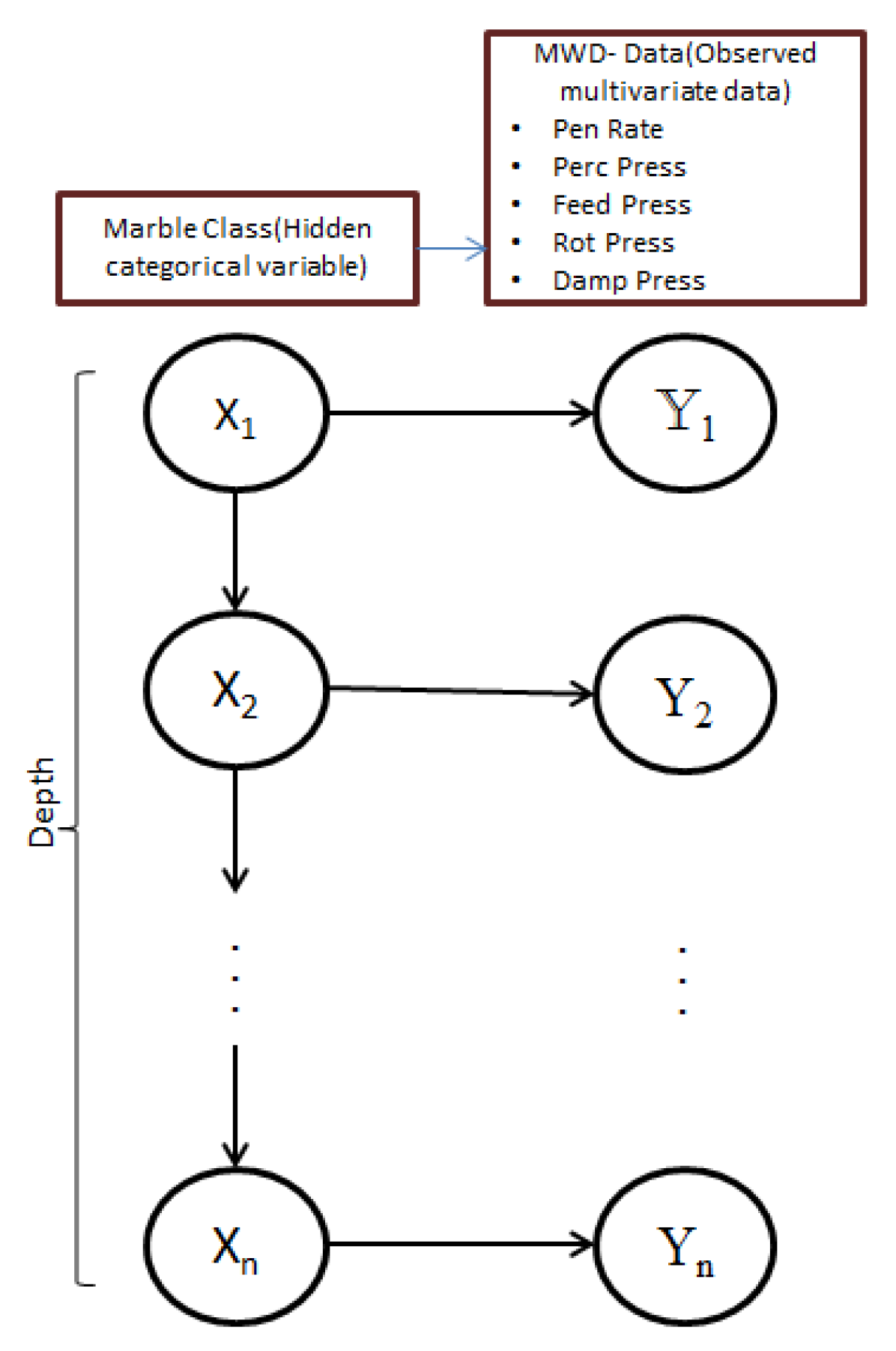
Figure 7 gives an illustrative summary of HMM for MWD classification. The dependencies involved in the modeling are illustrated by the Markov chain model with edges going downwards to the left, and with edges for the conditional independent likelihood model pointing from left to right.
The goals associated with HMM are to find
- Most likely sequence of rock classes given all MWD data: .
- Estimation of model parameters , , for , and .
The key steps for solving these tasks are provided next. For more background, see Appendix A or e.g., [23].
3.4. Rock Class Prediction
One can classify the rock class from data at every depth , using the joint conditional probabilities . The classification requires the computation of conditional probabilities. These are computed by sequentially going through the indexes, and in doing so conditioning on the data. The sequential routine is possible because of the Markovian structure and conditionally independent data, where it is sufficient to regard only two variables at a time. This method is sometimes called the forward-backward algorithm which is explained in Appendix A.
The most likely joint combination, or maximum a posteriori (MAP), of rock classes can be found by the Viterbi algorithm which solves
The Viterbi algorithm obtains the solution to Equation (5) by a forward-backward evaluation and a maximization part. Starting at the last index n
For subsequent maximization is used as follows:
The required probabilities are further explained in Appendix A.
3.5. Parameter Estimation—EM Algorithm
The expressions for the Viterbi solution in Equation (5) require specification of the model parameters. These can be estimated using an iterative approach called the Expectation Maximization (EM) algorithm. In the current setting the parameters are the transition matrix for marble rock class , the initial vector , the mean in the likelihood , , and the likelihood model covariance matrix .
Initially, one must assign some values to the above mentioned model parameters. The EM algorithm uses a combination of probability calculation and optimization to assess parameter values. (See Appendix B for details.)
In the E-step, based on the current set of model parameters and the data, one calculates the marginal probabilities and . In the M-step, the model parameters , , and are updated using the probabilities found in the E-step.
3.6. Workflow Summary
The entire workflow of the EM algorithm and the prediction is given in Algorithm 1.
| Algorithm 1 Workflow. |
|
Convergence of model parameters is monitored by looking at the change in parameter values at every iteration. When this is very small, the algorithm stops. The current parameters are then said to be maximum likelihood estimates. They are plugged into the classification algorithm described in Section 3.4.
A priori, three rock classes in each borehole is assumed based on knowledge about the deposit; namely intrusions (e.g., diabase and aplite), marble and fractured zones. To identify the model that best predicts the rock classes, assuming , different combinations of MWD data are studied. The MAP predictors of the tested models are compared with the OTV image and the other logging data to recognize the information-content of MWD data variables. Initially, borehole 1939-21 is selected for analysis because this borehole shows a very clear intrusion in the OTV-image and it was presumed easier to visually compare the MAPs with the OTV image from this borehole compared to the others. Next, two other boreholes are analyzed using the same technique.
The main R codes and Matlab codes used in this study are provided together with a readme-file as supplementary information.
4. Results
The means and standard deviations of MWD data in the different boreholes used in this study are shown in Table 1.
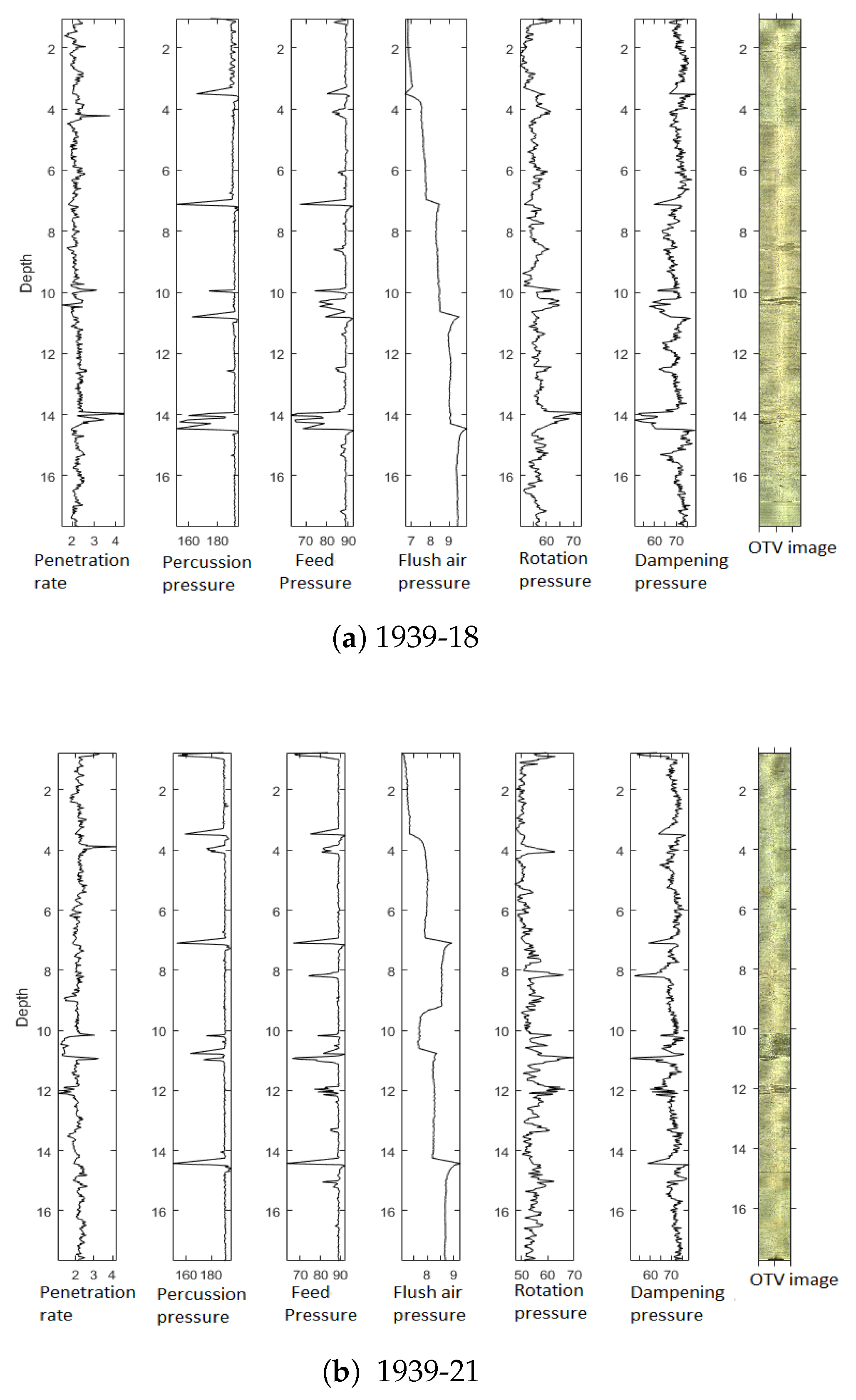
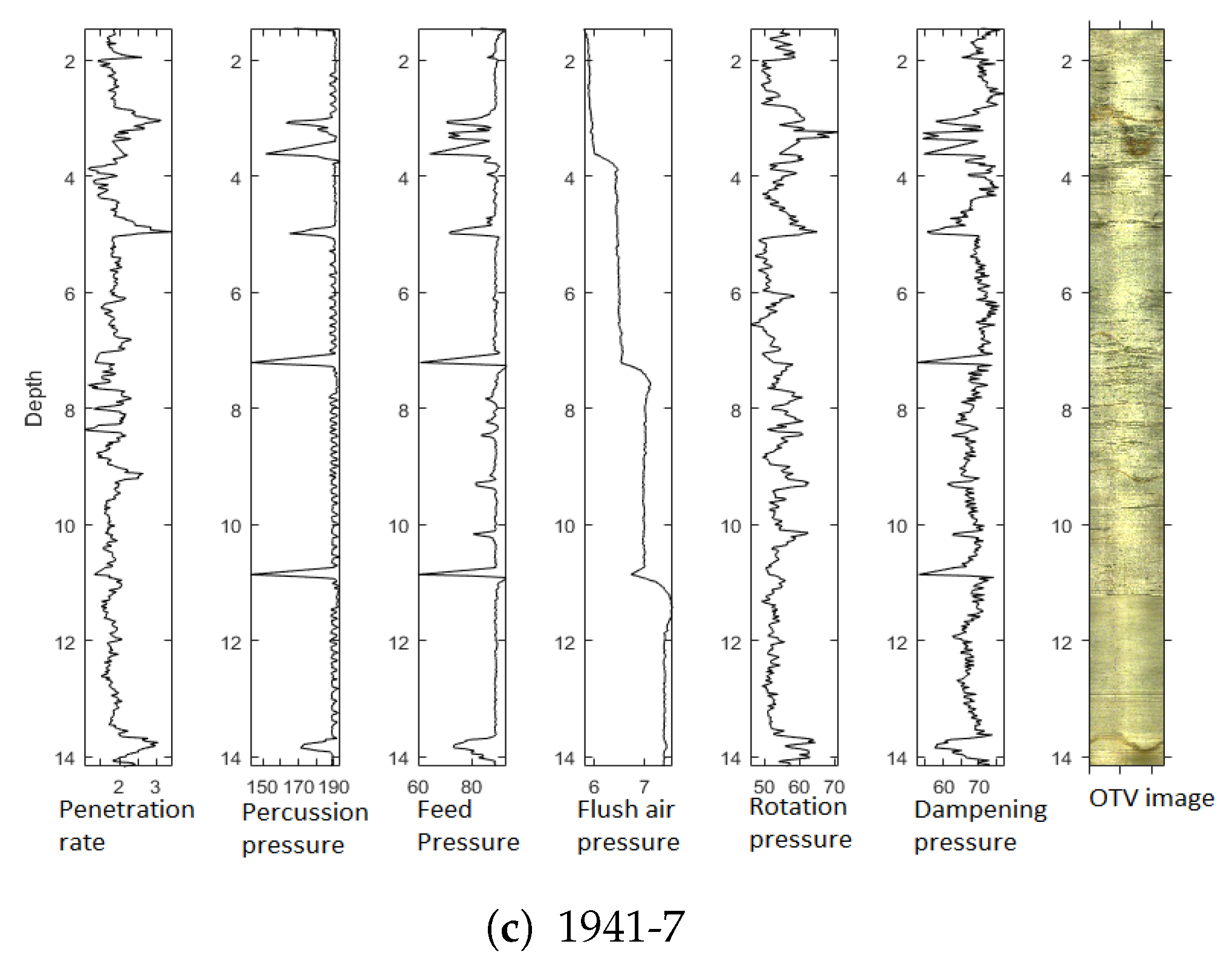
The cleaned MWD data and the corresponding OTV image of the boreholes 1939-18, 1939-21 and 1941-7 are illustrated in Figure 8.
4.1. Identifying the Best HMM for Rock Classification
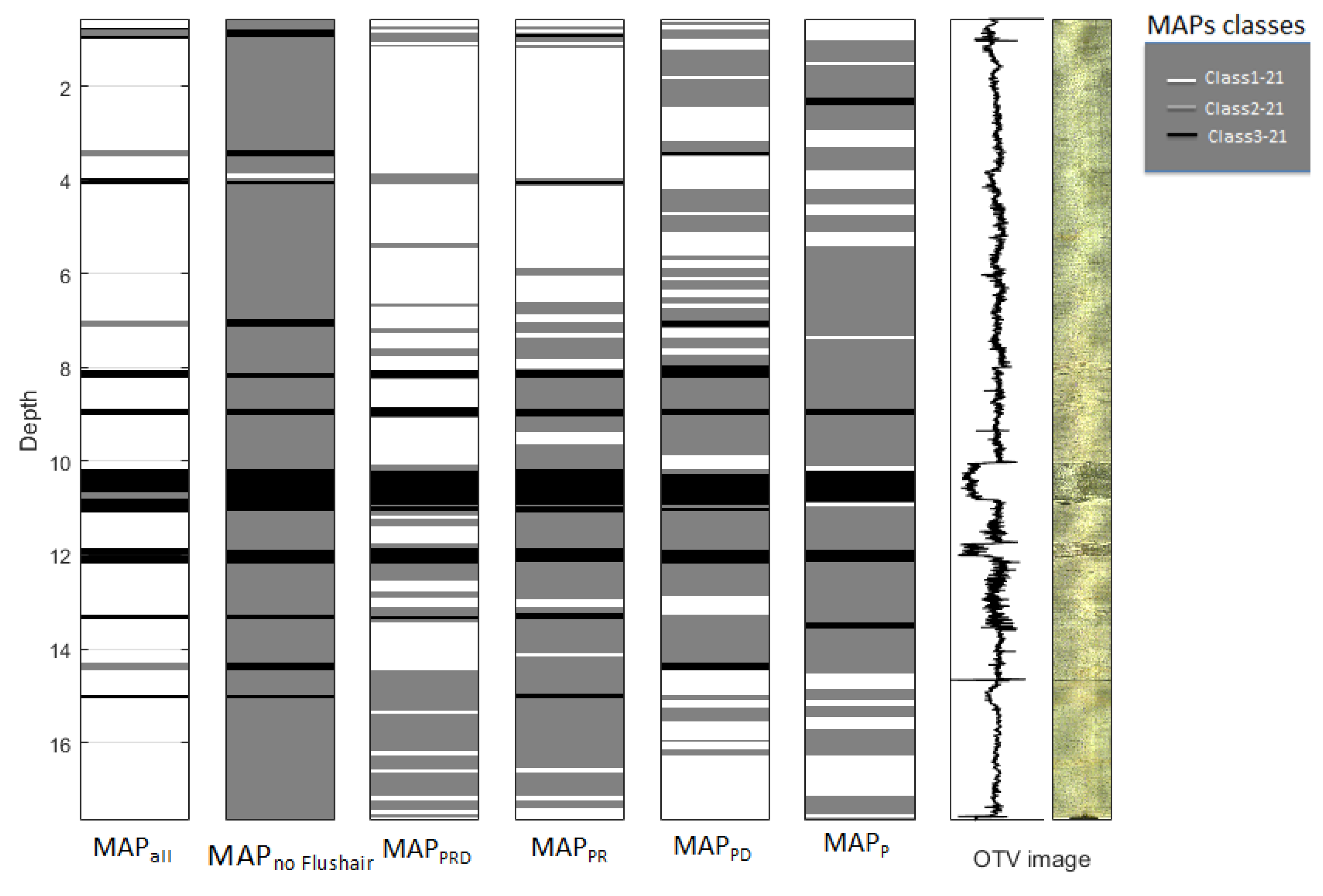
MAPs of some of the tested models and the OTV image of borehole 1939-21 are displayed in Figure 9. The three different rock classes predicted at a particular depth using MAP are shown by different colors (white, grey, black). As the classes are created for each borehole, they are named with a class number followed by its borehole running number. For example, class1-21, class2-21, and class3-21 refer to the three classes in 1939-21. The initial two MAPs from left in Figure 9 are using the model with all MWD data (MAPall) and the model with excluding flush air pressure (MAPNoflushair). The third one is using penetration rate, rotation pressure and dampening pressure (MAPPRD), the fourth is using penetration rate and rotation pressure (MAPPR), the fifth is using penetration rate and dampening pressure (MAPPD) and the final one is using only penetration rate (MAPP).
Figure 9 suggests that among the tested MAPs, all of them are able to identify the two main intrusions at depth 10–11 m and at 12 m that are seen in the OTV image of that borehole. However we eliminated some models from further analysis because of following reasons.
- Even though fluctuations due to rod change are eliminated in the pre-processing, feed pressure and percussion pressure are showing trends in approximately every 3.5 m depth (see Figure 8). This variation is also visible in dampening pressure with less intensity. In Figure 9, one can see that MAPall, MAPno Flushair and MAPPD are showing trends in approximately every 3.5 m depth. Because of this possible mis-classification we are not considering MAPall, MAPno Flushair and MAPPD for further analysis.
- The penetration rate depends on the pressures and the rock characteristics. In theory, a model with more variables will give better results. So MAPP is also not considering further.
As a result, two MAPs; MAPPR and MAPPRD are selected for further analysis. TGAM (cps), K (%), U (ppm), Th (ppm), MSUS, MAPPRD and MAPPR along with a zoomed OTV image of the borehole 1939-21 are displayed in Figure 10. Class3-21 in MAPPR and MAPPRD are compared with peaks in TGAM, MSUS and a zoomed OTV image of the borehole. The result shows that MAPPRD is better at classifying all the visible peaks in MSUS and SGAM as class3-21.
The same selected MWD data has also been applied to other boreholes and the MAP predictions are compared with logging data. The HMM using penetration rate, rotation pressure and dampening pressure is applied to boreholes 1939-18 and 1941-7 MWD data, and the corresponding MAPs are displayed in Figure 11 for borehole 1939-18 and Figure 12 for borehole 1941-7. In the figures, on left, depth plots of TGAM (cps), K (%), U (ppm), Th (ppm) and MSUS, are displayed. Adjacent to the logging data, the corresponding MAPPRD predictor is displayed. The OTV image along with its numerical representation of the image of the borehole can be seen in the rightmost displays.
4.2. Precision and Characteristics of Predicted Classes
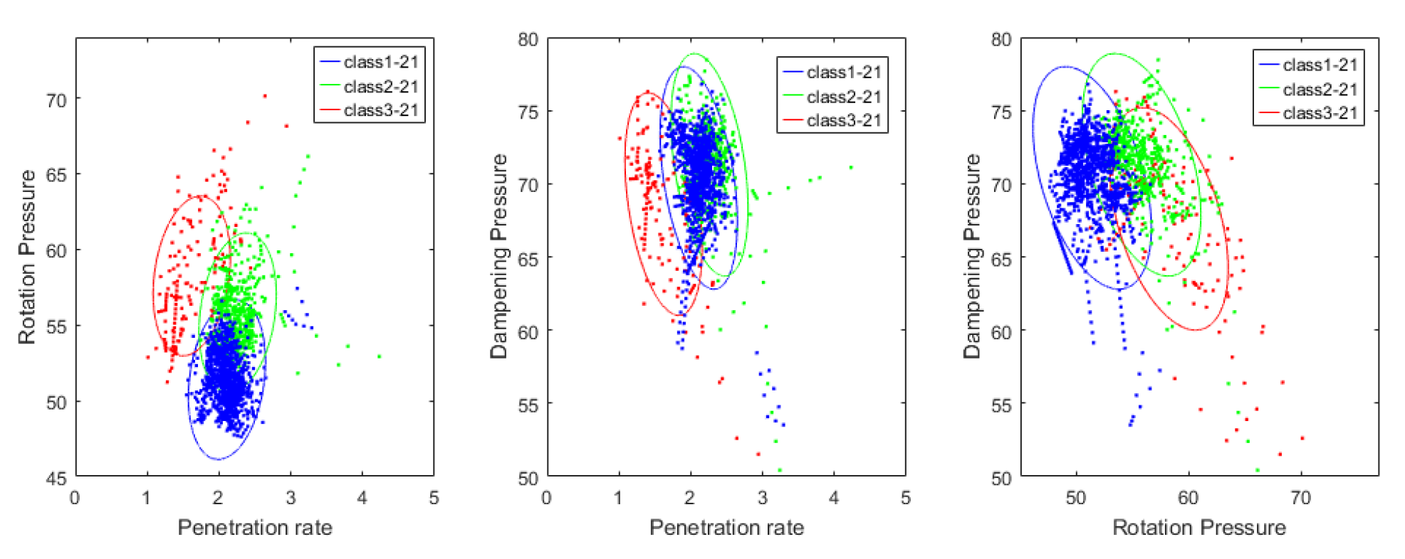
Figure 13, Figure 14 and Figure 15 show the scatter plots using all pairs of the selected data for borehole 1939-21, 1939-18 and 1941-7 respectively. In each of the figures from left, the first one is plotting penetration rate vs rotation pressure, the second is plotting penetration rate vs dampening pressure and the third one is plotting rotation vs pressure and dampening pressure. The three ellipse contours in each scatter plot are created using the corresponding Gaussian likelihood model parameters of three classes estimated by EM algorithm for each borehole. The colors in the scatter plots and the ellipses represent the classes assigned to each point according to corresponding borehole’s MAPPRD.
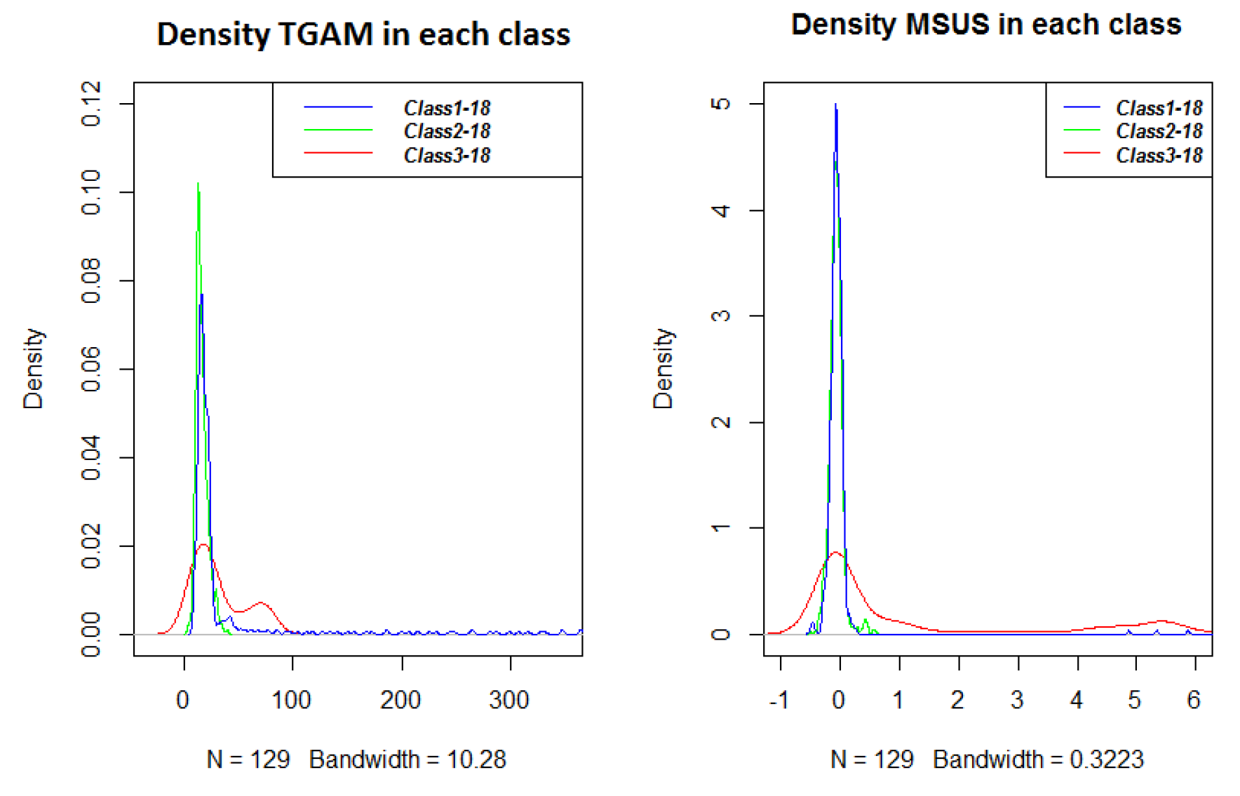
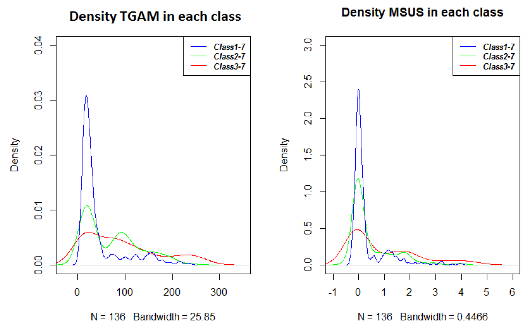
In Figure 16, Figure 17 and Figure 18 the density plots of TGAM (left) and MSUS (right) are plotted using the data respectively from borehole 1939-21, 1939-18 and 1941-7. The three classes of MAPPRD are used to select the subsets of the data. And this is done in every borehole. The color code in the densities match with ellipses and scatter plot in Figure 13, Figure 14 and Figure 15.
The different rock classes can be characterized by the average penetration rate, rotation pressure and dampening pressure. Table 2 shows the summary statistics within each class. The last column of the table shows the assigned characteristic of the classes when compared with OTV image and other logging data.
5. Discussion
The lithologies penetrated by boreholes at different locations will have different rock strengths and characteristics, and these differences in rock strength and structure will affect the MWD data pattern. From Table 1 we can see that borehole 1941-7 on average has a lower penetration rate and a high standard deviation. This is partly due to the fact that it has a lower rotation and dampening pressures. Usually, with more fracturing and heterogeneous rock characteristics, one may encounter instability while drilling. Such unstable drilling conditions may lower the penetration rate. Percussion pressures are on average similar, with a slightly elevated standard deviation in borehole 1941-7. This applies to feeding pressure as well. Flush air pressure is lower in 1941-7. This again indicating that there are some fractures which does not need much pressure to flush out as the density of rock material is less inside fractures or cracks. Rotation pressure is highest in borehole 1939-18 and lowest in 1939-21. The standard deviation is highest in 1941-7, possibly because of more fractures. Borehole 1939-21 has the highest average dampening pressure, whereas the lowest value can be found in hole 1941-7.
The estimated likelihood model of the selected HMM and the density of the logging data inside every class are used to identify the properties of the locally created classes in each borehole. In Figure 10, the big peak in MSUS and a small peak in TGAM are visible at depths around 10 m and 12 m. The high MSUS suggests that the section of the borehole probably contains diabase, and this area is classified as class3-21. Around depth 8–9 m, there are two peaks only in TGAM which indicates that the lithology at this depth is a different lithology than the intrusion mentioned above at depth 10 m and 12 m. The high level of SGAM shows that this section probably contains more potassium and thus indicating aplite. This is clear from the vertical profile of K in the same display. Note that there is a scale difference between K and U and Th as K is given in percentage. When comparing with the OTV image, one can see that this intrusion is not very prominent in the picture, still the MAP has classified this area as class3-21.
According to the first and second scatter plots in Figure 13, the penetration rate is clearly lower in class3-21 compared to other two classes. One can see a clear separate cluster in both scatter plots in which penetration rate is involved. Also class3-21 has higher rotation pressure and lower penetration rate. This implies that rock type in class3-21 is harder and has clearly different rock characteristics compared with the other two groups. Moreover, Figure 16 suggests that most of the radioactive- and magnetic material belong to class3-21. The distribution of MSUS has a very high standard deviation because the aplite is not magnetic, but it is still an intrusion and classified as class3-21. This shows that class3-21 in the HMM classification is having more impure materials than class1-21 and class2-21 and this group represents an intrusion class.
Note that 1939-18 is located near the initial borehole 1939-21. So we expect similar rocks in these two boreholes. The two small intrusions in 1939-18, are possibly the same intrusions as in borehole 1939-21, at depths near 8 m and 10 m, as seen in both the classification results and the OTV image (See Figure 10 and Figure 11). Similar to 1939-21, a big peak in MSUS and a small peak in TGAM around 10 m depth and a big peak in TGAM around 8–9 m depth are visible in borehole 1939-18. This suggests that they are the same intrusion layer, but in 1939-18 they are smaller in thickness. In the MAP results, the MSUS peak is clearly classified as class3-18, but the area of the peak in TGAM at depth 8–9 m is not completely classified as class3-18 in the MAP. Moreover, in the MAP of 1939-18, one can see more areas predicted as class3-18 but there is no visible change in MSUS or TGAM. For example, at around depth 14m, an area of about 0.5m thickness is classified as class3-18. There is no visible change in TGAM and MSUS in that area, but a clear color change in OTV image in that section can be seen. There are also very clear peaks in penetration rate, rotation pressure and dampening pressure visible in that area. The contradictory data are probably due to fractures.
Unlike in class3-21, Figure 14 shows that class3-18 has the highest mean rotation pressure and highest mean penetration rate. So one cannot clearly say that the marble inside class3-18 is a harder rock intrusion. But the class3-18 is very well separated from other classes in the two scatter plots and the ellipses that involve the dampening pressure. This suggests that class3-18 is different from class1-18 and class2-18. Class3-21 and class3-18 have also different MWD characteristics. Class3-18 is suggestively a combined class of both intrusion and some fracturing of the marble deposit. Also, class3-18 intrusions are much smaller in thickness and the MWD data inside these intrusions act like fractures because the drilling procedure is fast. As soon as the rig increases its pressure to drill through the hard intrusion, the hard part will end. So the pressure increase helps to increase the penetration rate. Figure 17 indicates that most of the impure marble classified as class3-18 and marble that have no contents of MSUS or TGAM is classified as class3-18 as well. Also, it can be seen that class1-18 and class2-18 are pure marble and most of the impure marble which contain the magnetic and radioactive minerals belong to class3-18.
In Figure 13 the scatter plots and the ellipses of class1-21 and class2-21 are not well separated and similarly in Figure 14 for class1-18 and class2-18. This indicates that these two classes are not actually different in both boreholes. As the number of classes is pre-selected in the modeling, it will give three different classes even though the actual difference between the classes are small. Here, a slight increase in penetration rate in class2-18 and class2-21 compared to class1-18 and class1-21 is seen due to a slight increase in rotation pressure. This can probably be due to a smooth drilling process. Figure 16 and Figure 17 also suggest that the distribution of magnetic rock and radioactive material is similarly distributed and comparatively lower for class1-18, class2-18, class1-21, and class2-21.
Borehole 1941-7 is expected to behave differently than the other boreholes. According to Table 1 average penetration rate is lower than in the other boreholes even though the average rotation pressure is not low. The standard deviation of penetration and rotation is also higher in 1941-7 compared to the other two boreholes. There is no wide clear intrusion, but there are several small and frequent changes, possibly small intrusions and fractures are visible in the OTV image. This applies especially to top, middle and very bottom part. After 10 m depth, the borehole is homogeneous in color until it reaches depths of more than 13m. Borehole 1941-7 is expected from the general geological understanding of the deposit to be more heterogeneous than 1939-21 and 1939-18. MAPs with OTV image and other logging data in Figure 12 show that the top and middle part of the borehole is having more class changes. In this area, the OTV image colors are very heterogeneous and MSUS and TGAM are very high.
In Figure 15, it can be seen that in first scatter plot using penetration rate and rotation pressure, the three classes are well separated. In the second and third scatter plots, class3-7 is a separate cluster. This indicates that for borehole 1941-7, class1-7, class2-7, and class3-7 are having fairly different characteristics. In Figure 12, one can see that the class3-7 coincide with the big variation on top of the borehole around 3m depth and some small variations in the middle of the borehole and a visible color difference in the OTV image at the bottom of the borehole. The bottom of the borehole is not having any signals in the MSUS and TGAM but still classified as class3-7. This indicates that this is not related to any impurities but possibly related to some fracturing or cracks. So class3-7 is mainly fractured marble and fractured impure marble zone. This means that class3-7 is having similar characteristics as class3-18.
Unlike in the other boreholes, we can see from Figure 12 that class2-7 also represents an impure marble class. Both MSUS, SGAM, and TGAM are high in both class2-7 and class3-7. Class2-7 is frequently visible in the middle and top of the borehole in that borehole’s MAP-PRD. So this class represents most of the impure marble except for the wide fracture zones inside impure marbles. Figure 18 shows that the distribution of SGAM and MSUS in all the classes in this borehole are different. Class2-7 and class3-7 are having significant amounts of magnetic and radioactive material and class1-7 is mainly consisting of pure marble. As discussed in Section 3.1, the area of blast 1941 is expected to have a mixture of pure, impure and banded marble. It is convincing to believe that the 3 classes have different rock characteristics.
Class3-21, class3-18, and class3-7 are characterized by a higher rotation pressure than the other rock classes of respective boreholes. The fractures and small intrusions representing class3-18 and class3-7, are also showing a comparatively lower dampening pressure than in thick intrusions. Class3-21 is a thick intrusion and have a lower penetration rate, but not much decrease in dampening pressure. This is making sense because dampening pressure acts as a pressure to make the rig stable while drilling. So while drilling fractures, it tries to adjust the pressure to make the drilling process smoother. Class2-7 and class3-7 are confirmed as impure according to the OTV-image and the other logging results. These two marble classes have higher mean rotation pressure than class1-7. Class1-7 is considered as a pure marble group because the distribution of MSUS and TGAM are similar to that of the pure marble classes in 1939-21 and 1939-18.
If the rock formation penetrated by a borehole is totally homogeneous the bi-variate Gaussian ellipse is expected to be very much interlinked and all the scatter plot clusters will be hard to separate. To penetrate through a hard rock type, a higher rotation pressure needs to be applied. Rotation pressure will also be high in broken and uneven fracture zones. Penetration rate will be low on hard intrusions, but high in fracture zones. MWD data inside very thin intrusions resemble MWD data from fracture zones. So the increase or decrease in rotation pressure is an indication of a change in rock type. Also, the high variation in dampening pressure between the classes indicates the class with lower dampening pressure has lots of fractures or small intrusions.
Based on the HMM-based analysis of the MWD data in three different boreholes, three to four different rock classes have been identified. These are pure marble, intrusions, fractured zone and impure marble. These have different MWD characteristics. See Table 2. Rock type “pure marble” would have a penetration rate of around 2 m/min, a rotation pressure around 51–54 bar, dampening pressure around 70–71 bar and a relatively low magnetic susceptibility and spectral/total gamma. This rock type can be represented by class 1 and class 2 from borehole 1939-18 and 1939-21. This marble group is having relatively average strength or hardness. Rock type “intrusion” is characterized by a low penetration rate, an on average high rotation pressure (but varying), an average dampening pressure around 69 and an extremely high magnetic susceptibility and spectral gamma. No division has been made between the type of intrusions, but the possible lithologies present in this case are diabase and aplite. So this class is harder than the “pure-marble” class. This rock type is represented by class3-21. Rock type “fractured marble” has a high penetration rate, a high rotation pressure, a low dampening pressure, a low magnetic susceptibility and a relatively high total gamma. This is due to impurities intervened with the fractures. Fractured marble is represented by class3-18 and class3-7. The fractured marble is softer rock zone than other rock classes. Rock type “impure marble” is represented by class1-7 and class2-7 and is characterized by a low penetration rate, a low to medium rotation pressure, a relatively high dampening pressure and a low magnetic susceptibility and a relatively high total gamma. The impure marble zone is relatively harder than pure marble suggestively due to the presence of thin impurity intrusions of diabase or aplite. Given these rock types and their characteristics, the rock material penetrated by the boreholes can be classified and used in the development of a 3D-model of in-situ rock type variations. However, this model will be tested on more boreholes in different locations of the mine before it is used in further development. We aim to report the results of more advanced modeling and testing in future work.
Geological data are to a varying degree always spatially correlated. Normally, the spatial correlation is quantified through the variogram. The methodology implemented here resembles to some extent a traditional cluster analysis. A cluster analysis will also classify data points based on some distance measure, but a cluster analysis will not take spatial correlations into account. Spatial correlation is in the HMM taken implicitly into account through the transition probability. This makes the implementation of HMM superior to the traditional implementation of the cluster analysis.
The mining company is annually drilling approximately 2000 boreholes. MWD data are collected on average every second centimeter. Huge amounts of data are thereby collected. Manual interpretation of such amounts of data including a rock type classification is not manageable. It is decisive to have routines and tools that automatically can classify rock types. Potentially this will enable the development of a high-resolution geological model that in the future may be incorporated in mine planning and reconciliation. This is also of uttermost importance in an geometallurgical context. Geometallurgy is about linking in-situ geological properties with processing or metallurgical performance. This performance is normally measured by KPIs. Knowing the rock classes in a blast will render it possible to assess the processing performance of this blast. This places the analysis of MWD data and the utilization of the results in the planning process into the core of geometallurgy.
6. Conclusions
A new method to classify rock types according to its rock strength and hardness, especially hard rock intrusions in a marble deposit, using MWD data collected during normal bench drilling is proposed. A statistical hidden Markov model is used to describe rock classes and data, and the Expectation Maximization algorithm is used to specify the parameter in this model. By applying these methods on different combination of MWD data, it can be concluded that penetration rate, rotation pressure and dampening pressure together can identify and classify hard intrusions, fractured zones and marble inside a borehole. The MWD data behave differently inside thick intrusions and very thin intrusion. Thin intrusions and fractures have similar MWD behavior. One has to consider the fact that during the actual mining procedure the logging data (the OTV-image, the magnetic susceptibility and the spectral- and total gamma) will not be available. By comparing new MWD-data and the characteristics of the MAP-classes defined in this research, it would be possible to assign a class to every data point. A priori knowledge about the lithological variations is helpful to choose the number of classes in advance. Cross-plotting of the bi-variate model fit of data is a helpful visualization tool and provide a valuable aid in interpreting the classes. The results presented in this paper might be used to develop an index quantifying the blast heterogeneity. In future research, this will be used to develop an improved sampling strategy.
Supplementary Materials
The following are available at https://www.mdpi.com/2075-163X/8/9/384/s1. Table S1: MWD data for borehole 1939-18, Table S2: MWD data for borehole 1939-21, Table S3: MWD data for borehole 1941-7. Figure S1: High resolution OTV image of Borehole 1939-18, Figure S2: High resolution OTV image of Borehole 1939-21, Figure S3: High resolution OTV image of Borehole 1941-7. The main MATLAB codes and R code are also be found in the folder. A “Read me” is also available, which will help to properly run the codes.
Author Contributions
Three authors have their valuable contributions in this article. Conceptualization, V.V. and J.E.; Methodology, J.E.; Software, J.E. and V.V.; Validation, V.V.; Formal Analysis, V.V.; Investigation, V.V. and S.E.; Resources, S.E. and Veena.Vezhapparambu; Data Curation, V.V.; Writing—Original Draft Preparation, V.V.; Writing—Review & Editing, S.E. and J.E.; Visualization, V.V.; Supervision, J.E. and S.E.; Project Administration, S.E.; Funding Acquisition, S.E.
Funding
This work is a part of Ph.D. program of the author Veena Vezhapparambu. The work is funded by the Norwegian Research Council and industry partners, Brønnøy Kalk AS, Verdals Kalk AS and Sibelco Nordic AS, through InRec (Increased Recovery in the Norwegian Mining Industry by Implementing the Geometallurgical Concept) project with project number 10432900.
Acknowledgments
The authors acknowledge Brønnøykalk AS for the data support. We also would like to thank Håkan Schunnesson for his valuable suggestions and Dirk van Oosterhout for his help during the logging data collection and logging image processing.
Conflicts of Interest
The authors declare no conflict of interest.
Abbreviations
The following abbreviations are used in this manuscript:
| MWD | Measurement while drilling |
| HMM | Hidden Markov Models |
| MSUS | Magnetic Susceptibility |
| SGAM | Spectral gamma |
Appendix A. Forward-Backward Algorithm
The forward recursion computes the filtering probabilities and the one-step prediction probabilities .
The filtering probabilities for are given by
where the starting point is . The prediction is obtained by
where we marginalize out the rock class at depth index i. Note how the Markovian structure and the conditional independence assumptions for data simplify in the conditioning.
The backward recursion starts at the last filtering probability, , and then it steps backwards recursively. The backward equation is
where the first right-hand side probability in Equation (A3) is
Appendix B. Parameter Updates in EM Algorithm
The probabilities and , , , are computed by the forward-backward algorithm, using the current parameter values. This is the E-step of the EM algorithm. In the M-step, the parameters are updated using these probabilities and the data. The formulas for updating are given next.
First, for the initial probabilities;
The transition probabilities are
With regard to the likelihood parameters, each class, i.e., and for each MWD parameter , the mean is
which is an average over the data, weighted by the probabilities. If we consider MWD variables ’Penetration Rate’ and ’Rotation Pressure’, and classify the borehole as 3 categories of rocks, then d will be 3 and m will be 2. The likelihood covariance matrix is estimated by
References
- Lamberg, P.; Rosenkranz, J.; Wanhainen, C.; Lund, C.; Minz, F.; Mwanga, A.; Parian, M. Building a geometallurgical model in iron ores using a mineralogical approach with liberation data. In Proceedings of the The Second AUSIMM International Geometallurgy Conference, Brisbane, Australia, 26 November 2013; Volume 30, pp. 317–324. [Google Scholar]
- Bunkholt, I. Beneficiation of Carbonates—Interactions Between Raw Material Properties and Processing Performance to High-Grade Fluid Filler and Coating for the Paper Industry. In Minerals Engineering; Luleå Technical University: Luleå, Sweden, 2011. [Google Scholar]
- Watne, T. Geological Variation in Marble Deposits: Implication for the Mining of Raw Material for Ground Calcium Carbonate Slurry Products. Ph.D. Thesis, NTNU Trondheim, Trondheim, Norway, 2001. [Google Scholar]
- Marinos, P.; Hoek, E. Estimating the geotechnical properties of heterogeneous rock masses such as flysch. Bull. Eng. Geol. Environ. 2001, 60, 85–92. [Google Scholar] [CrossRef]
- Xie, H.; Pei, J.; Zuo, J.; Zhang, R. Investigation of mechanical properties of fractured marbles by uniaxial compression tests. J. Rock Mech. Geotech. Eng. 2011, 3, 302–313. [Google Scholar] [CrossRef]
- Vezhapparambu, V.S. Increased geometallurgical performance in industrial mineral operations through multivariate analysis of MWD-data. Tech. Note Mineralproduksjon 2016, 7, B25–B32. [Google Scholar]
- Rai, P.; Schunesson, H.; Lindqvist, P.A.; Kumar, U. An Overview on Measurement-While-Drilling Technique and its Scope in Excavation Industry. J. Inst. Eng. Ser. D 2015, 96, 57–66. [Google Scholar] [CrossRef]
- Ghosh, R.; Schunnesson, H.; Kumar, U. The use of specific energy in rotary drilling: The effect of operational parameters. In Proceedings of the International Symposium on the Application of Computers and Operations Research in the Mineral Industry, Fairbanks, AK, USA, 23–27 May 2015. [Google Scholar]
- Segui, J.; Higgins, M. Blast design using measurement while drilling parameters. Fragblast 2002, 6, 287–299. [Google Scholar] [CrossRef]
- Vezhapparambu, V.S.; Ellefmo, S.L. Change point analysis of MWD-data to detect the broken ground thickness in open pit mining. In Proceedings of the International Association for Mathematical Geosciences (IAMG), Perth, Australia, 2–9 September 2017. [Google Scholar]
- Schunesson, H. RQD Predictions based on drill performance parameters. Tunn. Undergr. Space Technol. 1996, 11, 345–351. [Google Scholar] [CrossRef]
- Peck, J.P. Performance Monitoring of Rotary Blasthole Drills. Ph.D. Thesis, McGill University, Montreal, QC, Canada, 1989. [Google Scholar]
- Schunesson, H. Rock characterisation using percussive drilling. Int. J. Rock Mech. Min. Sci. 1998, 35, 711–725. [Google Scholar] [CrossRef]
- Hunt, C.P.; Moskowitz, B.M.; Banerjee, S.K. Magnetic Properties of Rocks and Minerals. In Rock Physics and Phase Relations; American Geophysical Union: Washington, DC, USA, 1995; pp. 189–204. [Google Scholar]
- Killick, R.; Eckley, I. Changepoint: An R package for changepoint analysis. J. Stat. Softw. 2014, 58, 1–19. [Google Scholar] [CrossRef]
- Moritz, S.; Bartz-Beielstein, T. imputeTS: Time Series Missing Value Imputation in R. R J. 2017, 9, 207–218. [Google Scholar]
- Zucchini, W.; MacDonald, I.L.; Langrock, R. Hidden Markov Models for Time Series: An Introduction Using R; CRC Press: Boca Raton, FL, USA, 2016; Volume 150. [Google Scholar]
- Eidsvik, J.; Mukerji, T.; Switzer, P. Estimation of geological attributes from a well log: An application of hidden markov chains. Math. Geol. 2004, 36, 379–397. [Google Scholar] [CrossRef]
- Lindberg, D.V.; Rimstad, E.; Omre, H. Inversion of well logs into facies accounting for spatial dependencies and convolution effects. J. Petrol. Sci. Eng. 2015, 134, 237–246. [Google Scholar] [CrossRef]
- Fjeldstad, T.; Grana, D. Joint probabilistic petrophysics-seismic inversion based on Gaussian mixture and Markov chain prior models. Geophysics 2017, 83, 1–46. [Google Scholar] [CrossRef]
- Kadkhodaie-Ilkhchi, A.; Monteiro, S.T.; Ramos, F.; Hatherly, P. Rock recognition from MWD data: A comparative study of boosting, neural networks, and fuzzy logic. IEEE Geosci. Remote Sens. Lett. 2010, 7, 680–684. [Google Scholar] [CrossRef]
- Su, O. Performance evaluation of button bits in coal measure rocks by using multiple regression analyses. Rock Mech. Rock Eng. 2016, 49, 541–553. [Google Scholar] [CrossRef]
- Scott, S.L. Bayesian methods for hidden Markov models: Recursive computing in the 21st century. J. Am. Stat. Assoc. 2002, 97, 337–351. [Google Scholar] [CrossRef]
Figure 1.
Location and overview of the Brønnøy Kalk mine.
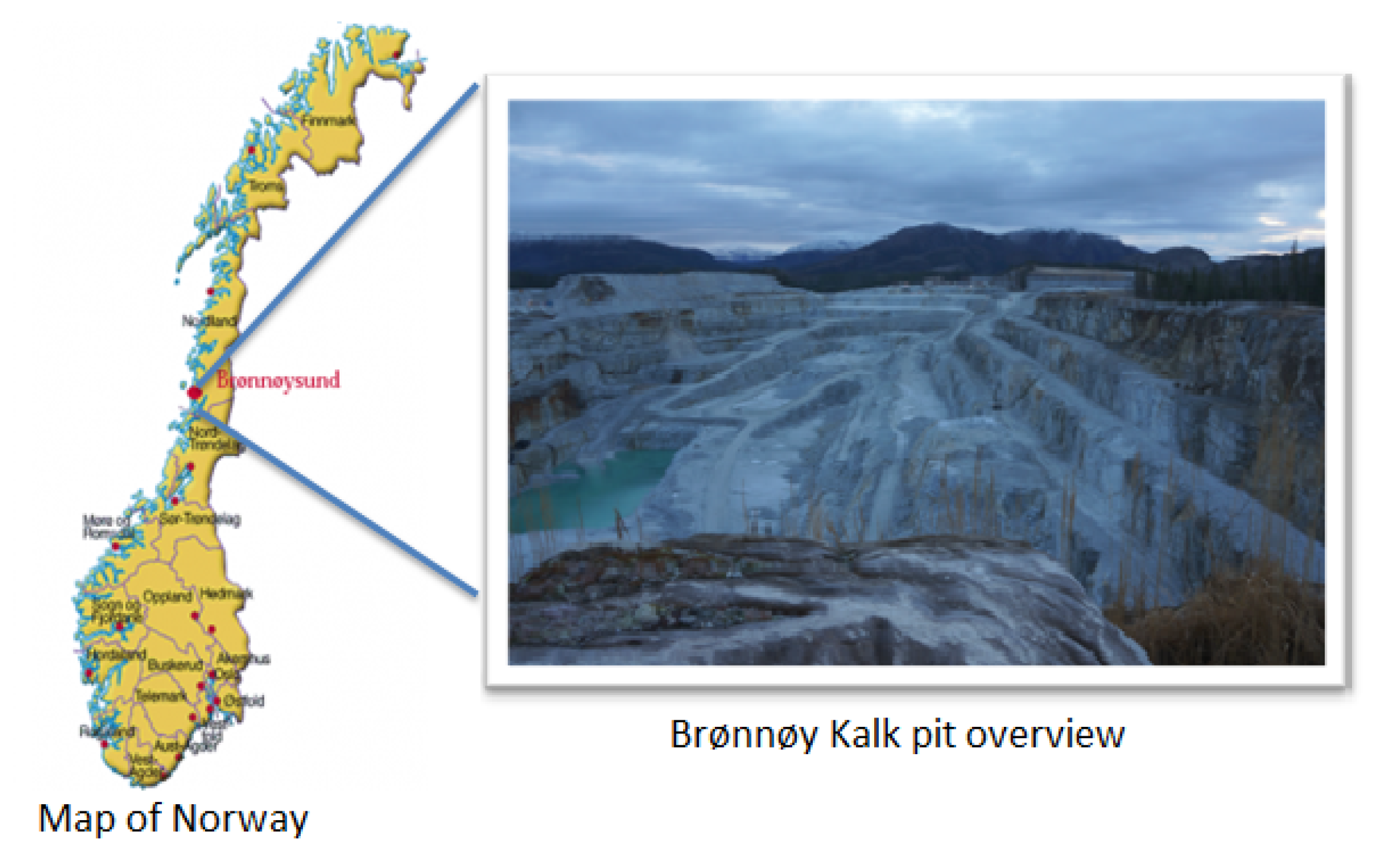
Figure 2.
Penetration rate, rotation pressure and dampening pressure inside marble intrusion along with OTV image.
Figure 2.
Penetration rate, rotation pressure and dampening pressure inside marble intrusion along with OTV image.

Figure 3.
On the left is the map of the mine with location of the selected blasts (orientation with north up). On the right is the position of particular boreholes in each blast that is selected for this study. The selected boreholes are highlighted with orange color.
Figure 3.
On the left is the map of the mine with location of the selected blasts (orientation with north up). On the right is the position of particular boreholes in each blast that is selected for this study. The selected boreholes are highlighted with orange color.

Figure 4.
OTV images of three selected boreholes, the plot adjacent to each image is a numerical representation of the image’s color difference.
Figure 4.
OTV images of three selected boreholes, the plot adjacent to each image is a numerical representation of the image’s color difference.
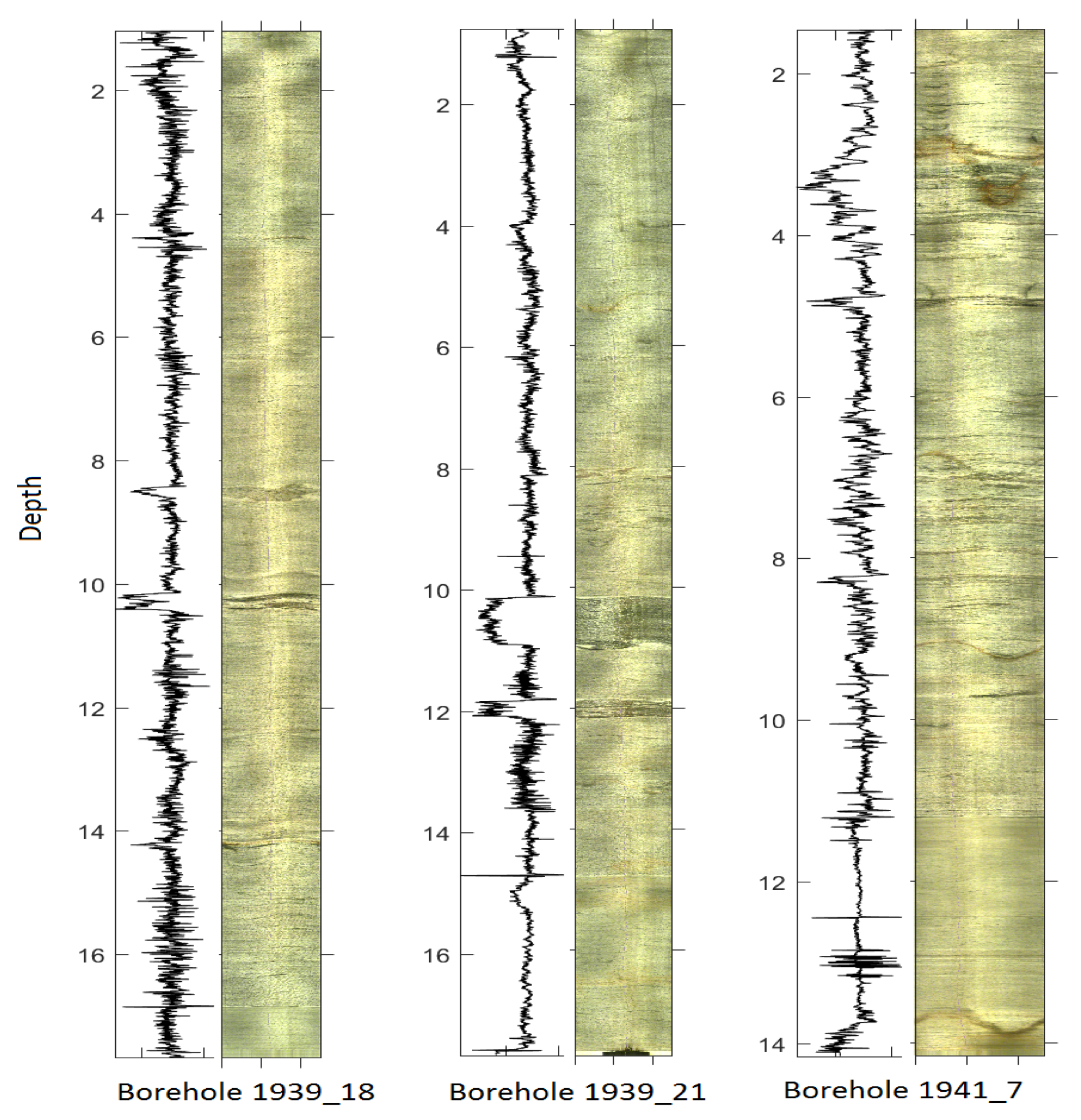
Figure 5.
Illustration of Markov chain realizations when there are three possible rock classes. Left: The Markov chain always goes through class 2 from class 1 to 3, and has a large probability of staying in class 1. Right: The Markov chain transitions can take all combinations and changes in class occur relatively often.
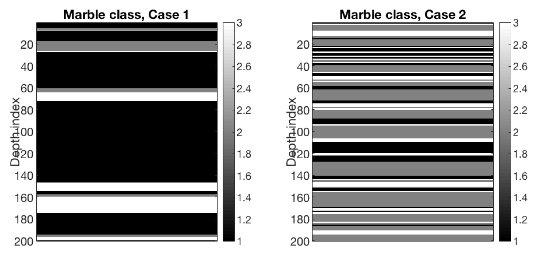
Figure 6.
Illustration of likelihood models for bivariate MWD data and with three rock classes. Left: Difficult to classify the rock class from data. Right: Easy to classify rock class from data.
Figure 6.
Illustration of likelihood models for bivariate MWD data and with three rock classes. Left: Difficult to classify the rock class from data. Right: Easy to classify rock class from data.

Figure 7.
HMM set up for the hidden rock classes and the MWD data.

Figure 8.
MWD data along with OTV images for each borehole: (a) 1939-18; (b) 1939-21; (c) 1941-7.


Figure 9.
MAP predictors using different combinations of MWD data.

Figure 10.
From left to right: Depth plot of TGAM (cps), K (%), U (ppm), Th (ppm), MSUS, and MAPPRD and MAPPR and a zoomed OTV image of borehole 1939-21.
Figure 10.
From left to right: Depth plot of TGAM (cps), K (%), U (ppm), Th (ppm), MSUS, and MAPPRD and MAPPR and a zoomed OTV image of borehole 1939-21.
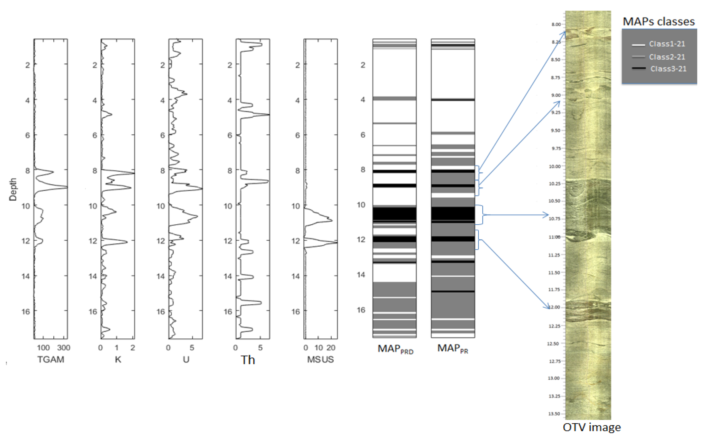
Figure 11.
From left to right: Depth plot of TGAM (cps), K (%), U (ppm), Th (ppm), MSUS, MAP estimator with penetration rate, rotation pressure and dampening pressure and the OTV image for borehole 1939-18.
Figure 11.
From left to right: Depth plot of TGAM (cps), K (%), U (ppm), Th (ppm), MSUS, MAP estimator with penetration rate, rotation pressure and dampening pressure and the OTV image for borehole 1939-18.
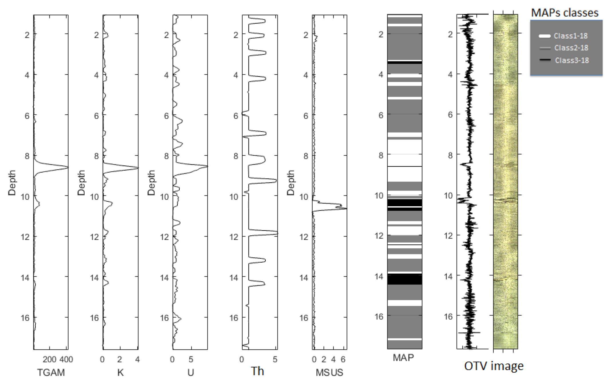
Figure 12.
From left to right: TGAM (cps), K (%), U (ppm), Th (ppm), MSUS, MAP estimator with penetration rate, rotation pressure and dampening pressure and the OTV image for borehole 1941-7.
Figure 12.
From left to right: TGAM (cps), K (%), U (ppm), Th (ppm), MSUS, MAP estimator with penetration rate, rotation pressure and dampening pressure and the OTV image for borehole 1941-7.
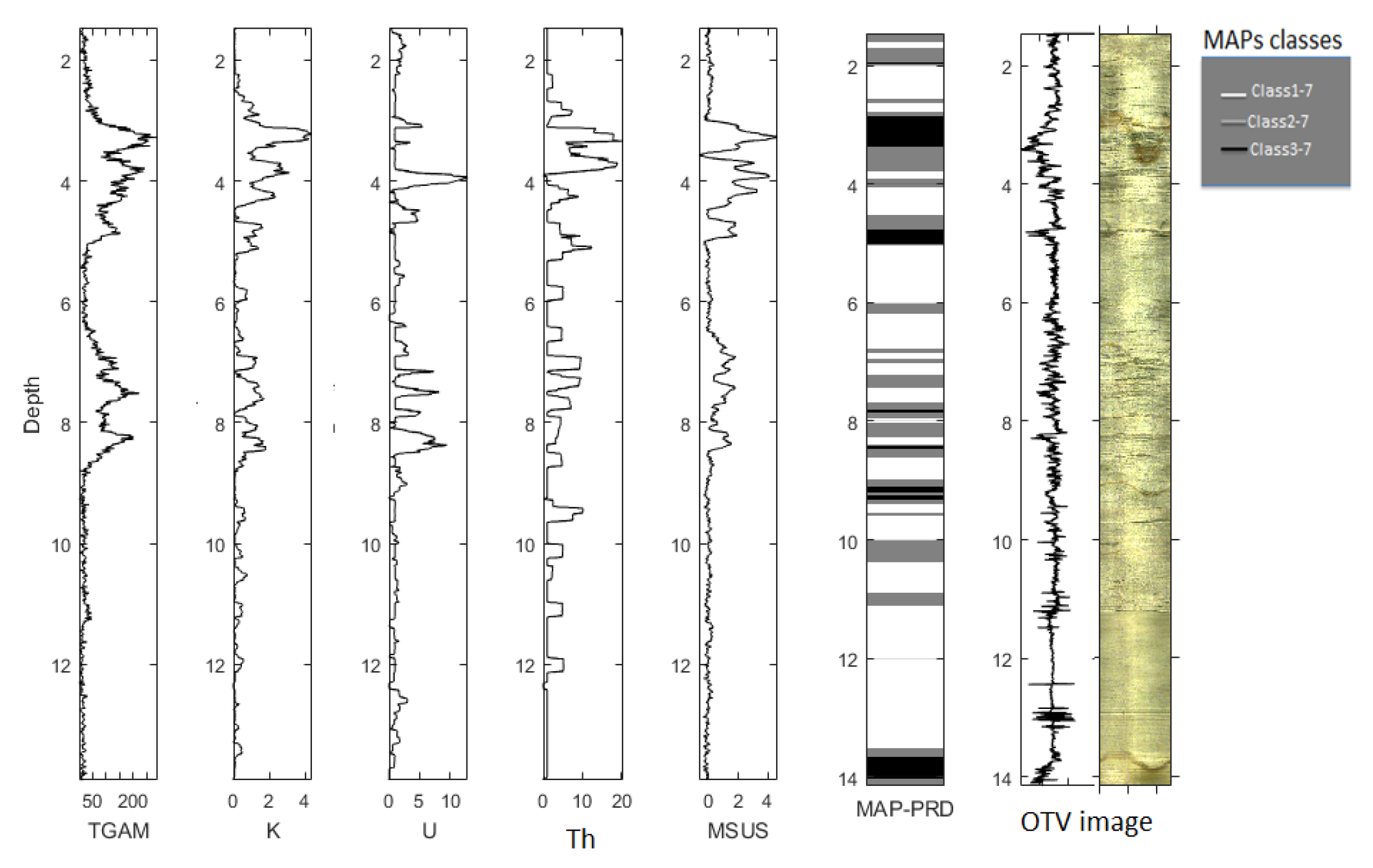
Figure 13.
Likelihood model of the Gaussian distribution represented by 3 ellipses contours using the combination of EM estimated parameters values of penetration rate, rotation pressure and dampening pressure together with corresponding scatter plots for borehole 1939-21.
Figure 13.
Likelihood model of the Gaussian distribution represented by 3 ellipses contours using the combination of EM estimated parameters values of penetration rate, rotation pressure and dampening pressure together with corresponding scatter plots for borehole 1939-21.

Figure 14.
Likelihood model of the Gaussian distribution represented by 3 ellipse contours using the combination of EM estimated parameters values of penetration rate, rotation pressure and dampening pressure together with corresponding scatter plots for borehole 1939-18.
Figure 14.
Likelihood model of the Gaussian distribution represented by 3 ellipse contours using the combination of EM estimated parameters values of penetration rate, rotation pressure and dampening pressure together with corresponding scatter plots for borehole 1939-18.
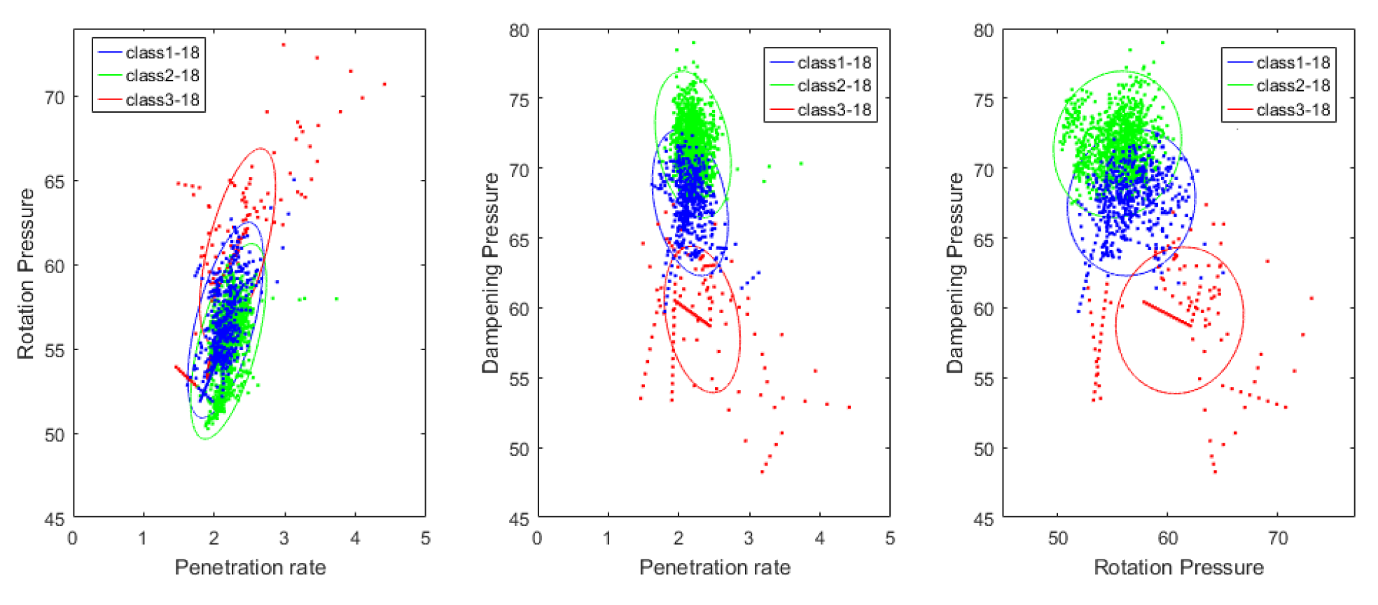
Figure 15.
Likelihood model of the Gaussian distribution represented by 3 ellipses contours using the combination of EM estimated parameters values of penetration rate, rotation pressure and dampening pressure together with corresponding scatter plots for borehole 1941-7.
Figure 15.
Likelihood model of the Gaussian distribution represented by 3 ellipses contours using the combination of EM estimated parameters values of penetration rate, rotation pressure and dampening pressure together with corresponding scatter plots for borehole 1941-7.
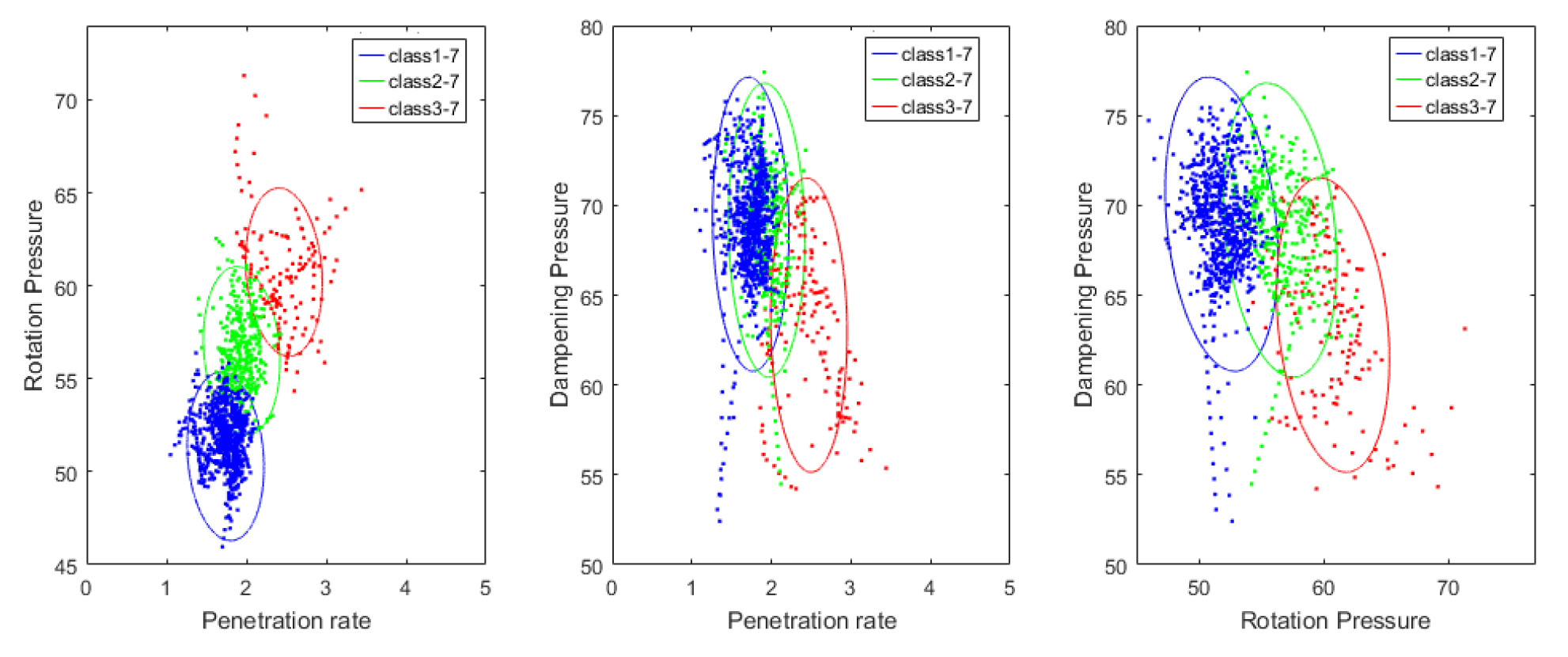
Figure 16.
On left is the densities of TGAM inside each class in the classification and on right is the densities of MSUS inside each class in the classification for the borehole 1939-21.
Figure 16.
On left is the densities of TGAM inside each class in the classification and on right is the densities of MSUS inside each class in the classification for the borehole 1939-21.
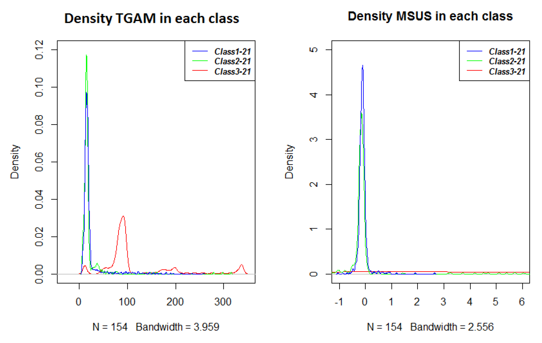
Figure 17.
On left is the densities of TGAM inside each class in the classification and on right is the densities of MSUS inside each class in the classification for the borehole 1939-18.
Figure 17.
On left is the densities of TGAM inside each class in the classification and on right is the densities of MSUS inside each class in the classification for the borehole 1939-18.

Figure 18.
On left is the densities of TGAM inside each class in the classification and on right is the densities of MSUS inside each class in the classification for the borehole 1941-7.
Figure 18.
On left is the densities of TGAM inside each class in the classification and on right is the densities of MSUS inside each class in the classification for the borehole 1941-7.


Table 1.
Mean and standard deviation of MWD data in each boreholes. Standard deviation in parenthesis.
Table 1.
Mean and standard deviation of MWD data in each boreholes. Standard deviation in parenthesis.
| MWD | 1939-18 | 1939-21 | 1941-7 |
|---|---|---|---|
| Penetration rate (m/s) | 2.20(0.22) | 2.11(0.28) | 1.88(0.31) |
| Percussion pressure (Bar) | 189.67(5.97) | 189.35(5.50) | 188.39(6.56) |
| feed pressure (Bar) | 87.69(3.95) | 87.95(3.51) | 87.34(4.55) |
| Flush air pressure (Bar) | 8.36(0.90) | 8.12(0.50) | 6.77(0.52) |
| Rotation pressure (Bar) | 56.28(2.83) | 53.36(3.35) | 54.17(3.65) |
| Dampening pressure (Bar) | 69.68(3.81) | 70.44(3.32) | 68.22(3.83) |
Table 2.
Average penetration rate (Pen rate), rotation pressure (Rot press), dampening pressure (Damp press), magnetic susceptibility (MSUS) and total gamma (TGAM) and assigned class characteristic of each class.
Table 2.
Average penetration rate (Pen rate), rotation pressure (Rot press), dampening pressure (Damp press), magnetic susceptibility (MSUS) and total gamma (TGAM) and assigned class characteristic of each class.
| Class | Pen Rate | Rot Press | Damp Ress | MSUS | TGAM | Assigned Class |
|---|---|---|---|---|---|---|
| Class1-18 | 2.2 | 57.7 | 67.5 | −0.1 | 16.6 | Pure Marble |
| Class2-18 | 2.2 | 55.4 | 71.7 | 0 | 40.7 | Pure Marble |
| Class3-18 | 2.3 | 61.8 | 59.2 | 1.2 | 46.7 | Fracture/small intrusion |
| Class1-21 | 2.1 | 51.4 | 70.4 | −0.1 | 22.2 | Pure Marble |
| Class2-21 | 2.3 | 55.8 | 71.3 | 0.5 | 20.1 | Pure Marble |
| Class3-21 | 1.6 | 58.2 | 67.6 | 8.9 | 116.5 | Hard Intrusion |
| Class1-7 | 1.7 | 51.8 | 69.0 | 0.3 | 43.5 | Pure Marble |
| Class2-7 | 1.9 | 56.5 | 68.6 | 0.5 | 71.5 | Impure Marble |
| Class3-7 | 2.5 | 60.7 | 63.3 | 0.9 | 90.8 | Fracture |
© 2018 by the authors. Licensee MDPI, Basel, Switzerland. This article is an open access article distributed under the terms and conditions of the Creative Commons Attribution (CC BY) license (http://creativecommons.org/licenses/by/4.0/).
Share and Cite
MDPI and ACS Style
Vezhapparambu, V.S.; Eidsvik, J.; Ellefmo, S.L. Rock Classification Using Multivariate Analysis of Measurement While Drilling Data: Towards a Better Sampling Strategy. Minerals 2018, 8, 384. https://doi.org/10.3390/min8090384
AMA Style
Vezhapparambu VS, Eidsvik J, Ellefmo SL. Rock Classification Using Multivariate Analysis of Measurement While Drilling Data: Towards a Better Sampling Strategy. Minerals. 2018; 8(9):384. https://doi.org/10.3390/min8090384
Chicago/Turabian StyleVezhapparambu, Veena S., Jo Eidsvik, and Steinar L. Ellefmo. 2018. "Rock Classification Using Multivariate Analysis of Measurement While Drilling Data: Towards a Better Sampling Strategy" Minerals 8, no. 9: 384. https://doi.org/10.3390/min8090384
Note that from the first issue of 2016, this journal uses article numbers instead of page numbers. See further details here.