Comparison of Wet and Dry Grinding in Electromagnetic Mill
by
 , and
, and
Szymon Ogonowski
1,* ,
,
Marta Wołosiewicz-Głąb
2,
Zbigniew Ogonowski
1,
Dariusz Foszcz
2 and
Marek Pawełczyk
1 1
Institute of Automatic Control, Silesian University of Technology Gliwice, 44-100 Gliwice, Poland
2
Department of Environmental Engineering and Mineral Processing, Faculty of Mining and Engineering, AGH University of Science and Technology, 30-059 Krakow, Poland
*
Author to whom correspondence should be addressed.
Minerals 2018, 8(4), 138; https://doi.org/10.3390/min8040138
Submission received: 19 January 2018
/
Revised: 20 March 2018
/
Accepted: 27 March 2018
/
Published: 29 March 2018
(This article belongs to the Special Issue Sustainable Mineral Processing Technologies)
Abstract
:Comparison of dry and wet grinding process in an electromagnetic mill is presented in this paper. The research was conducted in a batch copper ore grinding. Batch mode allows for precise parametrization and constant repetitive conditions of the experiments. The following key aspects were tested: processing time, feed size, size of the grinding media, mass of the material and graining media, and density of the pulp. The particles size distribution of the product samples was analyzed in the laboratory after each experiment. The paper discusses the experimental results as well as the concept of dry and wet grinding and classification circuits for the electromagnetic mill. The main points of the discussion are the size reduction effectiveness and power consumption of the entire system.
1. Introduction
Comminution is one of the most energy-consuming technological processes, which aims to bring the material to the desired particle size [1,2,3]. The analysis of comminution consists of establishing the relations between the particle size distribution of products, the physical properties of the material, the comminution energy consumption and the parameters of the machines [4]. Comminution of raw material is carried out for two main reasons [1,5]: obtaining a final product, according to the requirements (main operation in the case of aggregates) and, mineral liberation, that is, bringing the material to such a state that it liberates the injection of the useful ingredient from the gangue (preparatory operation to a beneficiation process). Comminution of raw materials is widely used in many industries starting from mineral processing to the chemical, construction, food, cosmetic and pharmaceutical industries.
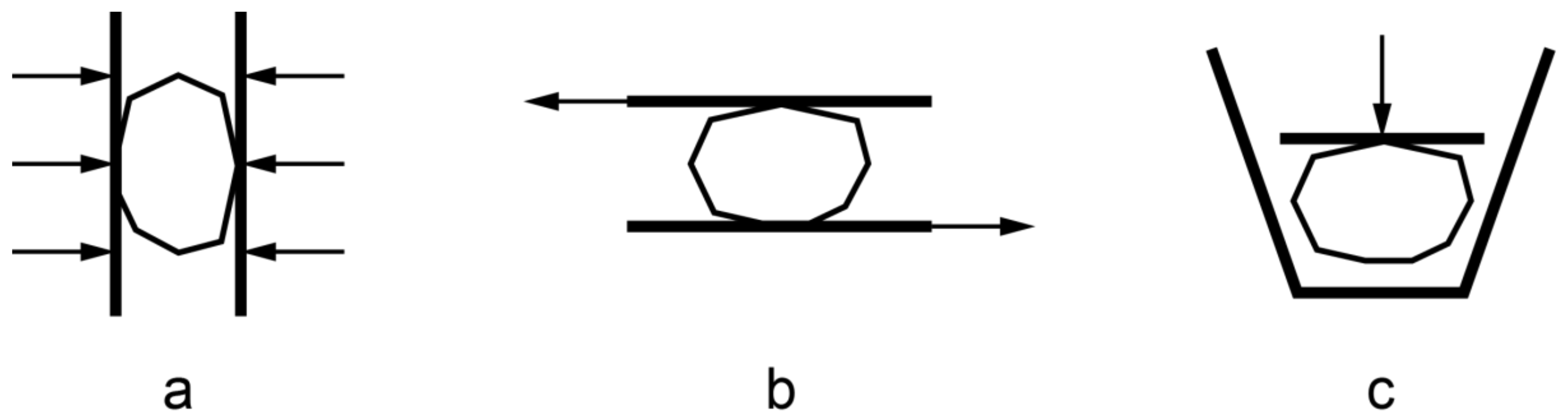
Generally, the comminution can be carried out mechanically and chemically. Mechanical comminution is the result of the operation of external forces or special forces on the material, while chemical comminution leads to the removal of part of the particles by dissolving, digesting or forming a different substance. Mechanical comminution is performed for dividing individual particles of material into smaller parts by smashing, breaking, attrition, pealing, cutting, crushing and other actions. Figure 1 shows three models of particle size reduction in mechanical treatment which follow from the type of machine used for a specific comminution operation. The choice of the machine is usually determined by the feed particles size and the requirements for the product obtained as a result of grinding. These issues are closely related to the efficiency of comminution machines [6,7]. Conventional grinding of mineral raw materials is carried out by crashing of the material using grinding media which refers to the model (b) in Figure 1. There is no shape control of the obtained particles, which often results in low technological value of the product.
This research particularly concerns ultra-fine comminution, which is a high energy consuming process. Conventional devices, such as tumbling ball mill, limit power consumption which follows form physical constraints such as, e.g., speed or grinding media size restrictions. In turn, the quality of the product decreases. For example, at low speed, large grinding media in a tumbling mill generate mainly impact and abrasive stresses, which, for micron- or sub-micron-size particles, do not work well. Thus, mineral processing society and device manufacturers constantly strive to develop less energy-intensive, more efficient solutions, with possibility to precisely define of the product properties such as shape and particle size [8]. This particularly concerns the case of the hard-to-enrich non-ferrous ores where one of the most important directions for modern technologies are new solutions designed for ore grinding to obtain grain sizes in the range of micrometers and development of conditions for effective beneficiation within such grain size [9].
A novel solution, the electromagnetic mill (EMM) can face the above problems. Small ferromagnetic particles which serve as the grinding media in EMM are put into motion in rotating electromagnetic field and devote EMM to ultra-fine comminution. Mainly model (a) and partially model (b) presented in Figure 1 characterize EMM performance what influence the shape of the product particles. The most exciting property of EMM is very short processing time and relatively easy optimization of EMM energy consumption.
EMM allows the use of both of the two principal methods of grinding: dry and wet. This paper presents a research concerning comparison of these two technologies used in EMM installation. The essential advantages of wet grinding over dry one are as follows [10]:
- lower energy consumption per unit of mass,
- better efficiency of the mill,
- no dust,
- lower noise.
Disadvantages compared to dry grinding:
- the wear on the media and liners is usually considerably greater,
- less material in the range of the very small particle size is produced,
- drying the comminuted material usually needs more expensive dust collecting equipment than raw material drying,
- shut down and switching on procedures are more complex in the wet case therefore the wet process is less convenient for day or single shift operations.
Unique characteristics of raw material emphasize the property of wet or dry technologies. For example, if sulphide minerals are processed, wet grinding is preferred because of the following reasons:
- downstream (wet) processing requirements,
- higher energy efficiencies associated with wet grinding,
- requirement for a low moisture content feed (nominally less than 2% moisture) for dry milling is difficult to fulfill,
- fine sulphides tend to oxidize in the air,
- dry grinding often produces strong agglomerates and incrustation build-ups (depending on the fineness of the grind) which are difficult to subsequently disperse,
- the surface properties of dry ground minerals are different than the same minerals wet ground.
The above short clarification points out the importance of a comparative study of both technologies. At some point it is possible to perform such study in simulations using dedicated models [11,12]. Another approach is to use laboratory, semi-industrial or even industrial set-ups to perform comminution tests. This paper presents results of copper ore grinding tests and investigates the differences between dry and wet grinding technique using EMM. The tests were carried out using the same EMM device, the same time duration and the same grinding media sets. In the wet case, grinding tests were performed for different density of the pulp.
Specific requirements for grinding and classification systems regarding the reduction of energy consumption, the optimal particle size and shape as well as the surface properties cause a need to design a modern system with recirculation of particles which do not meet quality requirements. To make this solution competitive, the system should be appropriate for all kinds of raw materials, configurable and equipped with a suitable measuring and control systems. EMM equipped with properly designed supporting units constitutes installation which meets these expectations This paper covers two objectives: it presents EMM and additional units that create entire installation and it presents experimental results of wet and dry grinding of the exemplary raw material using EMM completed with analysis of chosen factors and indicators of grinding efficiency.
The paper is organized as follows. In Section 2, EMM is described including wet and dry installations. Section 3 presents wet and dry experiments. Laboratory set up and experiments are described. Analyses of the experimental results are presented in Section 4. Chosen factors and indicators are defined and discussed. Energy consumption problems in the EMM installations conclude this section. The paper ends with conclusions and further works.
2. Electromagnetic Mill
2.1. Device Description
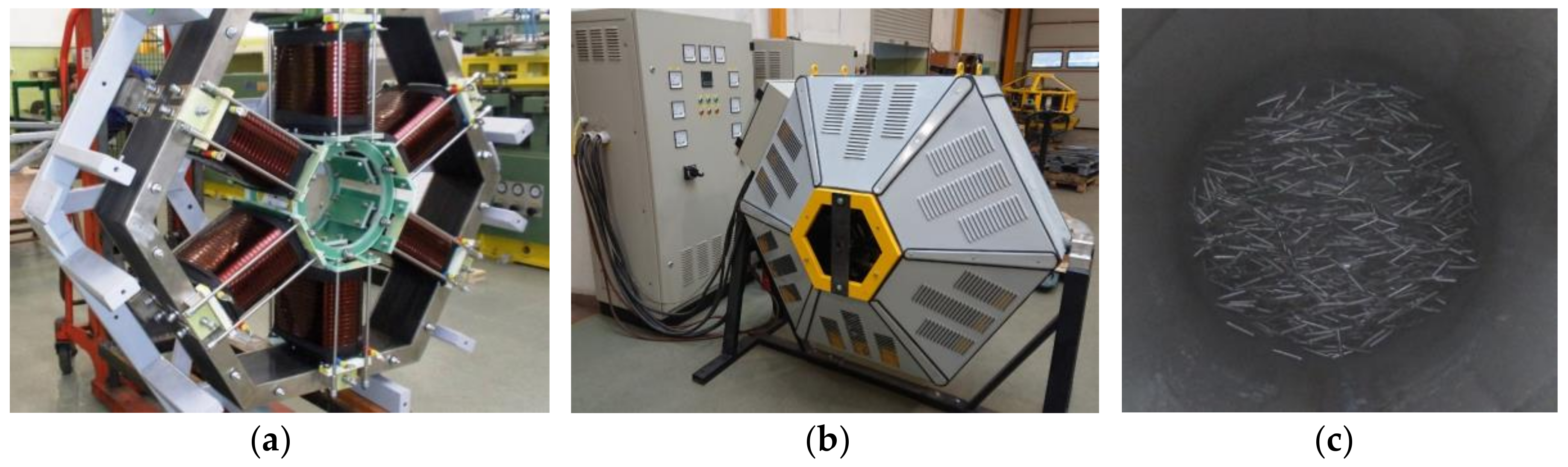
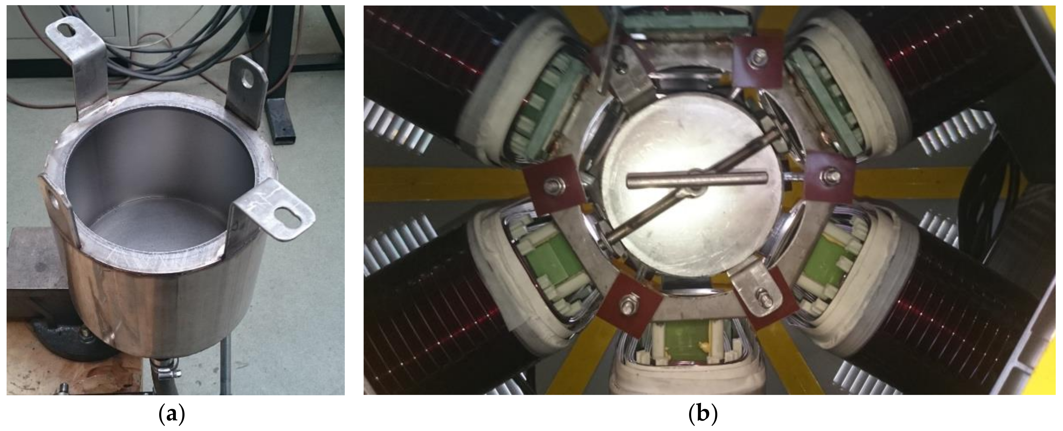
The electromagnetic mill is a novel grinding device, where a rotating electromagnetic field is directly used to move ferromagnetic grinding media in the working chamber [13]. Figure 2 presents an exemplary D200 EMM with a working chamber diameter equal to 200 mm. The working chamber is a non-ferromagnetic tube surrounded by six electromagnets to create electromagnetic (EM) field (Figure 2a). The grinding medium in the form of small ferromagnetic rods fills about 10% of the working chamber volume. The shape and size of the grinding media and the mill parameters were determined by simulations using finite element analysis, to obtain the optimum effectiveness of the magnetic force. The size parameters of the rods depend on the mill diameter and the average feed. It is usually of 1–3 mm of diameter and 10–15 mm of length. When the rotating electromagnetic field is inducted in the working chamber, the medium starts to move. Collisions between the rods and the processed particles cause chaotic movement inside the chamber and increase the grinding effect (Figure 2c). The rotating EM field inducted inside the working chamber keeps the grinding media inside the chamber. However, that it is true only for specific operating frequencies and material flowrate range, thus adequate control of these quantities is required. Physical parameters of the mill, including the working chamber volume, distance between the chamber and inductor, number of inductor cores, etc., have been optimized to maximize the force exerted by the EM field and to minimize the electric energy consumption.
The nature of the grinding process in EMM allows for the control of shape parameters of the product grains. In the first stage of the grinding, the size reduction is performed mostly by breaking and splitting, caused by collisions with the grinding media. When the grain reaches certain size, it begins to abrade by slide on the surface of the grinding media. Such phenomena allow us to obtain sharp grain edges and irregular shapes or more cubic ones with soft edges. Parameters of the grinding process in EMM also influence the reactivity level and other physical properties of the product grains. Thus, EMM becomes significantly competitive to other milling solutions. It requires, however, dedicated grinding and classification circuit and complex control system. Such a system for dry grinding process was developed [14] and patented [15] by the consortium of Polish universities and companies: Silesian University of Technology, AGH University of Science and Technology, ELTRAF Company (EMM producer, Lubliniec, Poland) and AMEplus Company (integrator of automation systems, Gliwice, Poland). Modelling of the air transport paths was carefully studied [16,17,18], classification capabilities were examined [19,20], and control problems were discussed [21,22,23]. Section 2.2 describes the idea of the entire system and describes differences between wet and dry grinding circuits.
2.2. Grinding and Classification Circuit
Literature reports several examples of the electromagnetic mill applications [24], where the working chamber is in a fixed leaning position. Similar solutions were tested at the early stage of the research. The idea assumes leaning position of the working chamber with the mills’ inlet situated higher then outlet. The feed is supplied at the inlet and the leaning position causes sliding of the processed material through the chamber by the gravity force. The main disadvantage of such a solution is foremost the strongly constrained controllability of the sliding speed and, in turn, uncontrolled grinding time. A fixed position also limits throughput control. There are applications with an adjusted angle of the chamber, but still the gravity and the friction determines the functionality of such feeding system.
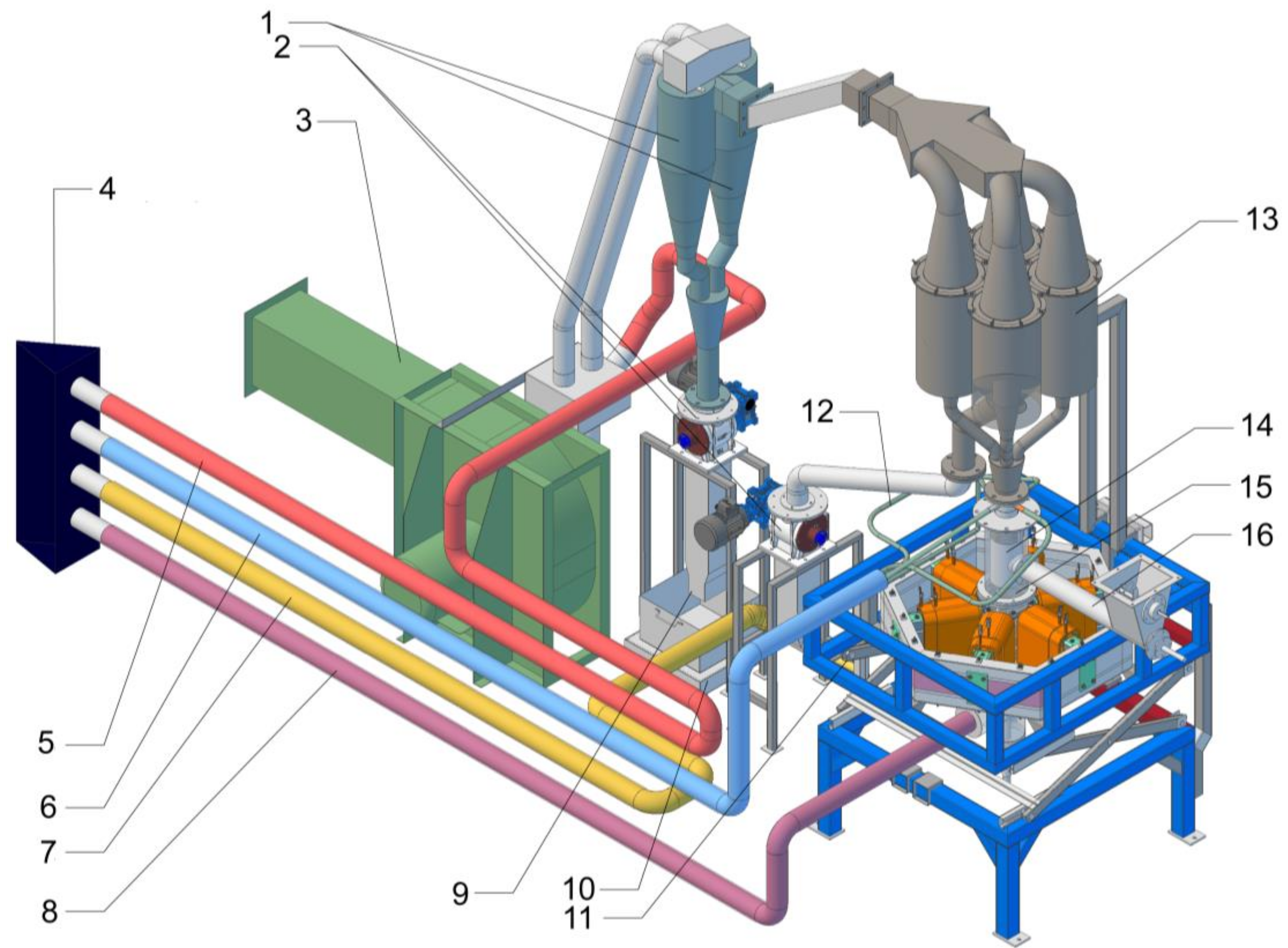
To control the grinding process more precisely and to increase its effectiveness, a dedicated material transport and classification system need to be designed. Preliminary studies with the gravitational material transport outlined the requirements for the dry grinding and classification circuit with pneumatic transport. The idea of such circuit is presented in Figure 3a. It assumes vertical positioning of the working chamber and feed supply from the top of the chamber. Figure 3b presents one of the circuits build in ELTRAF Company for the D200 EMM. Figure 4 presents the 3D model of the installation for better illustration of the particular stream flows in the system. The following description uses labels shown in Figure 4.
Material is fed to the installation by the screw feeder (no. 16) into the preliminary classifier (no. 14) situated above the mill from where larger grains drop down into the working chamber (no. 15) surrounded by 6 electromagnets which generate rotating magnetic field. Material is transported by the pneumatic transporting system. The air stream is taken form intake (no. 4) and exhausted trough the outlet (no. 3) directly connected to the main fan. The main air stream (no. 8) supplies the working chamber from the bottom and swept grinded grains up though to the preliminary classifier (where heavier part is again shifted back into the working chamber) to the main classifier (no. 13) which is parameterized by additional air stream (no. 6). The main classifier is composed of four elements working in parallel. Coarse grains leave the main classifier through the pipe (no. 12) and rotary valve (no. 2) which separates pressure to meet recycle air stream (no. 7) and to be taken back to the working chamber form its bottom side. Fine grains leave the main classifier through its top collector and are pneumatically transported to the cyclone (no. 1) which is composed with two elements working parallel. The product is collected in the bottom part of the cyclone and transported down to the tank by the rotary valve (no. 2) to separate pressure. The recovered air stream is drawn from the cyclone top by the main fan to the collector to which bypass air stream (no. 5) is also attached to reduce the total air flowrate through the working chamber and classifier.
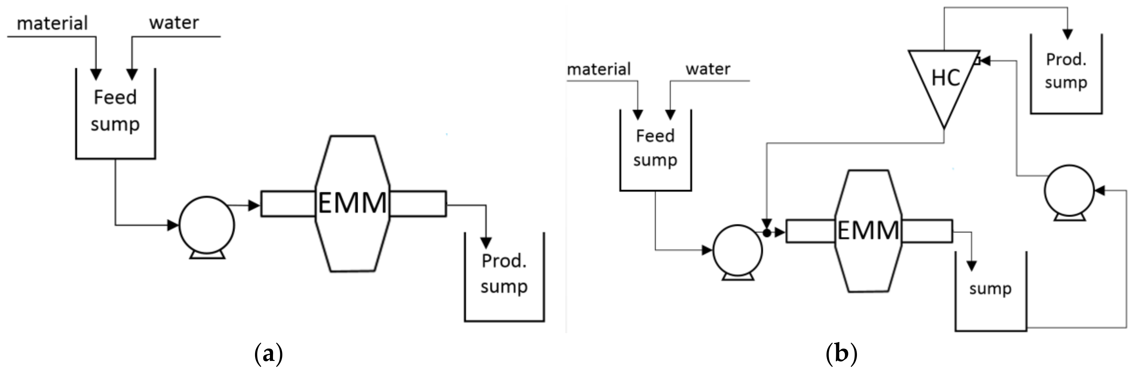
Recently, the authors focused on the dry grinding with pneumatic transport. To compare its effectiveness with wet grinding, a standard open and close circuit was chosen for the preliminary research [25]. Figure 5 represents two concepts of such circuits with and without recycle of coarse material using hydrocyclone (HC).
In the open circuit (Figure 5a) the material suspension is transported by a pump from the feed sump to the working chamber of EMM and then flows to the product sump. In such a solution the grains pass through the working chamber only once and the flowrate needs to be respectively low to ensure proper grinding time. It reduces the mills throughput significantly and sometimes the lowest possible flowrate is not enough for certain grains to reach the desired size. The second solution (Figure 5b) assumes classification of grinding particles in HC. The mills output is pumped from the output sump to the HC input. Fine particles create HC overflow and are directed to the product sump while coarse ones are directed as an underflow, back to the EMM input. Similarly to the additional airstream in the case of dry grinding (no. 6 in Figure 4), it is usually necessary to use an additional pump to increase the flowrate and control the pressure at the HC input [25].
Due to different transport methods, it is difficult to compare the dry and wet grinding process in EMM accurately. That is why the authors decided to perform batch grinding experiments in the first stage of the research. For that purpose, a dedicated laboratory set-up was constructed, where EMM D200 is equipped with a non-ferromagnetic capsule, serving as a working chamber. Section 3 of the article describes the set-up and the experimentation methodology.
3. Wet and Dry Grinding Experiments
3.1. Laboratory Set-Up Description
The efficiency of the grinding process depends on many mineralogical, technological and control variables. In grinding and classification circuits, the operating parameters of the machine (like material and grinding media load, rotating speed, wear off of the mills shell, etc.) are also disturbed by other appliances’ performance. The efficiency of the air blowers or suspension pumps, accuracy of flow or density meters and quality of the control system can significantly influence the final product quality. To eliminate such problems, a laboratory set-up for batch grinding was designed by ELTRAF Company. Figure 6 presents an example of the batch working chamber for EMM D200 in the form of a non-ferromagnetic capsule. The capsule has a cylindrical shape with one removable base that allows us to insert the material and grinding media batch. After the base cover is firmly closed, the capsule is inserted into the mill inside the EM field inductor (Figure 6b). The second base of the capsule has a small valve for safety, due to overpressure (Figure 7a). The mill is equipped with a supply and supervisory cabinet which allows for the process parameters monitoring and control. Energy consumption was measured among the others, using power grid analyser. Based on the on-line measurements, the total energy consumption during each experiment was calculated. The laboratory is also equipped with scale and moisture analyser that allows for the precise preparation of dry and wet batches. For the purpose of experiments, the material batches of limited size range were prepared.
3.2. Experiments Description
The proposed methodology of batch grinding allows for the precise control of the feed parameters in terms of grain size, weight and volume, initial material moisture or density of the pulp. Precise batch of grinding media can also be prepared with certainty that they will not leave the working chamber during experiments. The supervisory control and data acquisition (SCADA) system controls the entire experimental parameters (inverter output frequency, induction level, processing time and temperature among others). Easy access to the batch after the experiment is terminated allows for manual material sampling. It is also possible to emulate the recycle, by separating fine particles after experiments, using dedicated sieves.
The main disadvantage of such methodology is lack of the material flow through the working chamber. In such a case, input velocity of the particles influences the process and results are different than in the batch processing. On the other hand, constant initial conditions are significant if comparison of different mills operating parameters is concerned.
Copper ore obtained from the deposit operated by KGHM (Lubin, Poland) at Legnica-Glogow Copper District (LGOM) was used in the experiments. Material lithological composition included sandstone—49.5%, slate—16.0%, and dolomite—34.4%. In the dry grinding experiments, 24 copper ore samples with a weight of 500 g were processed successively in the working chamber. The volume of the material constitutes 4% of the working chamber volume (WCV). The grinding was carried out for six processing times: 5, 10, 15, 20, 25 and 30 s. Four types of grinding media were used (length (mm)/diameter (mm)): 12/2, 12/1.5, 10/1 and, additionally a mixture of different sizes. During each experiment, the mass of grinding media was equal to 1500 g (9% of WCV). The composition of mixture was as follows: 750 g of 1.5/12 + 450 g of 1/10 + 300 g of 2/12. The electromagnetic mill was operated at the same output frequency 50 Hz. Table 1 gathers the parameters of all 24 dry grinding experiments and Figure 7 presents the working chamber capsule after the grinding experiments.
For the wet grinding experiments, samples of copper ore pulp with the same solids mass (470 g, 3.5% of WCV) were processed. Three different values of pulp density were tested: 1600 kg/m3, 1700 kg/m3 and 1800 kg/m3. To maintain constant solids mass, different values of density were achieved by different volumes of water and in turn different values of pulp samples. The grinding was carried out for 5, 10 and 15 s. Small grinding media with a total weight of 1500 g (9% of WCV) were used for the study. Those parameters followed from the results of dry grinding that are discussed in the next sections. Table 2 gathers parameters for all 9 wet grinding experiments.
3.3. Factors and Indicators for Results Analysis
Samples of grinding product from every experiment were tested in the laboratory for particles size distribution using laser diffraction technique. This technique is currently the world standard in measuring of the particle size, suspensions and emulsions. The particle size analyzer provides reliable and precise results in a timely manner. The particle size distribution measurement is a non-invasive method in a wide micrometric range (0.1–300 μm). In the experiments, the particles dispersion was analyzed for wet and dry modes. It was important to choose the right dispersant, which ensures maximum particle dispersal: water for wet samples and, compressed air in the dry case. The tests were performed using the ANALYSETTE 22 NanoTec (Fritsch, Idar-Oberstein, Germany) analyzer with following instrumental settings: range 10 nm–2000 µm, analysis time 5–10 s, light source: 2× laser diode, 532 nm, infrared (IR) diode, 940 nm, number of detector’s light sensing elements: 75 and dispersion method: air/liquid. The weight of the representative samples was 150 g, and in the case of wet grinding, samples were taken representatively. In the ore processing research, a precise particle size analysis is of particular importance. The particle size distribution of the processed ore is one of the most important parameters determining the correct course of the processing. Proper preparation of the ore in terms of particle size distribution in milling processes guarantees optimum mineral liberation with the lowest possible consumption of electrical energy and utilities, which improves the efficiency of the flotation [26].
On top of graphical comparison of cumulative volume distribution obtained from laser analysis, several indicators were calculated. Two of them are widely known in the literature size reduction factors for d50 and d80 (the intercepts for 50% and 80% of the cumulative volume). The factors were calculated as follows:
where subscript F stands for feed and subscript P stands for product.
The authors proposed another factor based on the surface areas below the cumulative volume curves of the process feed (FAREA) and product (PAREA). In each case, the surface area was calculated using composite trapezoid quadrature for numerical integration [27]. Figure 8 presents an exemplary comparison of surfaces resulting from the given quadrature. One can notice a small integration error in the range from 20 to 80 µm. The error can be noticed due to low number of integration nodes used in the graphical example for better visibility. For the results presented in the following sections there were 36 integration nodes used instead of 9 nodes presented in Figure 8. Compared with the monotonic nature of the cumulative volume curves the integration error is negligible.
The factor SDIFF is calculated as a difference between product area and feed area:
To better express this difference the SNDIFF factor is calculated as a normalized difference between product area and feed area, and is expressed in %:
This indicates the percentage difference between the areas of feed and product. The presented example is calculated for the whole range of grains size. However, it can be easily modified to be calculated for the limited grains size range, e.g., from 100 µm to 200 µm or from dP80 to dF80.
4. Experimental Results Analysis
4.1. Product Parameters
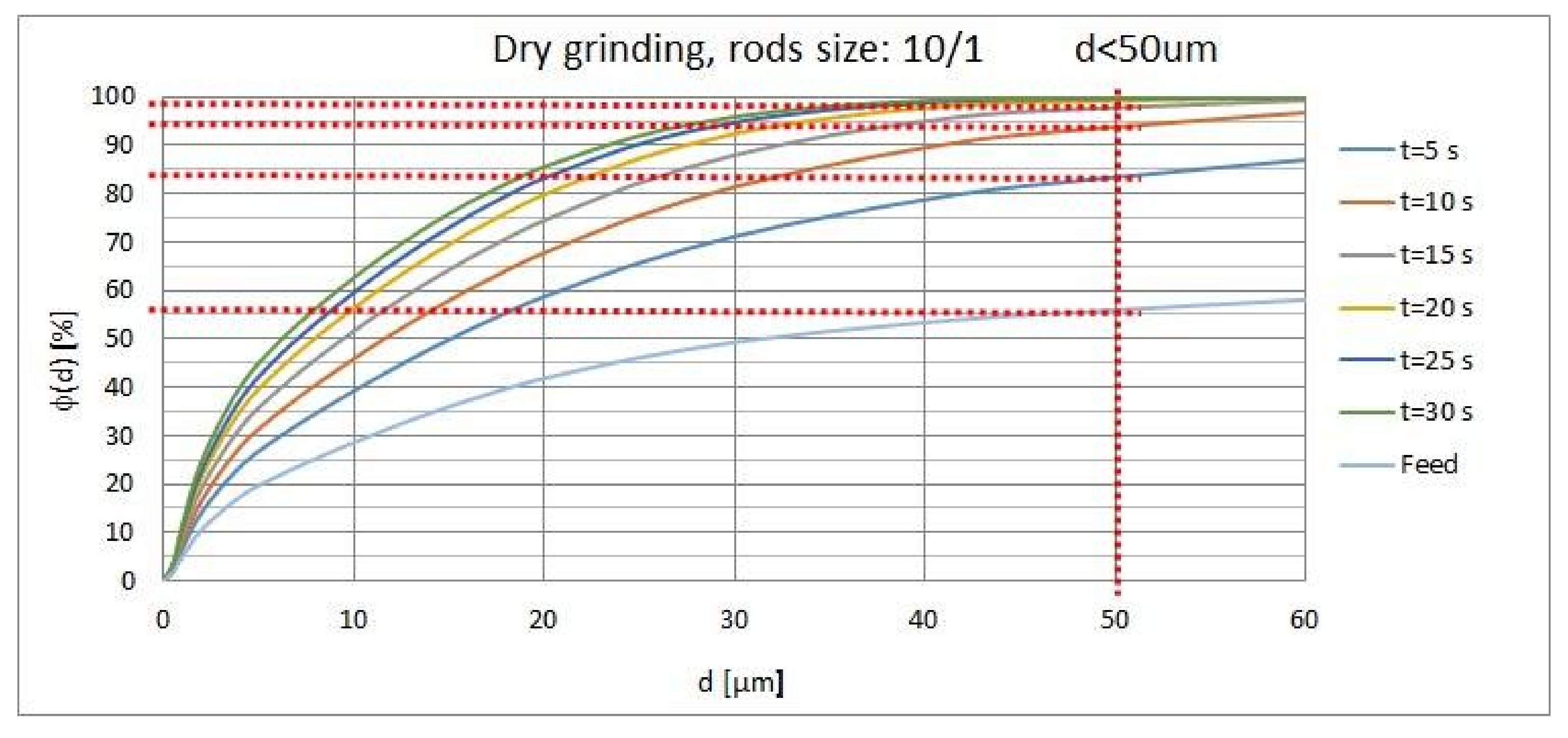
Figure 9 presents the comparison of cumulative volume curve for dry grinding with 10/1 mm rods. For better visibility, the size range was reduced to 0–60 µm. One can notice that the increase in size reduction is most visible when the processing time is increased from 5 to 10 s. A further increase of the processing time does not improve the results significantly.
Figure 9 contains markers for the cumulative volume distribution of grains with size lower than 50 µm. The feed sample has approximately 56% of such grains, 5 s product 84%, 10 s product 94% and all the samples of product for longer time have approximately 98%. Such comparison shows again that the optimal processing time in terms of size reduction and energetic efficiency would be 10 s. The value is accurate for the given material parameters and the EMM model (D200).
Figure 10 presents the results of the same experiment, focusing on the value of the d80 parameter. It shows even more clearly how the size reduction increase drops for longer processing time. The size range in that case was reduced further for better visibility.
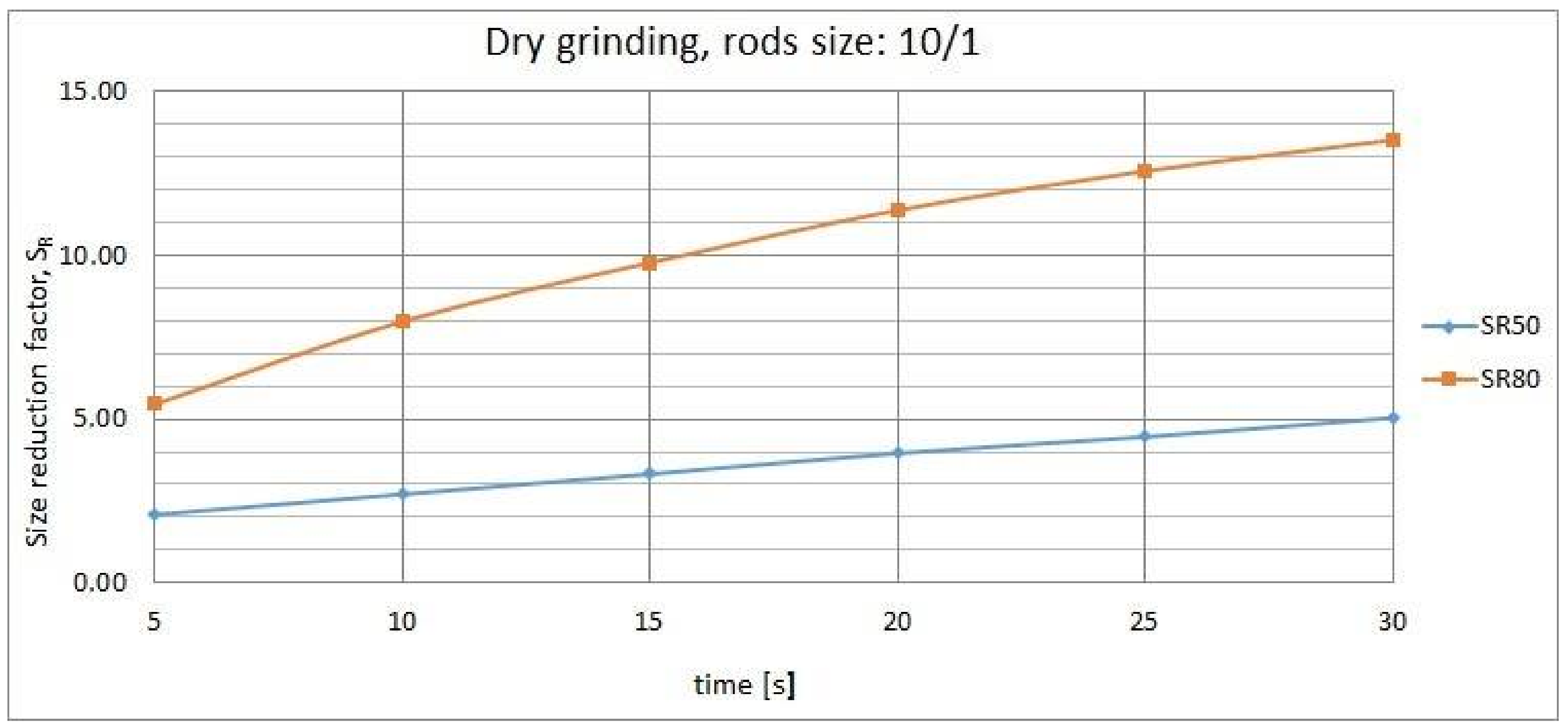
Such an effect is obviously seen when cumulative volume curves are graphically compared. However, it is not so clearly visible when using standard size reduction factors SR50 and SR80 (Figure 11). The slope becomes higher between 5–10 s and 10–15 s which is clearer for SR80, but still the curves presented in Figure 11 can be treated as linear. Of course, they are monotonic in time and for wider range of processing time one should notice a saturation of SR factor, but it was not examined in the present research. The precise values of the SR factors were gathered in Table 3.
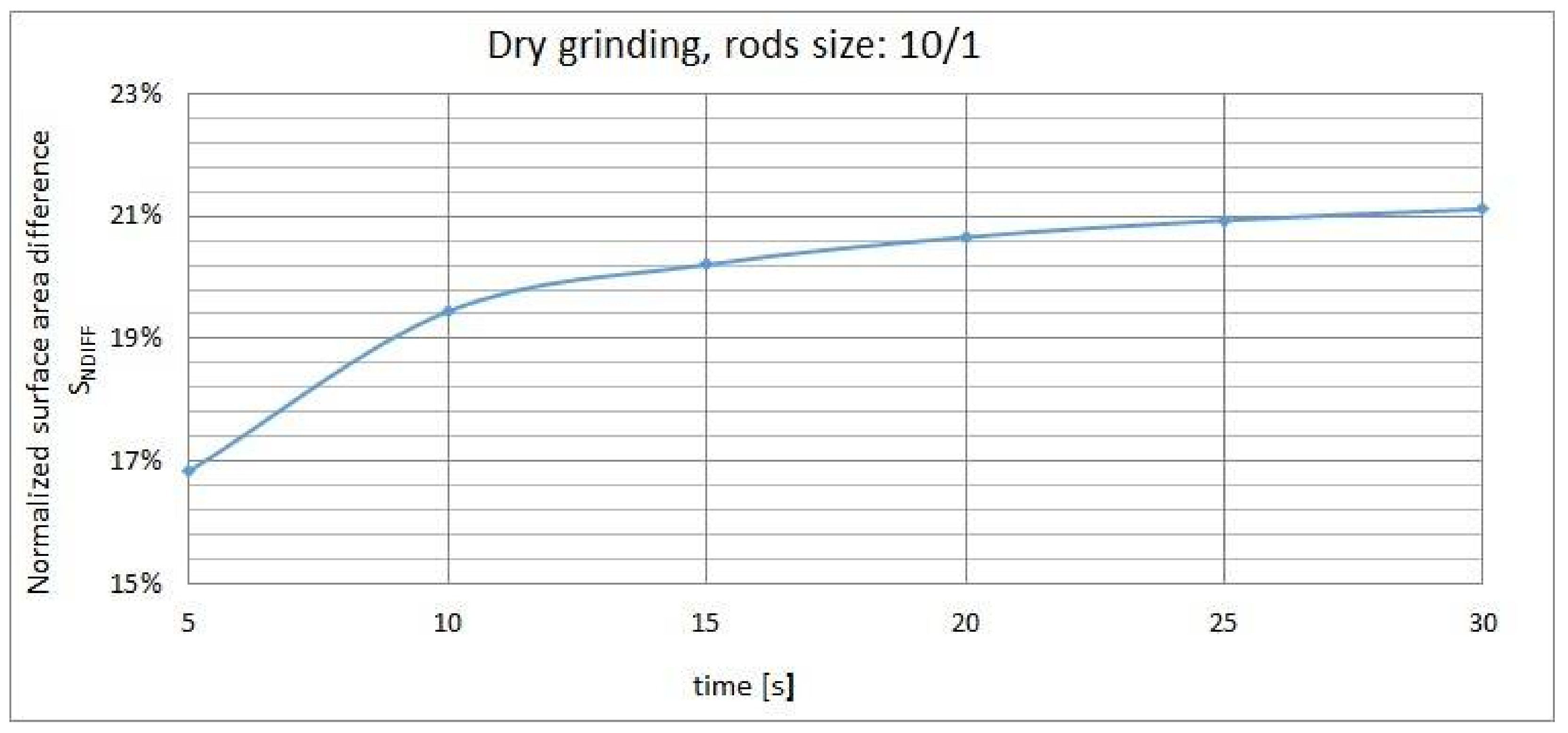
The SNDIFF factor allows us to describe in a numerical way the effect of size reduction efficiency deterioration. Figure 12 presents the SNDIFF changes, taking into account the whole grain size range. It expresses the percentage increase of the surface below the cumulative volume curve. The graining efficiency saturation is clearly visible using this factor.
Table 3 gathers all the important factors used to evaluate the research results for the dry grinding with the 10/1 mm rods example. Maximal relative standard deviation (RSD) was estimated according to the theory of errors [27] for division, trapezoid integration and subtraction with assumed laser diffraction technique accuracy according to ISO13320 [28]. One can notice the monotonic nature of the factors changes with processing time and the saturation of these changes. Such a result allows for throughput planning for the grinding and classification circuit and estimation of the energy efficiency of the process. Measured energy consumption per experiment and estimated specific energy are reported in Table 3 to give some measure of comparison with classic milling solutions. Specific energy was estimated based on the total energy consumption and processed material mass. Energetic efficiency comparison is one of the important issues that will be studied further by authors. Equally important are specific shape and other physical properties of the product grains.
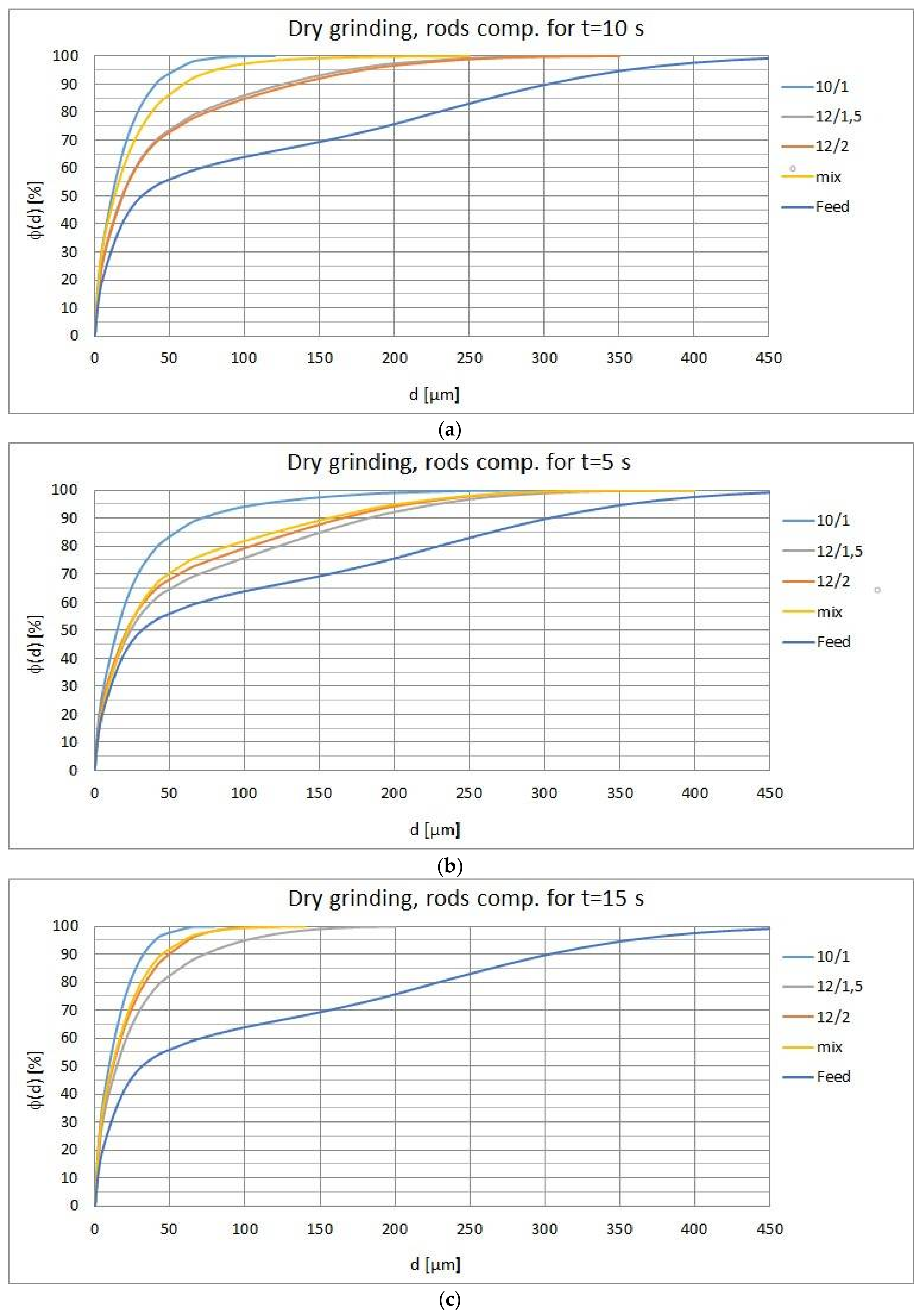
The results obtained from other grinding media (rods) sizes were similar in terms of efficiency monotonic growth and saturation. The authors would like to focus on the results for 10/1 mm rods, because such rods allowed us to obtain the best size reduction factors. Figure 13a compares the result for the optimal 10 s processing time for all types of grinding media sizes. One can notice that the mixture of rods was only similarly efficient when compared with 10/1 mm rods. Again, this is true for the chosen material initial size and the mills’ physical parameters. One of the reasons for this is that the optimal size of the grinding media will be different for different mill sizes (see Section 2.1).
It was observed that, in the case of 5 s processing time (Figure 13b), the efficiency of the mixture was similar to that of the larger rods and when the processing time was increased (Figure 13c) the efficiency of all rods asymptotically approached the level of 10/1 mm rods. This may indicate that the difference noticed for smaller times was caused by slower rods velocity in the first seconds of the experiments (in the case of larger rods). When the rods reached operating velocity, their efficiency was similar. The authors assume that this effect will not occur in the continuous grinding circuit so final conclusions for such applications require further studies.
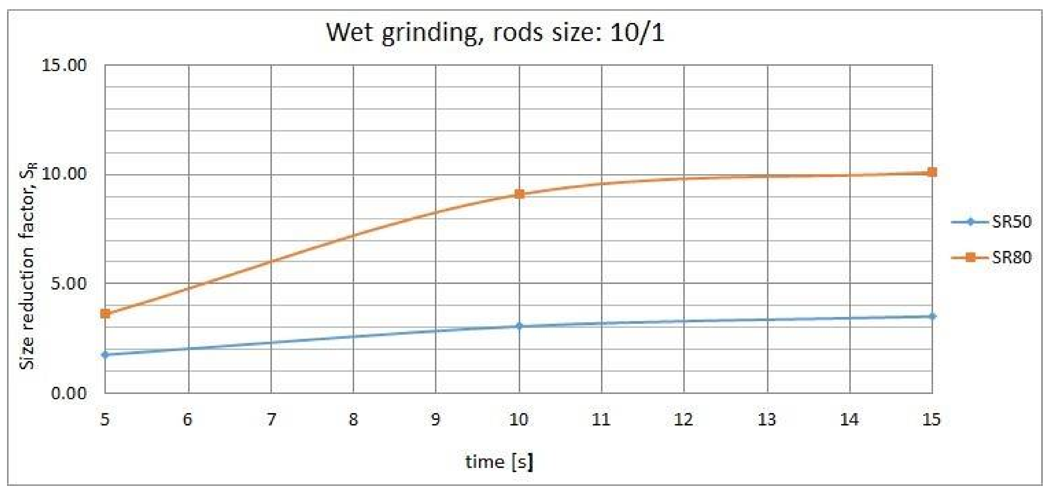
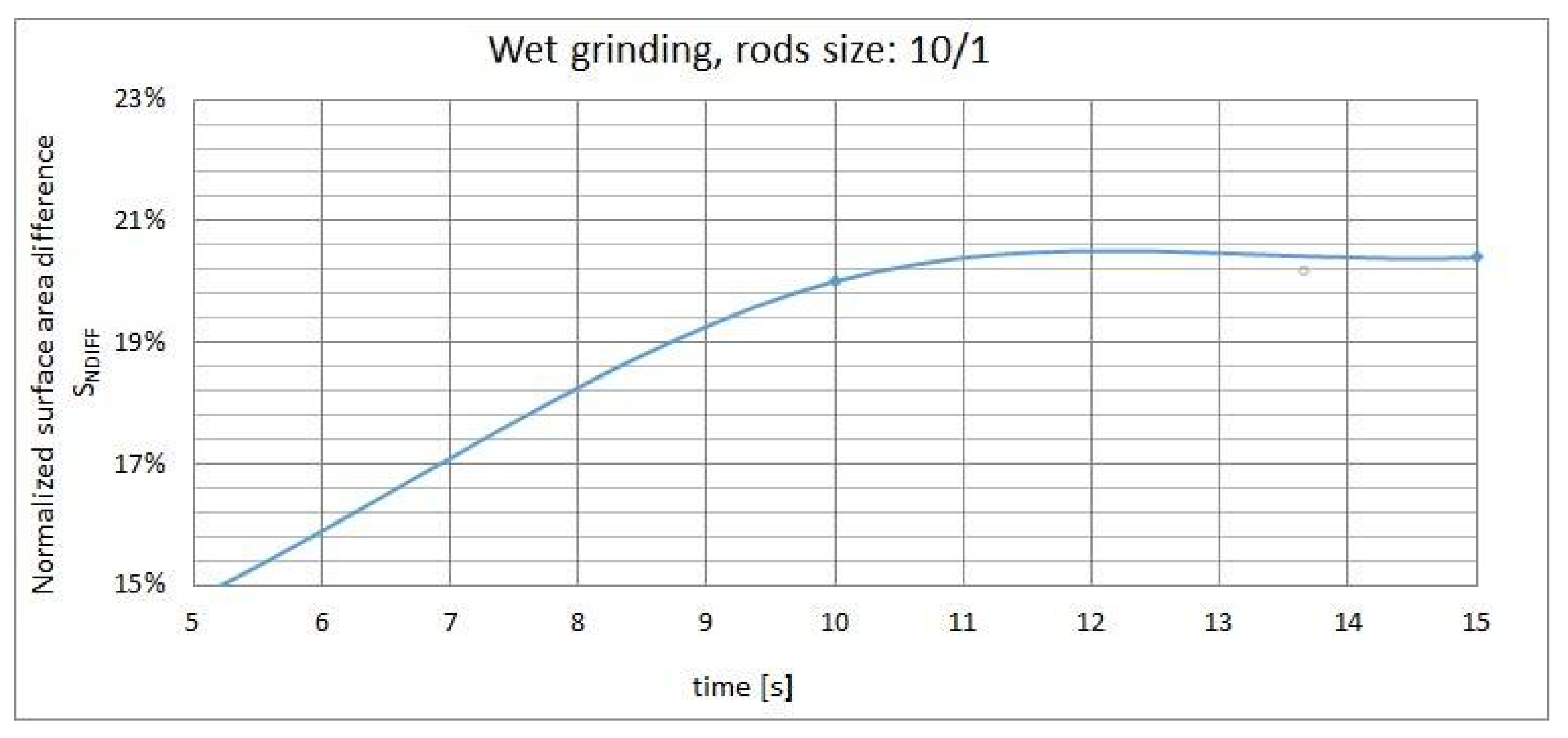
Similar analysis was performed for wet grinding experiments. Figure 14 and Figure 15 present the changes of SR and SNDIFF factors with the increase of processing time. Taking into account the results of the analysis for dry grinding, the research was performed only for three processing times: 5, 10 and 15 s. Again, the results were similar in terms of monotonic nature and optimal processing time for all three of tested densities. Table 4 gathers the size reduction factors for the wet experiments. One can notice the same relation between the different factors when compared to the dry grinding.
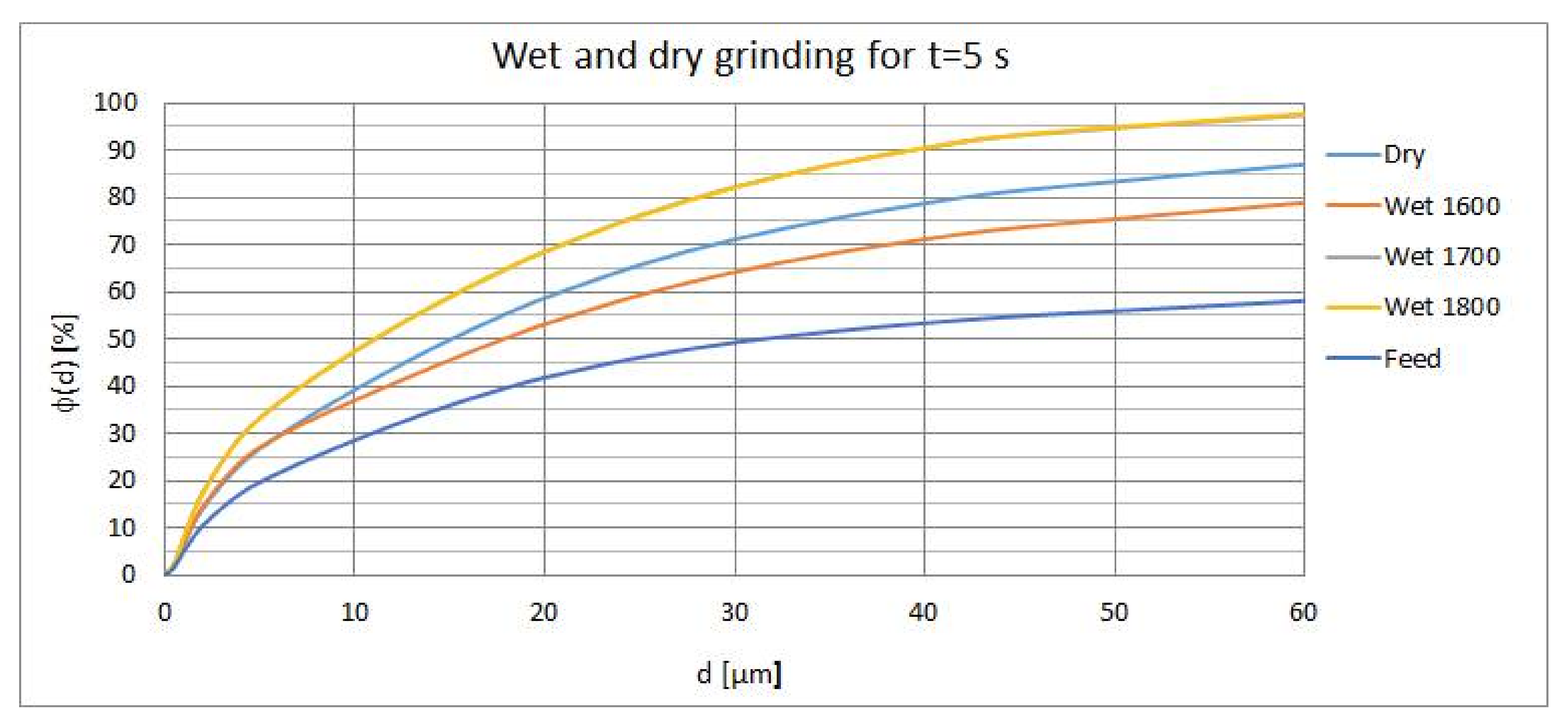
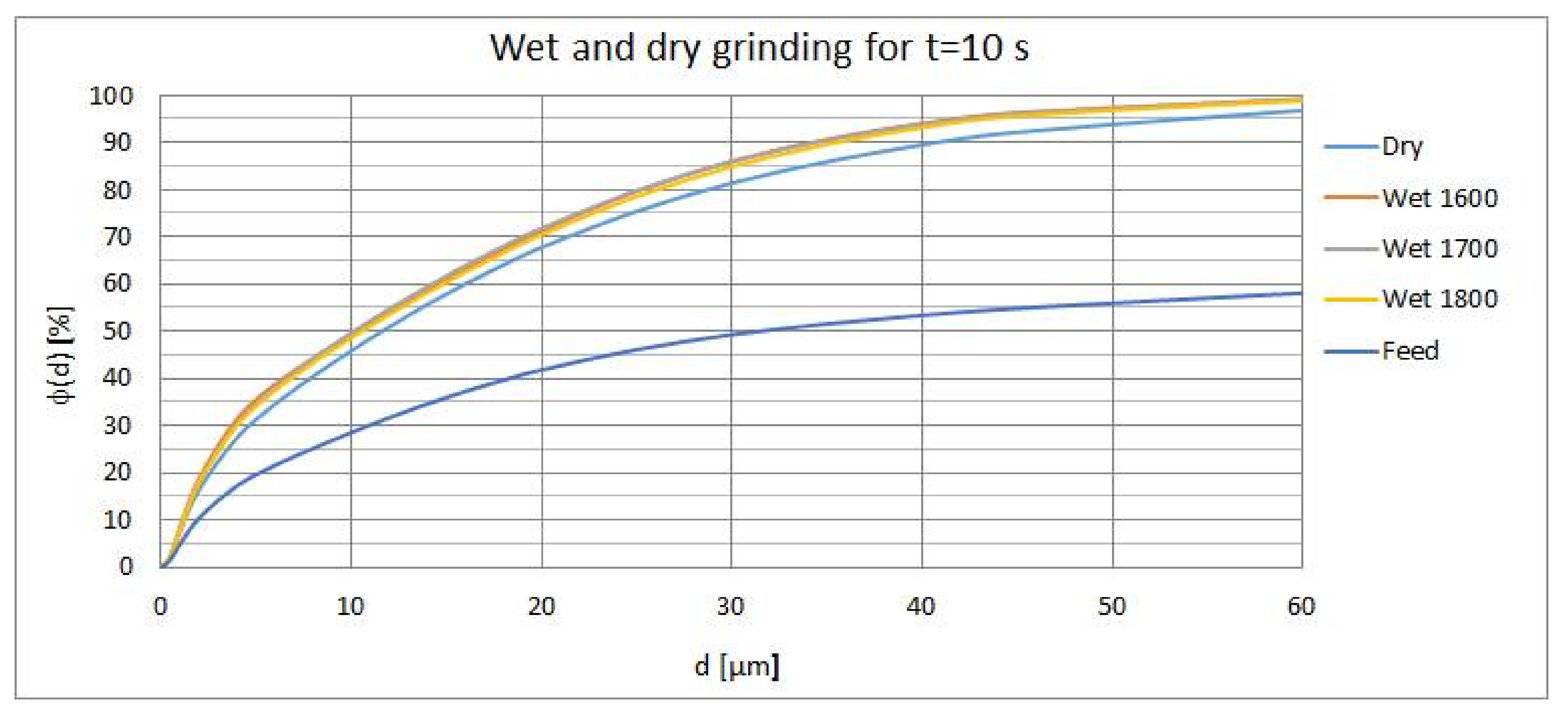
Figure 16 and Figure 17 present the comparison of the cumulative volume curves for dry and wet grinding process. For better visibility, only the range 0–60 µm of the particle size was compared. One can notice slightly better values of all grinding effectiveness factors for wet grinding when the processing time is at least 10 s (Figure 17). Only in case of the shortest processing time, equal to 5 s, are the dry grinding results better (Figure 16). This is most likely due to higher friction that needs to be overcome by the grinding media in the material-water suspension when compared with dry grinding in the air. The authors assume that the ferromagnetic rods velocity in the first seconds of the batch process may be smaller in case of wet grinding. This aspect will be studied further using a rapid camera. However, when discussing the continuous grinding process in grinding and classification circuits, such an effect will not occur.
The above results motivated the research team to study the influence of processed material moisture on the grinding process in EMM effectiveness [20,29]. A decision was made not only to measure the moisture of the material, but also control it on the required level to increase the grinding effectiveness.
The analysis presented above is preliminary and focuses mostly on the product particles size. Further tests and particles analysis methods (laboratory flotation, scanning electron microscope (SEM) and energy dispersive X-ray spectroscopy (EDS) analysis, X-ray fluorescence (XRF) spectroscopy, Brunauer–Emmett–Teller (BET) surface area or 3D particles analysis among others) for copper ore and other materials will be applied in the future to study the EMM product properties. Effectiveness comparison with other grinding solutions (e.g., ball mill, vibratory mill) will be performed as well. During flotation tests, the same material samples will be processed in EMM and in a laboratory ball mill for specific periods of time (to obtain the same product size). Flotation comparison tests aim to determine if the specific method of size reduction in EMM can improve copper recovery in the flotation process.
4.2. Energy Consumption Problems
Wet technology is more effective than dry if the energy consumption factor is concerned. This follows mainly from energy consumption comparison of the transport system in dry technology (pneumatic transport) and in wet technology (hydraulic pumping). In typical operating conditions, the D100 EMM dry case needs 3 kW of power while the wet case needs 1.6 kW (for material transport system operation, apart from constant power for the mill). There are few other aspects simplifying the wet installation when compared with the dry one: maintenance and service of the pneumatic transporting system is more expensive and inconvenient due to dust and necessity of filter cleaning or replacing. On the other hand, the wet product often needs drying which causes additional energy-costs.
An important factor in wet and dry technologies comparison are control issues which are significantly simpler in the wet case. Control of the pump output is performed using inverters which perfectly set the required frequency of the pump drive. Thus, flow may be accurately maintained and in turn a mean grinding time can be appropriately set.
The most important aspect of the energy consumption, which is common for both technologies, concerns control of the electromagnetic mill. The electromagnetic coils are supplied with sinusoidal current which produces reactive response due to a large magnetic induction of the yoke. However, only the portion of power that results in net transfer of energy in one direction is a real power which must be paid for. This part is known as active power and is directly measured by the inverter. The inverter supplying the electromagnet coils is managed by two frequencies: basic and output. Both the frequencies decidedly influence the active power and determine the magnetic field strength inside the working chamber. The goal of the control is to maintain the required speed of the field rotation and preserve the magnetic field strength so that it is large enough. On the other hand, there are constraints that limit the parameterization of the inverter. These circumstances formulate an optimization problem where the output and basic frequencies are decision variables and the active power is the criterion function to be minimized. Constraints follow from technological requirements and demands of the electrical units involved in the system. Figure 18 illustrates the optimization problem. The active power Po is presented as a function of the output frequency fo and the basic frequency fb. Blue points depicted in Figure 18 (left part) represent measured active power during series of experiments. The surface presented in Figure 18 is a model obtained using the measured points. A space between two blue lines represents feasible values of basic frequency which follows from the technological requirements concerning the magnetic strength demands. A space between two red lines represents feasible values of output frequency which follows from the technological requirements concerning the speed of the magnetic field rotation. The black line shows that the output frequency needs to be less than the basic frequency with some excess due to possible breakdown of the coils. Finally, a space between green lines is a region of the frequencies where the required range of induction in the working chamber can be achieved. Figure 18 (right part) presents final feasible region followed from the constraints (surrounded by green lines).
An obvious element of the control system design is the inclusion of the optimization layer the goal of which is searching for the basic and output frequencies (decision variables) which minimizes the active power subject to the constraints. In [22], the optimization algorithm of the active power for the electromagnetic mill installation is presented. The algorithm determines active constraints and uses unidimensional searching (golden section method) on the lowest edge of the active constraint.
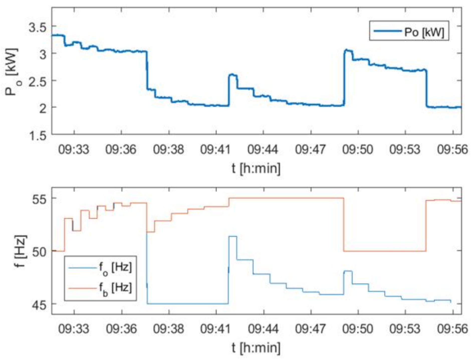
The algorithm was tested in real conditions on a 100 mm diameter electromagnetic mill. An example of the recorded results is presented in Figure 19. Within the period of 5 min, the desired magnetic induction was increased by 5 mT (the starting value was 100 mT). In the first period, both the basic and output frequencies were equal. The succeeding steps show a reduction of the active power starting from 3.3 kW and finishing at 3 kW. When the required induction increased in the second period of the experiment, another active constraint was found, which resulted in different values of frequencies (the output frequency reached its limit). However, finally, the active power was reduced to 2 kW. It is interesting to notice that even when the required magnetic strength increased, active power was reduced. Obviously, the next increase (in 4th period of experiment) caused an increase of the active power.
5. Conclusions
The methodology of batch grinding in EMM has proven to be effective for the purpose of comparing different process parameters. It allows us to contrast the results without influencing external disturbances. Moreover, it allows for the continuous process parametrization and estimation of energetic efficiency. Several issues were noticed, however, mainly for short processing times. The results obtained for larger graining media or higher densities should be studied further, primarily with respect to continuous process in grinding and classification circuits. The methodology for compete circuit parametrization based on the batch experimental results is the natural goal.
Wet grinding technology in EMM has been showed to be more effective than the dry technology. When the energy required for the pneumatic and hydraulic transport system is compared, that difference is even clearer. Research on dry grinding is, however, necessary, because some material can only be grinded in dry technology. Comparison of dry grinding results between EMM and other standard solutions showed certain advantages of such a processing method. Further research on product parameters is, however, necessary. Estimation of the processing time required for a specific size of the product grains and sharp edges is one of the challenging problems. Product grains reactivity, i.e., floatability of copper ore based on EMM grinding process parameters is another important issue. Influence of the processed material moisture on the grinding process in EMM will be studied further as well, also for the moisture control purposes. The EMM can be viewed as very competitive in relation to other milling solutions and at the same time it delivers a wide range of research problems.
Acknowledgments
The work has been supported by the Polish Ministry of Science and Higher Education, grant of Institute of Automatic Control, Silesian University of Technology. The research reported in this paper was also co-financed by the National Centre for Research and Development, Poland, under Applied Research Program, project No. PBS3/B3/28/2015.
Author Contributions
S.O., Z.O., D.F. and M.P. conceived and designed the grinding and classification circuits, S.O. M.W.-G. and D.F. conceived and performed the batch experiments, M.W.-G. and D.F. prepared the samples and performed laboratory analysis, S.O. designed the factors and indicators and performed data analysis, Z.O. designed and solved the energy optimization problem, M.P. supervised the research, S.O., M.W.-G. and Z.O. wrote the paper.
Conflicts of Interest
The authors declare no conflict of interest.
References
- Blaschke, S. Mechanical Processing of Minerals, Part I; Wydawnictwo Śląsk: Katowice, Poland, 1982. (In Polish) [Google Scholar]
- Fuerstenau, D.W.; Abouzeid, A.-Z.M. The energy efficiency of ball milling in comminution. Int. J. Miner. Process. 2002, 67, 161–185. [Google Scholar] [CrossRef]
- Gawenda, T. Issues of crushing devices selection for mineral aggregates production circuits. Górnictwo i Geoinżynieria 2010, 34, 195–209. (In Polish) [Google Scholar]
- Malewski, J. Mineral Processing. Principles of Comminution and Classification; Wydawnictwo Politechniki Wrocławskiej: Wrocław, Poland, 1981. (In Polish) [Google Scholar]
- Laskowski, J.; Łuszczkiewicz, A. Mineral Processing. Enrichment of Mineral Resources; Skrypt Politechniki Wrocławskiej: Wrocław, Poland, 1989. (In Polish) [Google Scholar]
- Wills, B.; Napier-Munn, T. Mineral Processing Technology, 7th ed.; Pergamon Press: Oxford, UK, 2006; pp. 146–186. [Google Scholar]
- Clermont, B.; De Haas, B. Optimization of mill performance by using online ball and pulp measurements. J. S. Afr. Inst. Min. Metall. 2010, 110, 133–140. [Google Scholar]
- Wang, Y.M.; Forssberg, E. New Milling Technology; Technical Report; MinFo: Stockholm, Sweden, 2001. [Google Scholar]
- Mular, A.L.; Doug, N.H.; Derek, J.B. Mineral Processing Plant Design. Practice and Control Proceedings; SME: Chicago, IL, USA, 2002; pp. 537–669. [Google Scholar]
- Bruckard, W.J.; Sparrow, G.J.; Woodcock, J.T. A Review of the Effects of the Grinding Environment on the Flotation of Copper Sulphides. Int. J. Miner. Process. 2011, 100, 1–13. [Google Scholar] [CrossRef]
- Herbst, J.A.; Nordell, L.K. Emergence of HFS as a design tool in mineral processing. In Proceedings of the Mineral Processing Plant Design, Practice, and Control, Vancouver, BC, Canada, 20–24 October 2002; Mular, A.L., Halbe, D.N., Barratt, D.J., Eds.; Society for Mining, Metallurgy, and Exploration: Chicago, IL, USA, 2002; pp. 495–506, ISBN 0-87335-223-8. [Google Scholar]
- Morrison, R.D.; Richardson, J.M. JKSimMet: A simulator for analysis, optimization and design of comminution circuit. In Proceedings of the Mineral Processing Plant Design, Practice, and Control, Vancouver, BC, Canada, 20–24 October 2002; Mular, A.L., Halbe, D.N., Barratt, D.J., Eds.; Society for Mining, Metallurgy, and Exploration: Chicago, IL, USA, 2002; pp. 442–460, ISBN 0-87335-223-8. [Google Scholar]
- Wołosiewicz-Głąb, M.; Ogonowski, S.; Foszcz, D. Construction of the electromagnetic mill with the grinding system, classification of crushed minerals and the control system. IFAC-PapersOnLine 2016, 49, 67–71. [Google Scholar] [CrossRef]
- Wołosiewicz-Głąb, M.; Foszcz, D.; Ogonowski, S. Design of the electromagnetic mill and the air stream ratio model. IFAC-PapersOnLine 2017, 50, 14964–14969. [Google Scholar] [CrossRef]
- Pawełczyk, M.; Ogonowski, Z.; Ogonowski, S.; Foszcz, D.; Saramak, D.; Gawenda, T.; Krawczykowski, D. Method for Dry Grinding in Electromagnetic Mill. Patent PL413041, 6 July 2015. [Google Scholar]
- Ogonowski, Z.; Ogonowski, S. Estimation problems of pneumatic transport system for electromagnetic grinding. In Proceedings of the 22nd International Conference on Methods and Models in Automation and Robotics (MMAR 2017), Międzyzdroje, Poland, 28–31 August 2017. [Google Scholar] [CrossRef]
- Ogonowski, S.; Ogonowski, Z.; Pawelczyk, M. Model of the air stream ratio for an electromagnetic mill control system. In Proceedings of the 21st International Conference on Methods and Models in Automation and Robotics (MMAR 2016), Międzyzdroje, Poland, 29 August–1 September 2016; pp. 901–906. [Google Scholar] [CrossRef]
- Krauze, O.; Pawełczyk, M. Modelling dynamics of strongly coupled air paths in pneumatic transport system for milling product. In Proceedings of the 22nd International Conference on Methods and Models in Automation and Robotics (MMAR 2017), Międzyzdroje, Poland, 28–31 August 2017. [Google Scholar] [CrossRef]
- Wolosiewicz-Glab, M.; Ogonowski, S.; Foszcz, D.; Gawenda, T. Assessment of classification with variable air flow for inertial classifier in dry grinding circuit with electromagnetic mill using partition curves. Physicochem. Probl. Miner. Process. 2018, 54, 440–447. [Google Scholar] [CrossRef]
- Buchczik, D.; Wegehaupt, J.; Krauze, O. Indirect measurements of milling product quality in the classification system of electromagnetic mill. In Proceedings of the 22nd International Conference on Methods and Models in Automation and Robotics (MMAR 2017), Międzyzdroje, Poland, 28–31 August 2017. [Google Scholar] [CrossRef]
- Ogonowski, S.; Ogonowski, Z.; Swierzy, M.; Pawelczyk, M. Control System of Electromagnetic Mill Load. In Proceedings of the 2017 25th International Conference on Systems Engineering (ICSEng), Las Vegas, NV, USA, 22–24 August 2017; pp. 69–76. [Google Scholar] [CrossRef]
- Ogonowski, S.; Ogonowski, Z.; Swierzy, M. Power optimizing control of grinding process in electromagnetic mill. In Proceedings of the 2017 21st International Conference on Process Control (PC 2017), Strbske Pleso, Slovakia, 6–9 June 2017; pp. 370–375. [Google Scholar] [CrossRef]
- Ogonowski, S.; Ogonowski, Z.; Pawelczyk, M. Multi-objective and multi-rate control of the grinding and classification circuit with electromagnetic mill. Appl. Sci. 2018, 8, 506. [Google Scholar] [CrossRef]
- Sławiński, K.; Gandor, M.; Knaś, K.; Balt, B.; Nowak, W. Electromagnetic mill and its application for coal drying process. Rynek Energii 2014, 1, 140–150. [Google Scholar]
- Lynch, A.J. Mineral Crushing and Grinding Circuits: Their Simulation, Optimization, Design and Control; Elsevier Scientific: New York City, NY, USA, 1977; ISBN 978-0444415288. [Google Scholar]
- Krawczykowski, D. Application of Diffraction Laser Analysis to Monitor Granulation of Copper Ores Processing Products. Inżynieria Mineralna 2017, 1, 233–240. (In Polish) [Google Scholar]
- Kincaid, D.; Cheney, W. Numerical Analysis. Mathematics of Scientific Computing; Brooks/Cole Publishing: Pacific Grove, CA, USA, 2002; ISBN 0-534-13014-3. [Google Scholar]
- International Organization for Standardization. Particle Size Analysis—Laser Diffraction Methods; ISO13320; International Organization for Standardization: Geneva, Switzerland, 2009. [Google Scholar]
- Wegehaupt, J.; Buchczik, D.; Krauze, O. Preliminary studies on modelling the drying process in product classification and separation path in an electromagnetic mill installation. In Proceedings of the 22nd International Conference on Methods and Models in Automation and Robotics (MMAR 2017), Międzyzdroje, Poland, 28–31 August 2017. [Google Scholar] [CrossRef]
Figure 1.
Modes of size reduction: a—two-sided compression, b—shearing, c—one-sided impact.

Figure 2.
Construction of electromagnetic mill: (a) electromagnets; (b) the mill with the cover and supply cabinet; (c) working chamber with the grinding media during operation.
Figure 2.
Construction of electromagnetic mill: (a) electromagnets; (b) the mill with the cover and supply cabinet; (c) working chamber with the grinding media during operation.

Figure 3.
Dry grinding and classification circuit: (a) Idea of the circuit: 1-feed stream, 2-mill working chamber, 3-working area with ferromagnetic rods, 4-main transport air stream, 5-mills output stream, 6-recycle material stream, 7-recycle material with transport air stream, 8-final product stream, 9-coarse ungrindable particles stream, 10-additional air stream for the classifier, 11–13-air dumping flaps; (b) Exemplary installation with the D200 electromagnetic mill (EMM).
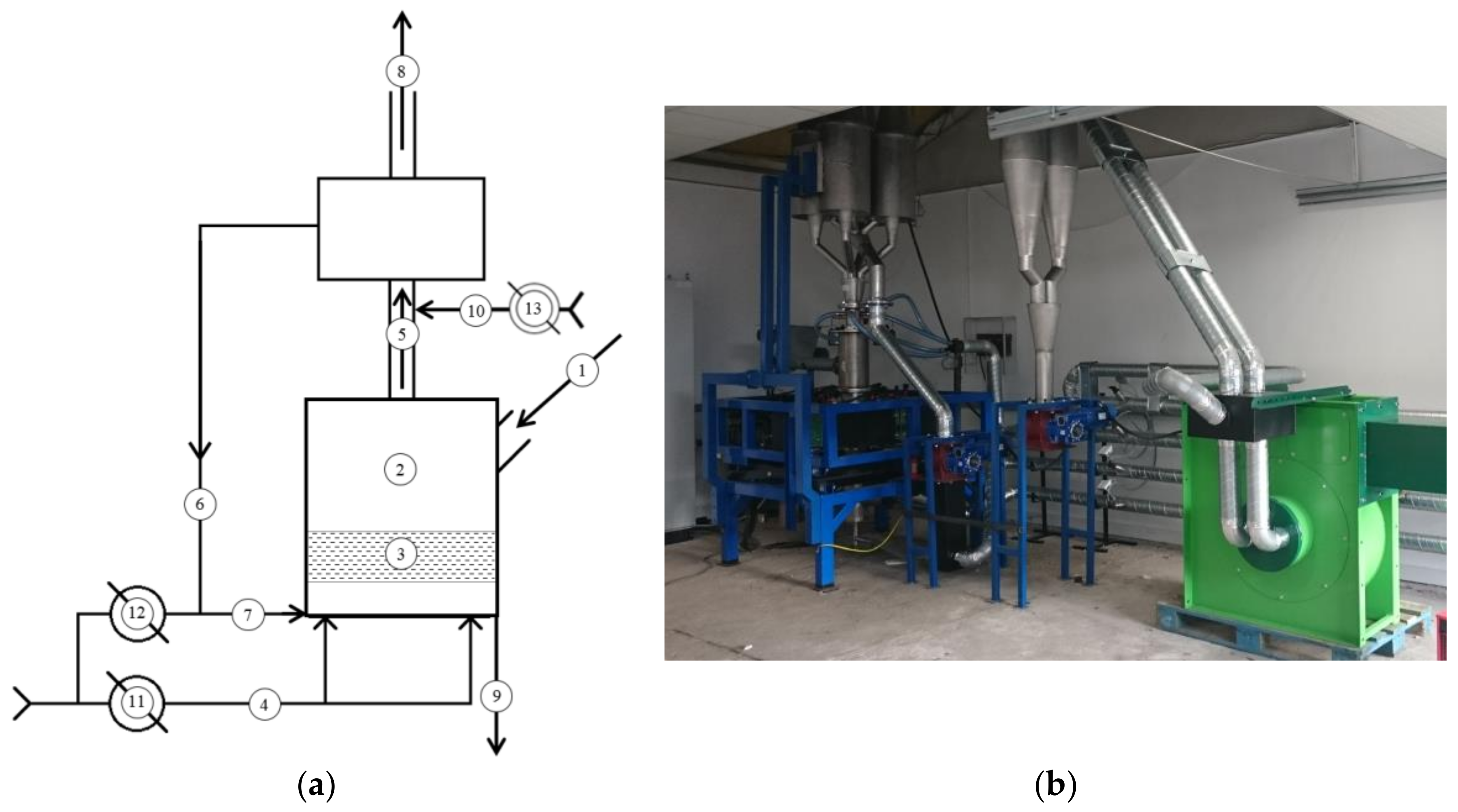
Figure 4.
3D model of the dry grinding and classification circuit with D200 EMM by ELTRAF.

Figure 5.
Open wet grinding circuit with EMM (a) and close wet grinding circuit with recycle of coarse particles using hydrocyclone (b).
Figure 5.
Open wet grinding circuit with EMM (a) and close wet grinding circuit with recycle of coarse particles using hydrocyclone (b).

Figure 6.
Batch working chamber for EMM: (a) Empty, open chamber; (b) Closed chamber in working position inside EMM.
Figure 6.
Batch working chamber for EMM: (a) Empty, open chamber; (b) Closed chamber in working position inside EMM.

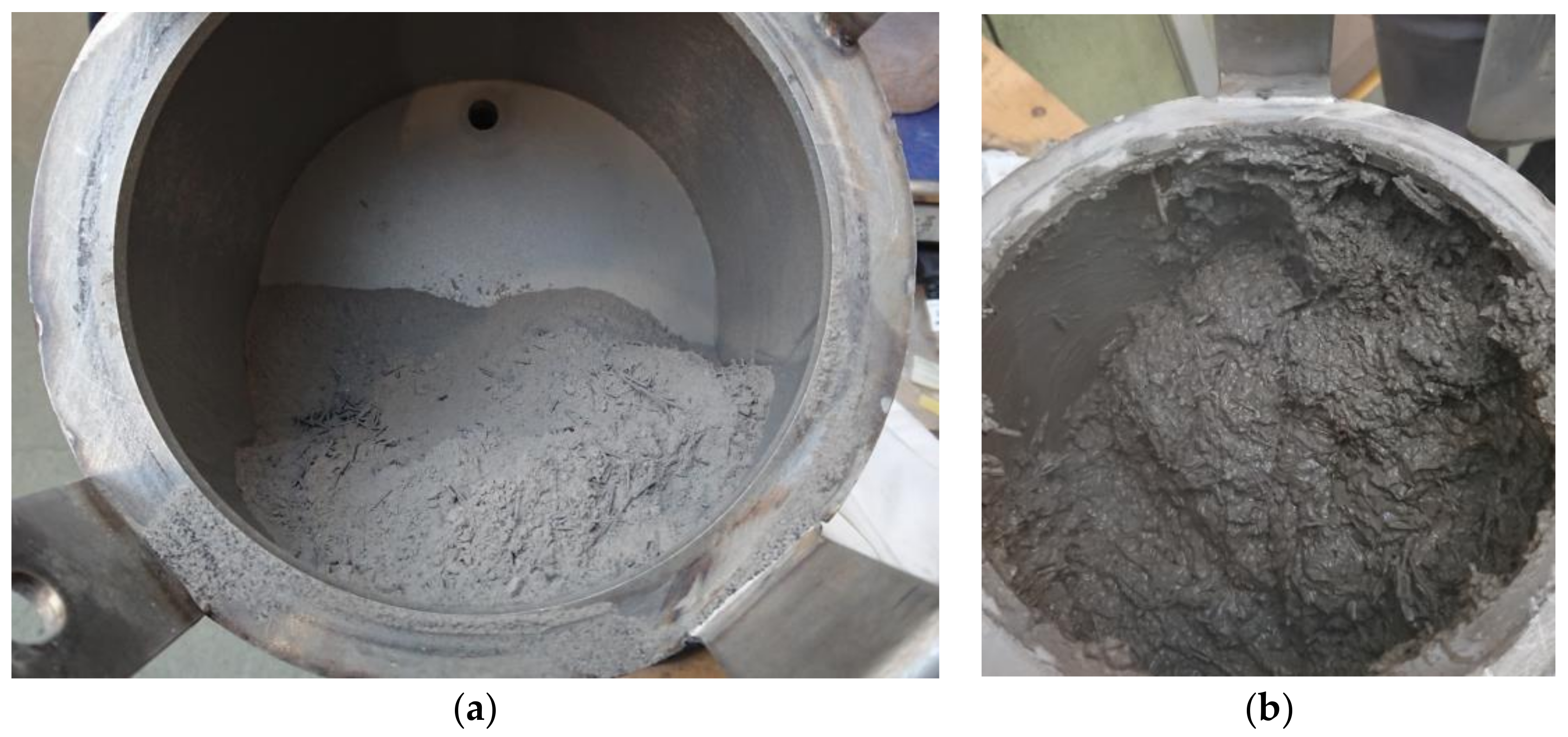
Figure 7.
Working chamber during grinding experiments: (a) dry grinding; (b) wet grinding.

Figure 8.
Example of surface areas below the cumulative volume curves: FAREA (blues) and PAREA (orange).
Figure 8.
Example of surface areas below the cumulative volume curves: FAREA (blues) and PAREA (orange).
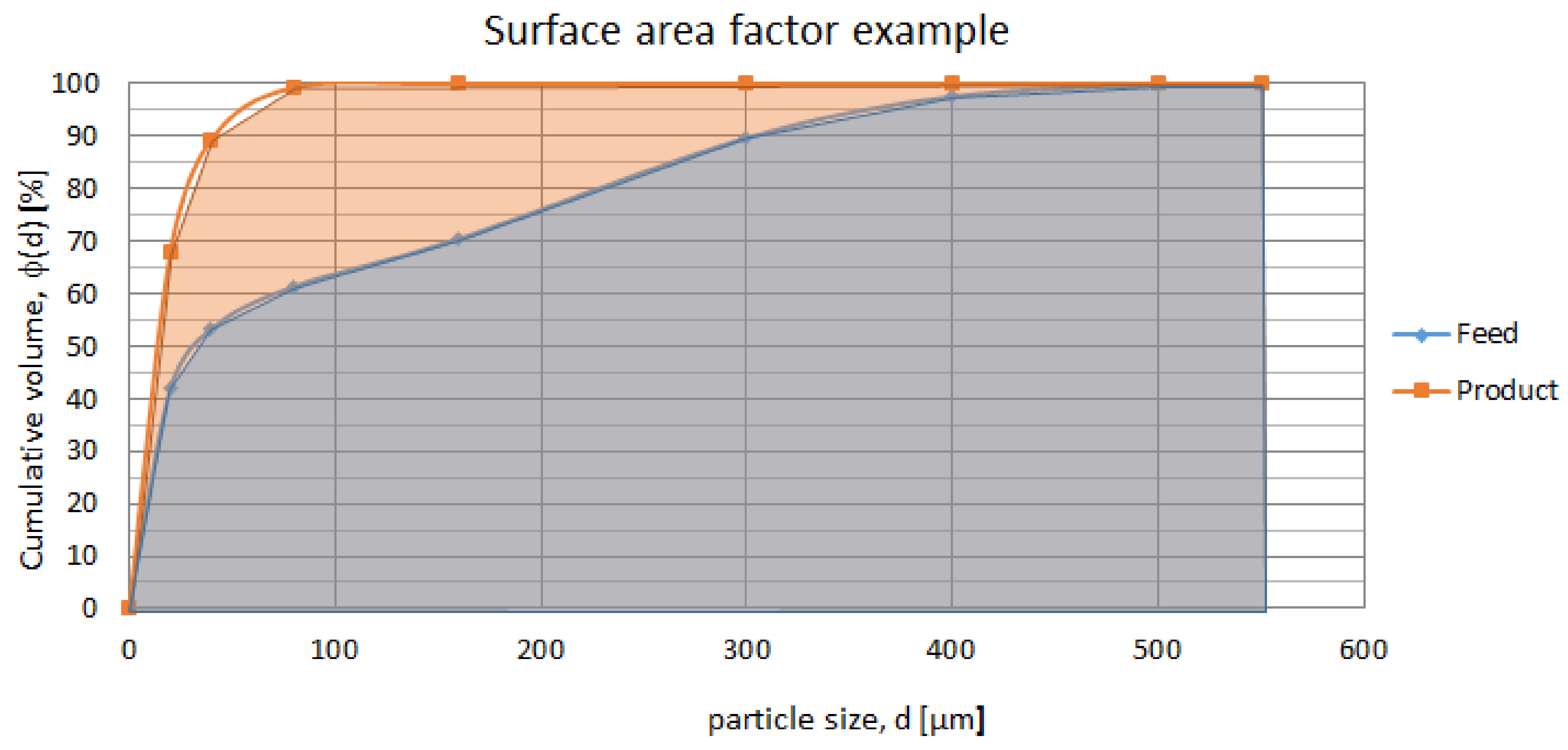
Figure 9.
Cumulative volume distribution of grains with size lower then 50 µm in the dry grinding product.
Figure 9.
Cumulative volume distribution of grains with size lower then 50 µm in the dry grinding product.

Figure 10.
Comparison of d80 size in the product dry grinding.
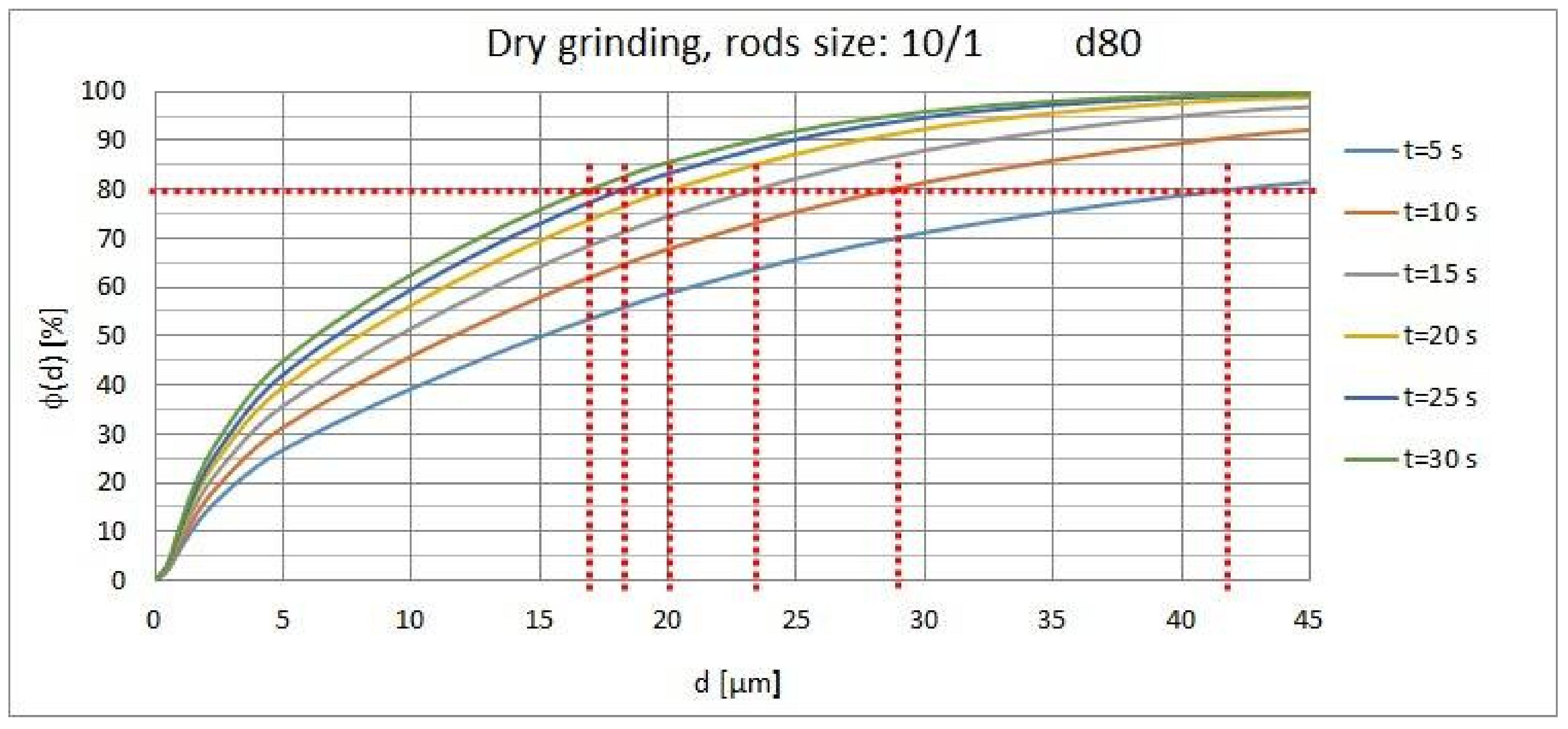
Figure 11.
Comparison of SR factors for dry grinding with 10/1 mm rods.

Figure 12.
Comparison of SNDIFF factor for wet grinding with 10/1 mm rods.

Figure 13.
Comparison of cumulative volume curves for dry grinding with different rods: (a) 10 s; (b) 5 s and (c) 15 s of processing time.
Figure 13.
Comparison of cumulative volume curves for dry grinding with different rods: (a) 10 s; (b) 5 s and (c) 15 s of processing time.

Figure 14.
Comparison of SR factors for wet grinding with 10/1 mm rods and 1600 kg/m3 density.

Figure 15.
Comparison of SNDIFF factor for wet grinding with 10/1 mm rods and 1600 kg/m3 density.

Figure 16.
Comparison of cumulative volume curves for the dry and wet grinding process (t = 5 s).

Figure 17.
Comparison of cumulative volume curves for dry and wet grinding process (t = 10 s).

Figure 18.
Example of measurements, model and constraints (a) of active power optimization and final feasible region (b) for the electromagnetic mill of 100 mm working chamber diameter (EMM D100).
Figure 18.
Example of measurements, model and constraints (a) of active power optimization and final feasible region (b) for the electromagnetic mill of 100 mm working chamber diameter (EMM D100).
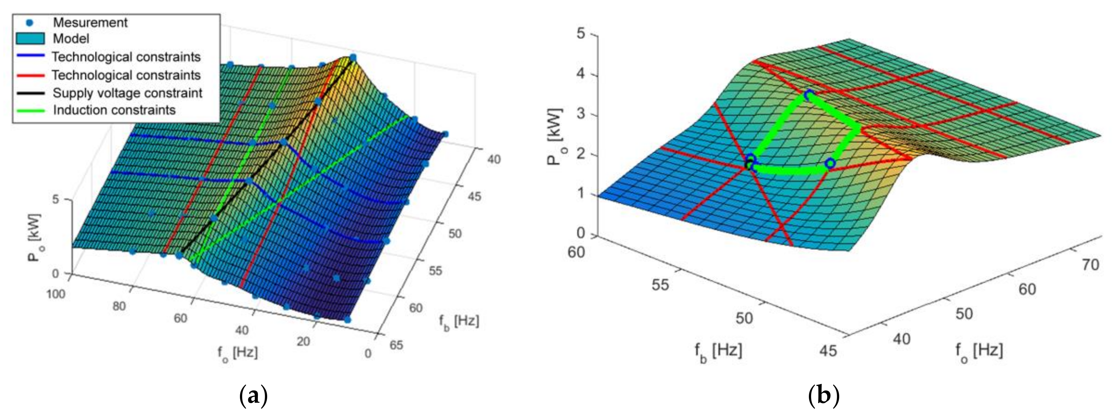
Figure 19.
Example of optimization experiment (on-line optimization) for EMM D100. Symbols are the same as in Figure 18.
Figure 19.
Example of optimization experiment (on-line optimization) for EMM D100. Symbols are the same as in Figure 18.


Table 1.
Experiments’ parameters for copper ore dry grinding in EMM, material mass 500 g (4% of WCV) and grinding media mass 1500 g (9% of WCV).
Table 1.
Experiments’ parameters for copper ore dry grinding in EMM, material mass 500 g (4% of WCV) and grinding media mass 1500 g (9% of WCV).
| Sample No. | Processing Time (s) | Rods Size l (mm)/d (mm) | Sample No. | Processing Time (s) | Rods Size l (mm)/d (mm) |
|---|---|---|---|---|---|
| 1 | 5 | 10/1 | 13 | 5 | 12/2 |
| 2 | 10 | 10/1 | 14 | 10 | 12/2 |
| 3 | 15 | 10/1 | 15 | 15 | 12/2 |
| 4 | 20 | 10/1 | 16 | 20 | 12/2 |
| 5 | 25 | 10/1 | 17 | 25 | 12/2 |
| 6 | 30 | 10/1 | 18 | 30 | 12/2 |
| 7 | 5 | 12/1.5 | 19 | 5 | mixture |
| 8 | 10 | 12/1.5 | 20 | 10 | mixture |
| 9 | 15 | 12/1.5 | 21 | 15 | mixture |
| 10 | 20 | 12/1.5 | 22 | 20 | mixture |
| 11 | 25 | 12/1.5 | 23 | 25 | mixture |
| 12 | 30 | 12/1.5 | 24 | 30 | mixture |
Table 2.
Experimental parameters for copper ore wet grinding in EMM, solids mass 470 g and grinding media (10/1 type) mass 1500 g (9% of WCV).
Table 2.
Experimental parameters for copper ore wet grinding in EMM, solids mass 470 g and grinding media (10/1 type) mass 1500 g (9% of WCV).
| Sample No. | Pulp Density (kg/m3) | Sample Volume (mL) | Water Volume (mL) | Sample WCV Ratio (%) | Processing Time (s) |
|---|---|---|---|---|---|
| 1 | 1600 | 506 | 330 | 10.1 | 5 |
| 2 | 1600 | 506 | 330 | 10.1 | 10 |
| 3 | 1600 | 506 | 330 | 10.1 | 15 |
| 4 | 1700 | 430 | 253 | 8.6 | 5 |
| 5 | 1700 | 430 | 253 | 8.6 | 10 |
| 6 | 1700 | 430 | 253 | 8.6 | 15 |
| 7 | 1800 | 375 | 198 | 7.5 | 5 |
| 8 | 1800 | 375 | 198 | 7.5 | 10 |
| 9 | 1800 | 375 | 198 | 7.5 | 15 |
Table 3.
Comparison of grinding effectiveness factors for dry grinding with 10/1 mm rods.
| Time (s) | Energy Consumption (kWh) | Specific Energy (kWh/t) | SDIFF ± RSD | SNDIFF ± RSD (%) | SR50 ± RSD | SR80 ± RSD |
|---|---|---|---|---|---|---|
| 5 | 0.025 | 50 | 7512.86 ± 744.42 | 16.84 ± 1.75 | 2.08 ± 0.31 | 5.46 ± 0.58 |
| 10 | 0.05 | 100 | 8676.44 ± 756.05 | 19.45 ± 1.79 | 2.71 ± 0.41 | 7.98 ± 0.85 |
| 15 | 0.075 | 150 | 9017.59 ± 759.47 | 20.21 ± 1.80 | 3.32 ± 0.50 | 9.78 ± 1.04 |
| 20 | 0.1 | 200 | 9217.12 ± 761.46 | 20.66 ± 1.81 | 3.96 ± 0.59 | 11.38 ± 1.22 |
| 25 | 0.125 | 250 | 9340.27 ± 762.69 | 20.93 ± 1.81 | 4.46 ± 0.67 | 12.58 ± 1.34 |
| 30 | 0.15 | 300 | 9420.22 ± 763.49 | 21.11 ± 1.82 | 5.04 ± 0.76 | 13.53 ± 1.45 |
Table 4.
Comparison of grinding effectiveness factors for wet grinding with 10/1 mm rods and 1600 kg/m3 density.
Table 4.
Comparison of grinding effectiveness factors for wet grinding with 10/1 mm rods and 1600 kg/m3 density.
| Time (s) | Energy Consumption (kWh) | Specific Energy (kWh/t) | SDIFF ± RSD | SNDIFF ± RSD (%) | SR50 ± RSD | SR80 ± RSD |
|---|---|---|---|---|---|---|
| 5 | 0.025 | 53 | 6584.10 ± 735.13 | 14.76 ± 1.72 | 1.76 ± 0.26 | 3.62 ± 0.39 |
| 10 | 0.05 | 106 | 8926.39 ± 758.55 | 20.01 ± 1.80 | 3.05 ± 0.46 | 9.08 ± 0.97 |
| 15 | 0.075 | 159 | 9100.61 ± 760.30 | 20.4 ± 1.81 | 3.51 ± 0.53 | 10.10 ± 1.08 |
© 2018 by the authors. Licensee MDPI, Basel, Switzerland. This article is an open access article distributed under the terms and conditions of the Creative Commons Attribution (CC BY) license (http://creativecommons.org/licenses/by/4.0/).
Share and Cite
MDPI and ACS Style
Ogonowski, S.; Wołosiewicz-Głąb, M.; Ogonowski, Z.; Foszcz, D.; Pawełczyk, M. Comparison of Wet and Dry Grinding in Electromagnetic Mill. Minerals 2018, 8, 138. https://doi.org/10.3390/min8040138
AMA Style
Ogonowski S, Wołosiewicz-Głąb M, Ogonowski Z, Foszcz D, Pawełczyk M. Comparison of Wet and Dry Grinding in Electromagnetic Mill. Minerals. 2018; 8(4):138. https://doi.org/10.3390/min8040138
Chicago/Turabian StyleOgonowski, Szymon, Marta Wołosiewicz-Głąb, Zbigniew Ogonowski, Dariusz Foszcz, and Marek Pawełczyk. 2018. "Comparison of Wet and Dry Grinding in Electromagnetic Mill" Minerals 8, no. 4: 138. https://doi.org/10.3390/min8040138
Note that from the first issue of 2016, this journal uses article numbers instead of page numbers. See further details here.