Modeling the Effect of Composition and Temperature on the Conductivity of Synthetic Copper Electrorefining Electrolyte

Abstract

The physico-chemical properties of the copper electrolyte significantly affect the energy consumption of the electrorefining process and the quality of the cathode product. Favorable conditions for electrorefining processes are typically achieved by keeping both the electrolyte conductivity and diffusion coefficient of Cu(II) high, while ensuring low electrolyte viscosity. In this work the conductivity of the copper electrorefining electrolyte was investigated as a function of temperature (50–70 °C) and concentrations of copper (Cu(II), 40–60 g/L), nickel (Ni(II), 0–20 g/L), arsenic (As(III), 0–30 g/L) and sulfuric acid (160–220 g/L). In total 165 different combinations of these factors were studied. The results were treated using factorial analysis, and as a result, four electrolyte conductivity models were built up. Models were constructed both with and without arsenic as the presence of As(III) appeared to cause non-linearity in some factor effects and thus impacted the conductivity in more complex ways than previously detailed in literature. In all models the combined effect of factors was shown to be minor when compared to the effect of single factors. Conductivity was shown to increase when copper, nickel and arsenic concentrations were decreased and increase with increased temperature and acidity. Moreover, the arsenic concentration was shown to decrease the level of conductivity more than previously suggested in the literature.

1. Introduction

Copper electrorefining is the most common method for producing high-purity copper [1]. The first refinery (Pembrey Copper Works) was established in 1869 following the first patent for commercial electrorefining developed by James Elkington in 1865 [2,3]. Since then, the process has been developed further as the result of both research and improved industrial practices [2]. In the copper electrorefining process, copper is dissolved from impure copper anodes into the electrolyte bath and then subsequently deposited on to cathodes as high-purity copper [4].

Industrial copper refining electrolytes mainly consist of water, copper sulfate, sulfuric acid, with additional leveling/grain-refining agents—to obtain smoother and denser cathode deposits—and process impurities [4,5]. These impurities commonly consist of nickel, arsenic and iron, along with smaller amounts of bismuth, antimony and chloride that dissolve into the electrolyte from the anode.

The physico-chemical properties of the copper electrolyte significantly affect the yield of cathodic copper in the electrorefining process and include four main physico-chemical properties: conductivity, density, viscosity and the diffusion coefficient of the cupric ion (Cu(II)) [5,6,7,8,9,10,11]. The best yield of copper can be obtained by keeping the electrolyte viscosity low [5] while ensuring a high diffusion coefficient [7] and electrical conductivity [5]. These properties of the copper electrolyte are strongly influenced by composition and temperature: Increased temperature, for example, lowers electrolyte density and viscosity [6] while enhancing the rate of chemical reactions [4]. On the other hand, a too-high temperature results in unnecessary energy costs and excessive electrolyte bath evaporation [4]. In contrast, an electrolyte composition with a high concentration of Cu(II), Ni(II) and sulfuric acid makes the electrolyte denser and more viscous [6,12]. An increase in viscosity decreases the diffusion coefficient of Cu(II) but a high concentration of Cu(II) also increases the limiting current density [7], giving the possibility for a higher deposition rate. Moreover, an increase in the concentration of sulfuric acid leads to enhanced conductivity [5,6,7]. As a result, it is important to thoroughly determine the effects of these parameters in order to optimize the yield of cathode copper.

Conductivity is an important solution property [13] as it affects the electrical energy consumption of the electrorefining process [5,6]. Therefore, when optimizing the refining process by altering the temperature or composition, conductivity is a good value to be controlled either by measuring it or defining it with an applicable model.

The aim of this study is to construct accurate mathematical models for the conductivity, taking into account the effect of temperature as well as solution sulfuric acid and metal concentrations. Furthermore, a particular focus is also paid to the effect of typical impurities such as nickel and arsenic, originating from increasingly impure raw materials in addition to copper. The design of experiments is carried out with full factorial design by MODDE software (MKS Data Analytics Solutions, Malmö, Sweden) in order to build up a model that reflects copper electrorefining conductivity as a function of all the previously mentioned parameters.

2. Materials and Methods

Electrolytes were prepared from copper sulfate (CuSO₄·5H₂O, min. 98%, VWR Chemicals, Radnor, PA, USA), nickel sulfate (NiSO₄·6H₂O, min. 98%, VWR Chemicals), sulfuric acid (H₂SO₄, 95%–98%, Sigma-Aldrich, St. Louis, MO, USA), arsenic acid solution (from Boliden Harjavalta Copper electrorefinery, Harjavalta, Finland, containing [As] = 151,700 mg/L, [Cu] = 4794 mg/L, [Sb] = 3954 mg/L, [Ni] = 1688 mg/L, [Bi] = 6.2 mg/L, [Te] = 18.6 mg/L, [Pb] = 29 mg/L, [Ag] = 0.16 mg/L) and distilled water. Cu and Ni contents in arsenic acid were also taken into account when preparing the electrolytes.

Table 1. Parameters investigated affecting copper electrorefining electrolyte—factors ([Cu(II)], [H₂SO₄], [Ni(II)], [As(III)] and temperature, T) and their levels. Arsenic was adjusted by arsenic acid (Cu(II) and Ni(II) in acid taken into account).

Factor	Levels
Cu(II)	40; 50; 60	g/L
H2SO4	160; 180; 200; 220	g/L
Ni(II)	0; 10; 20	g/L
As(III)	0; 15; 30	g/L
T	50; 55; 60; 65; 70	°C

summarizes the experimental factors and solution parameters studied, 33 different solution parameter combinations were investigated at five different temperatures and in total 165 different combinations were studied. No extra additives such as glue, thiourea or chloride ions were used.

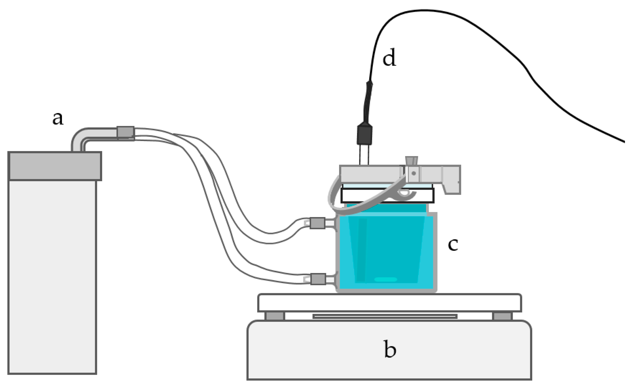
Conductivity measurements were carried out using a Knick Portamess^® 913 Cond conductivity meter produced by Knick Elektronische Messgeräte GmbH & Co. KG (Berlin, Germany). The meter was used with a four-electrode sensor (ZU 6985) which has glass/platinum measuring system and glass casing tube. All electrolytes were heated prior to measurement in a jacketed cell using a MGW Lauda MT/M3 circulating water bath (Figure 1) (LAUDA, Lauda-Königshofen, Germany). During the heating or between the measurements, the cell was completely covered and all the holes in the lid were plugged to prevent evaporation and consequently water loss. The electrolyte was stirred at 400 rpm using a magnetic stirrer.

Data analysis and experiment design were carried out using the Modeling and design tool MODDE 8 software (MKS Data Analytics Solutions, Malmö, Sweden) for design of experiments (DOE) and multivariate data analysis. The experiments were designed by defining factors, responses and levels of the factors using the full factorial design.

Prior to modeling, the raw data was explored and evaluated with scatter plots and histograms. The models were constructed according to the data and evaluated using regression analysis tools summary of fit, analysis of variance (ANOVA) and normal probability plot of residuals. In addition, the designs were checked to ensure a low enough condition number, i.e., the ratio of the minimum and maximum singular values of the factors. For a good design this value is less than 3, whereas in a bad design it is over 6 [14]. The effect of the changes in the models after refining was also determined by comparison of the change in value of the condition number.

In summary, the parameters that describe the model are goodness of fit (R²), goodness of prediction (Q²), model validity and reproducibility. Model validity is based on the lack of fit which is a statistical F-test where the model error is compared to replicate error [14]. In a valid model there is no lack of fit, and consequently the model validity is high. The reproducibility describes the variabilities in the replicates [14]. The models were refined to maximize these correlation coefficients as well as minimize the difference between the R² and Q² values [14]. In a good model the Q², the model validity and the reproducibility are larger than 0.5, 0.25 and 0.5, respectively [14]. In addition, the difference between the R² and Q² in a good model is less than 0.2–0.3 [14].

3. Results and Discussion

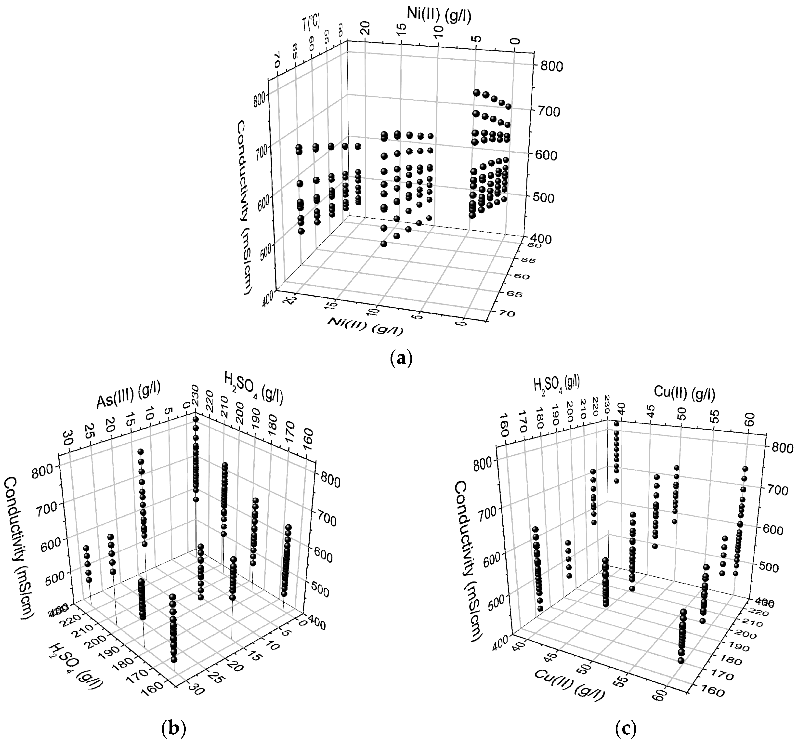
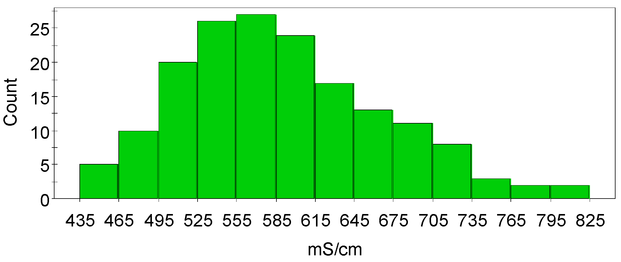
The histogram of the measured conductivity data is shown in Figure 2 and it can be seen that the histogram of the conductivity data is slightly skewed. The model validity and efficiency of data analysis are better when the data in the histogram plot is less skewed. Scatter plots of the raw data (Figure 3) showed both linearity and non-linearity which suggests that the relationship between some factors and the response might be curved, as well as the possibility that there may be interactions between the factors. Nevertheless, these scatter plots only give an approximate estimation of how the factors can influence the conductivity.

3.1. Conductivity Model 1—Untreated Data with Terms of [H₂SO₄]² and T²

In order to build up the first model that describes copper electrolyte conductivity, unscaled conductivity data was used. The model was constructed from the raw data despite the slightly skewed nature of the data (Figure 2).

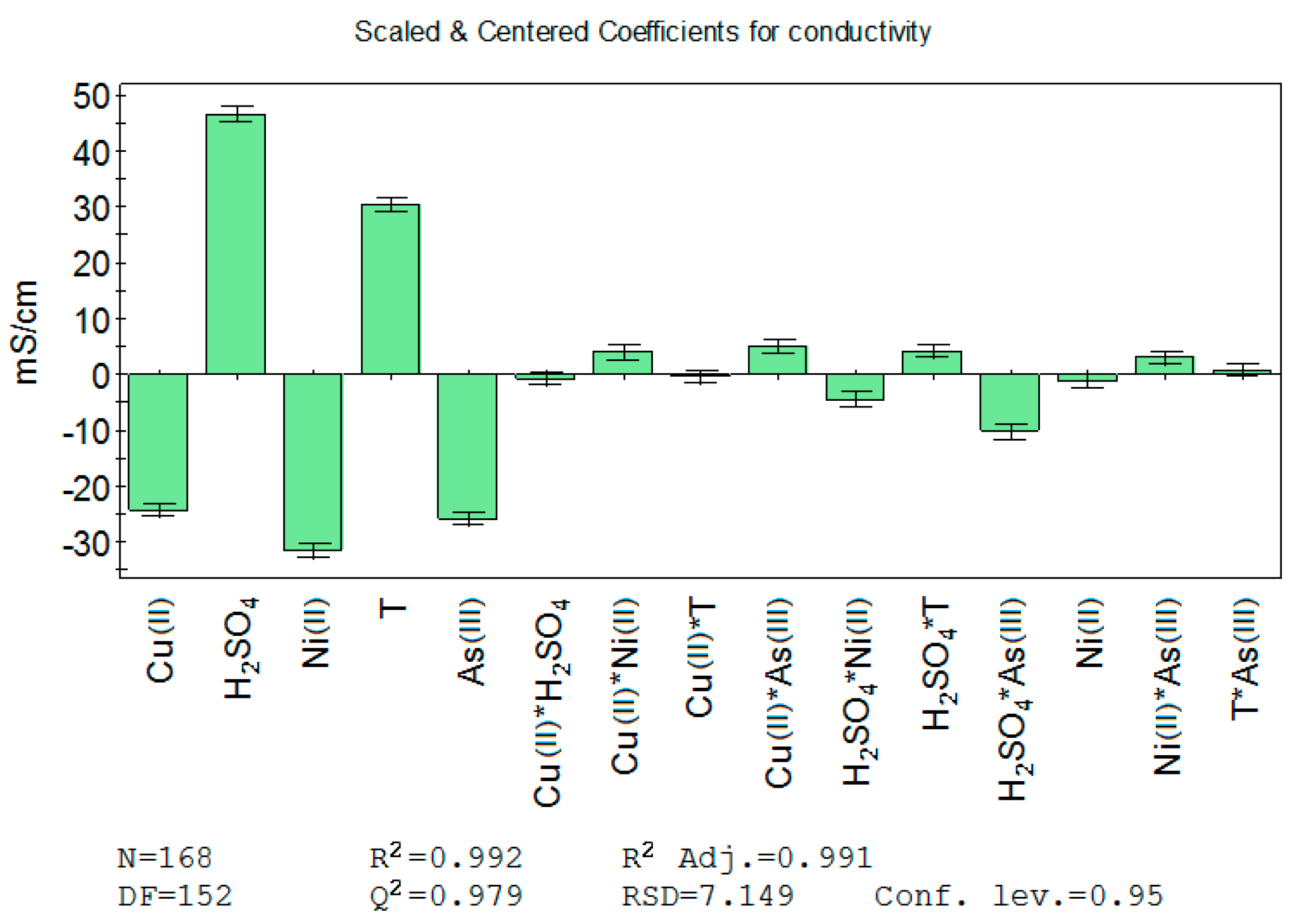
Coefficients for unrefined synthetic copper electrolyte conductivity (Model 1) are shown in Figure 4. It can be seen that in addition to the factors studied, the combined effect of two factors (product) is also investigated. Terms with a high p-value (probability value), in which the error bars extend over the zero line, need to be excluded from further analysis, e.g., the terms Cu(II)·H₂SO₄ and Cu(II)·T for Model 1. The summary of fit for Model 1 showed that the R², Q² and reproducibility were at a good level, but the model validity was found to be poor.

Model validity was improved by adding the squares of the terms to the model. Using squares [H₂SO₄]² and T², the irregularities of the normal probability plot could be reduced, although this was seen not to improve the model validity. Two result series (with a maximum amount of H₂SO₄, Cu(II) and Ni(II) as well as a maximum and medium amount of As(III)) were removed from the model, as it was suspected that these electrolytes were supersaturated and thus responsible for the skewness in the results.

These modifications resulted in a reasonable model validity as well as slightly higher R² and Q²; however, the condition number increased from 2.427 (with the unrefined data) to 4.517—slightly high but below 6—as a result of adding the terms [H₂SO₄]² and T². The model had no lack of fit in this phase and the summary of fit indicated that the model is valid (

Table 2. R², Q², model validity and reproducibility values of the models.

Model	1	2	3	4
R2	0.9978	0.9985	0.9972	0.9984
Q2	0.9876	0.9959	0.9661	0.9739
Model validity	0.3016	0.4598	0.2609	0.4194
Reproducibility	0.9997	0.9996	0.9996	0.9996

).

Equation (1) for conductivity Model 1 was compiled according to unscaled coefficients.

κ = 97.72 − 3.581 [Cu(II)] + 0.4736 [Ni(II)] + 0.596 [As(III)] + 2.945 [H₂SO₄] + 0.02396 [Cu(II)][Ni(II)] + 0.006713 [Cu(II)][As(III)] + 0.01219 [Ni(II)][As(III)] − 0.02297 [H₂SO₄][Ni(II)] − 0.02166 [H₂SO₄][As(III)] − 0.01899 [Ni(II)]T + 0.01768 T[As(III)] + 0.02754 [H₂SO₄]T + 2.743 T − 0.005364 [H₂SO₄]² − 0.02946 T²

(1)

where the concentrations are in g/dm³, T is in °C and κ is in mS/cm.

The equation has many terms, and all the effects of the factors are not fully seen in the equation coefficients. Nonetheless, factors with low p-values indicate that at least H₂SO₄ seems to have a combined effect with Ni(II), temperature and As(III). Data used for Model 1 indicated that Cu(II), Ni(II) and As(III) lower the conductivity of the electrolyte while temperature and H₂SO₄ increase it, which is in line with the literature [5,6].

3.2. Conductivity Model 2—Logarithmic Data with Terms of [H₂SO₄]² and T²

In order to avoid the skewness in Model 1 with untreated data, the second model was constructed using logarithmic values of conductivity and this resulted in a more normally distributed histogram. Terms with a high p-value were removed along with the two result series of the presumably supersaturated electrolytes determined from Model 1. As before, the term squares T² and [H₂SO₄]² were added to reduce the irregularities of the normal probability plot.

Equation (2) for the logarithm of the conductivity was compiled using unscaled coefficients. The strongest combined effects based on low p-values were shown to be with H₂SO₄∙T, H₂SO₄∙As(III) and T∙As(III); however, as with Model 1, the combined effects were minor compared to the single effects of factors.

log₁₀(κ) = 2.17388 − 0.0023479 [Cu(II)] − 0.0027733 [Ni(II)] − 0.00073729 [As(III)] + 0.0037764 [H₂SO₄] − 1.0649 × 10⁻⁵ [H₂SO₄][As(III)] + 2.1627 × 10⁻⁵ T[As(III)] + 8.8019 × 10⁻⁶ [H₂SO₄]T + 0.0051846 T − 6.9222 × 10⁻⁶ [H₂SO₄]² − 3.2506 × 10⁻⁵ T²,

(2)

Model 2 was regarded as reasonable and better with respect to Model 1, due to the improved model validity and Q² value, and Q² was almost equal to R² (Table 2). However, the condition number 4.456 was over 3, as was the condition number of Model 1, but not over 6, which would indicate a poor model. The condition number of this model was, however, lower than in Model 1.

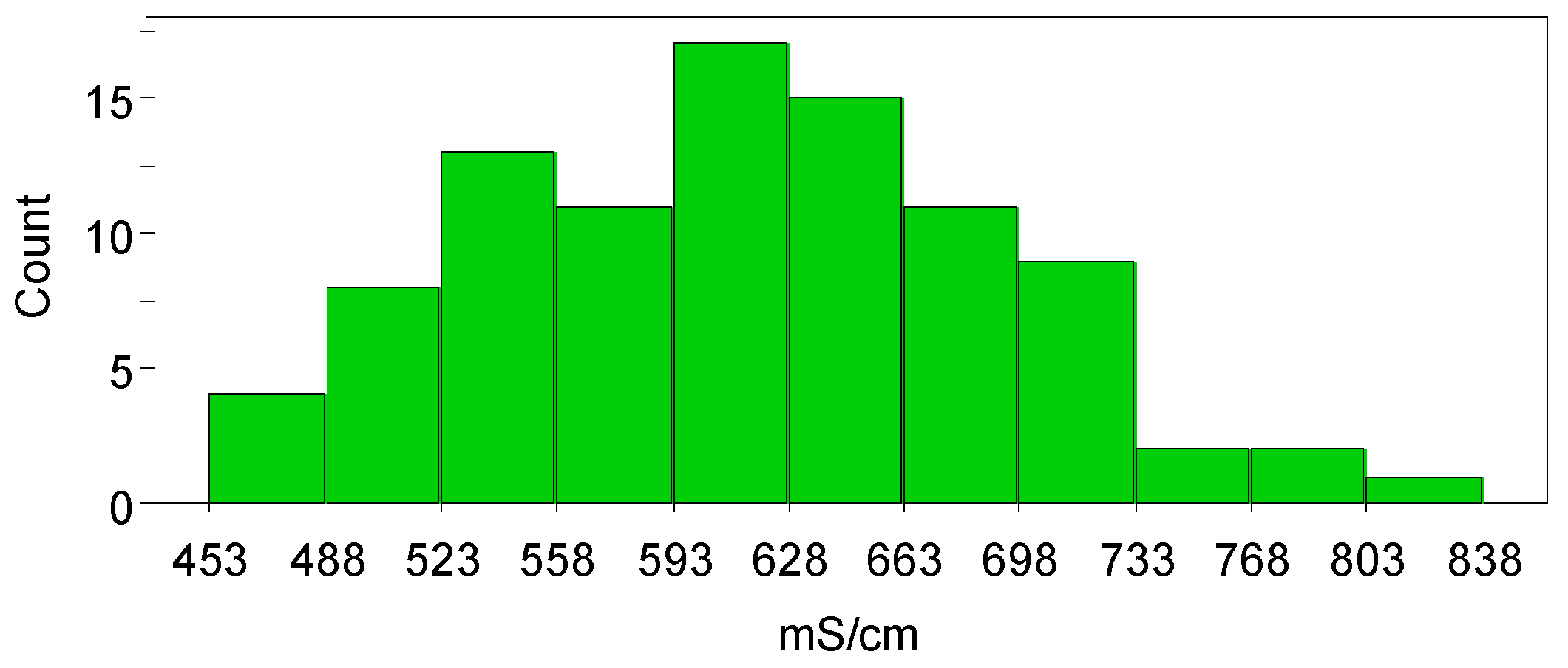
3.3. Conductivity Model 3—Untreated Data without Arsenic

The third conductivity model was constructed without the experiments containing arsenic and it was found out that the data was quite normally distributed (Figure 5). Scatter plots without arsenic did not vary remarkably from the corresponding plots with arsenic. Analogously, according to these plots, Cu(II) and Ni(II) were shown to lower the conductivity while temperature and H₂SO₄ were shown to increase it. This model, however, seems to have slightly better linearity in the relationships between the factors and the response than that observed in Models 1 and 2 which include the effect of As(III). Thus, As(III) seems to cause non-linearity in the model and also affects the conductivity in more complex ways than would be expected from the literature [5,6,10].

Model 3 was refined like Model 1 and compiled according to unscaled coefficients. The combined effect of H₂SO₄·Ni(II) and H₂SO₄·T was shown to affect the conductivity value; however, the single parameters (Cu(II), H₂SO₄, Ni(II) and T) had the biggest impact on conductivity. The sign (±) of an individual variable or combined effect of variables in the equation should not be interpreted individually, but as a combined effect of all variables that have an effect in the equation. Figure 6 shows the effect of Ni(II) and T on the conductivity according to Equation (3), which indicates increased conductivity with increased temperature and decreased nickel concentration. Model validity was good according to the summary of fit (Table 2).

κ = 307.9 − 1.583 [Cu(II)] + 2.737 [Ni(II)] + 1.285 [H₂SO₄] − 0.02776 [H₂SO₄][Ni(II)] − 0.008774 [Cu(II)][H₂SO₄] − 0.02087 [Ni(II)]T + 0.02919 [H₂SO₄]T − 1.17 T

(3)

3.4. Conductivity Model 4—Without Arsenic and with Terms of [H₂SO₄]² and T²

The fourth conductivity model was constructed without arsenic data and by adding extra terms of [H₂SO₄]² and T², identical to Models 1 and 2.

κ = 31.863 − 1.3594 [Cu(II)] + 1.835 [Ni(II)] + 2.9789 [H₂SO₄] − 0.022681 [H₂SO₄][Ni(II)] − 0.010403 [Cu(II)][H₂SO₄] − 0.021408 [Ni(II)]T + 0.02975 [H₂SO₄]T + 2.7297 T − 0.0044364 [H₂SO₄]² − 0.032787 T²

(4)

Both Models 3 and 4 were shown to be valid according to the summary of fit (Table 2), with model validity being better than that of Model 3. Conversely, the condition number, 1.375, was better in Model 3 when compared to the value of 4.322 in Model 4. In contrast, the condition number of the unrefined design was 1.838.

3.5. Summary of the Models

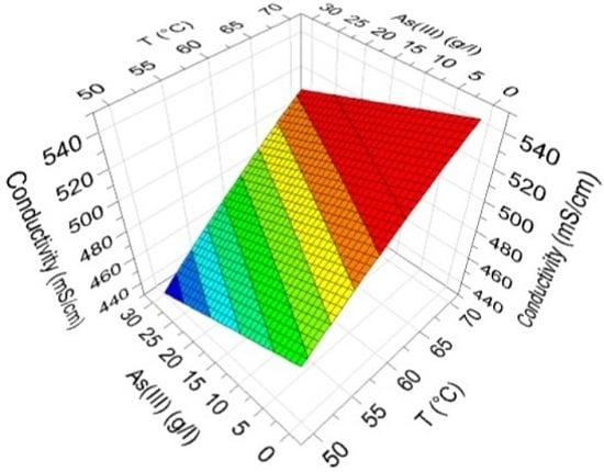
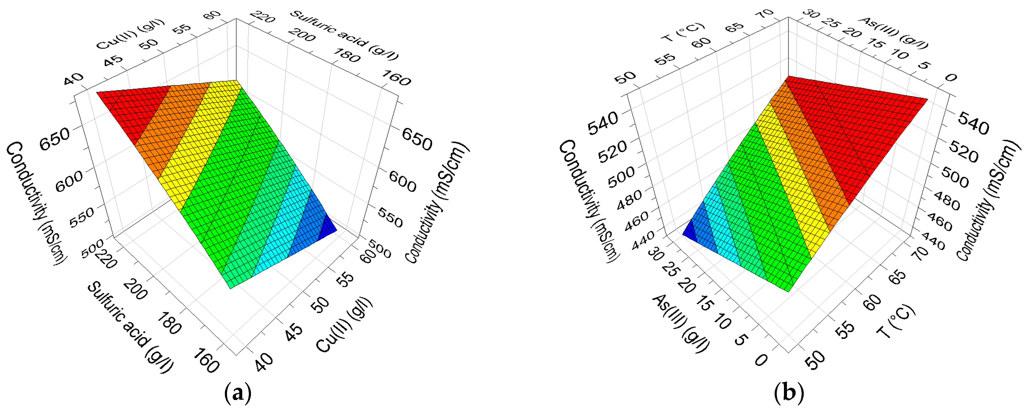
The defined Equations (1)–(4) are relatively complex due to the interactions of the factors, and thus the effects of the factors are impossible to directly see in the equations. The effects of Cu(II) and H₂SO₄ on electrolyte conductivity containing the median amount of As(III) and Ni(II) at medium temperature, defined with Model 1, are presented in Figure 7a. Analogously, the effects of As and temperature containing a high amount of Cu(II), a low amount of H₂SO₄ and a medium amount of Ni(II) are displayed in Figure 7b.

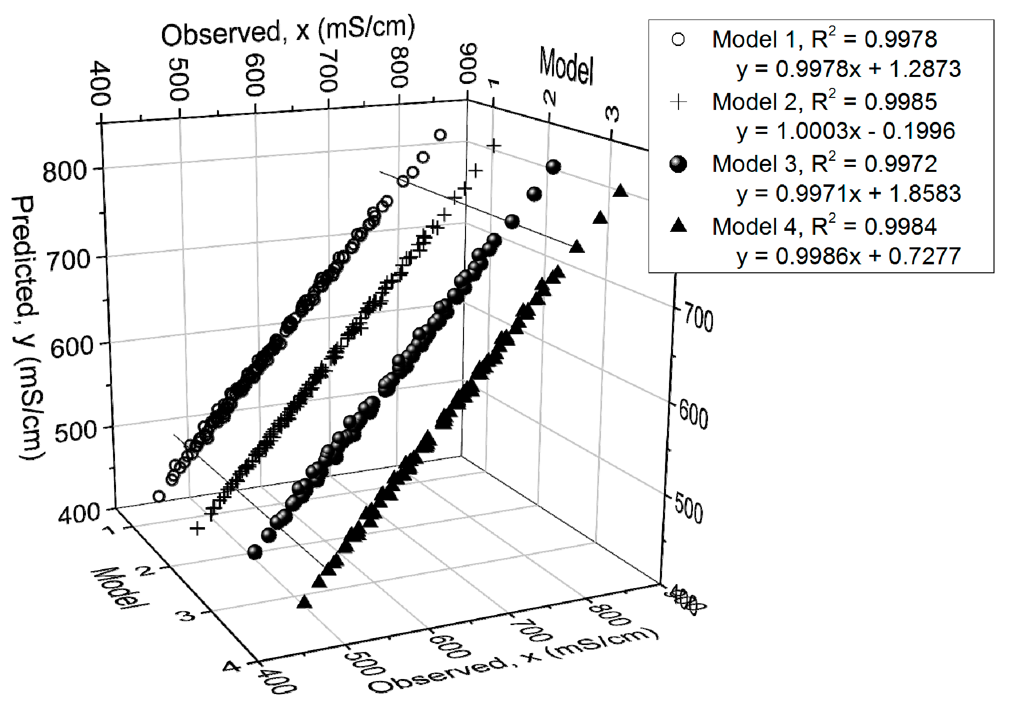
Figure 8 presents the measured and predicted electrolyte conductivity values. It can be seen that the models predict the data with high correlation, with R² varying from 0.9972 to 0.9985. In addition, the R², Q², model validity and reproducibility values of the models are presented in Table 2.

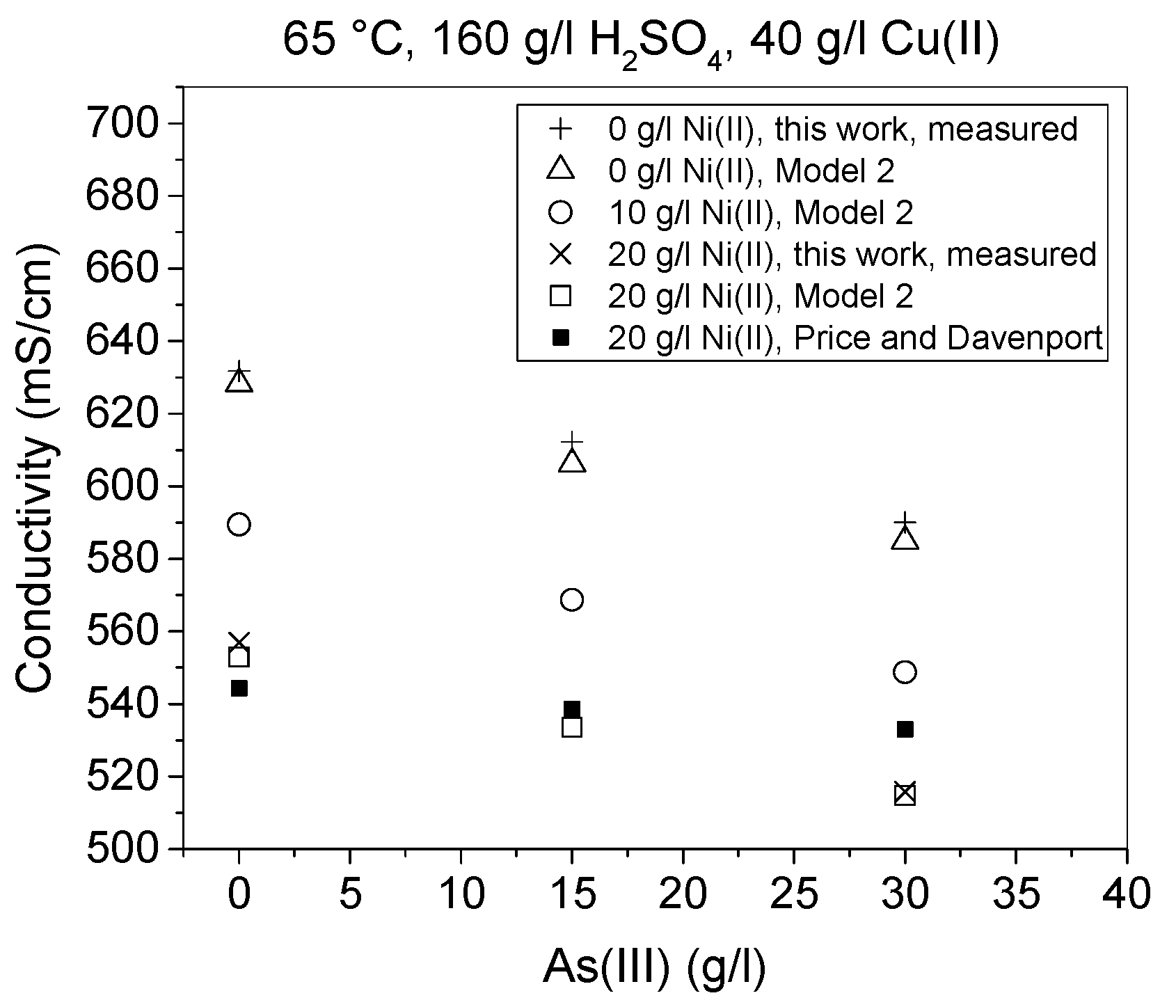
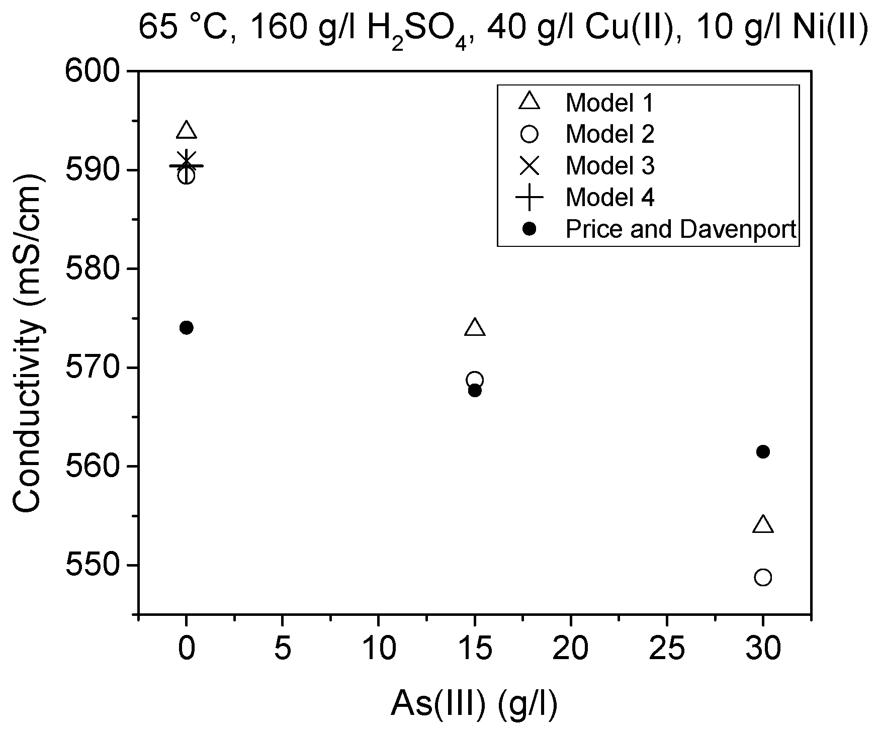
The effects of temperature, Cu(II), As(III) and Ni(II) on conductivity are presented in Figure 9, Figure 10 and Figure 11. In addition to conductivity data calculated by Models 1–4, these figures present the corresponding literature values and in Figure 10 five measured values are also shown. The equation defined by Subbaiah and Das [8] was, however, not used in these comparisons, since it did not reproduce the values they presented in their paper even when their own parameters were used. This is probably due to the fact that their equation did not contain a Cu term, which possibly caused the discrepancy as that error was at minimum at low Cu(II) concentrations.

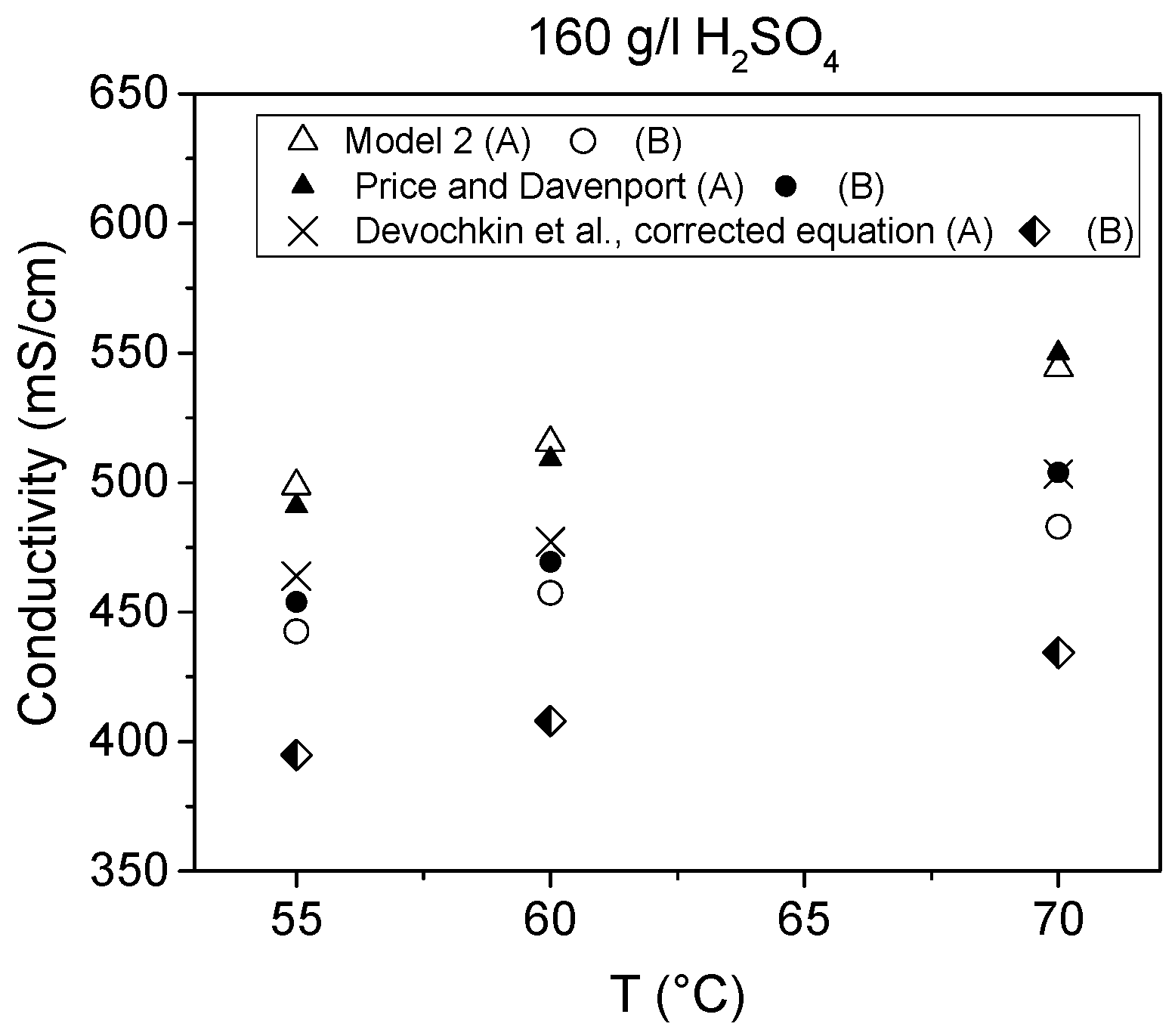
Conductivity results obtained in this work were shown to be in good agreement with the previous research work of Price and Davenport [6]. Nevertheless, arsenic was shown to affect the conductivity slightly more and temperature less than determined by previous works [6,10]. Comparison of the results from this work to the equivalent results of Price and Davenport [6], Kern and Chang [10] and Devochkin et al. [12] shows that there were some differences between them. The conductivity values were seen to be lower in [12] than in the other studies. Conversely, the effect of temperature seemed to be similar according to [12] and this work. These comparisons are presented in Figure 9, where the equation by Devochkin et al. has been corrected due to an error in the sign of the Cu(II) concentration, which was noticed when testing the equation with their parameters and comparing the results to their measured values.

Table 3. Comparison of values defined with Models 1–4 to equivalent values from Price and Davenport [6], Devochkin et al. [12] and to measured values from Kern and Chang [10].

T (°C)	Concentration (g/L)				κ (mS/cm)
					Model				Price and Davenport	Kern and Chang	Devochkin et al.
	H2SO4	Cu(II)	Ni(II)	As(III)	1	2	3	4
55	135	35	0	0	538.4	534.0	536.9	528.3	527.3	530.7	-
55	135	35	30	0	453.4	440.9	472.1	456.1	458.4	444.0	-
55	135	35	0	30	504.8	498.9	-	-	516.7	523.1	-
55	135	35	0	40	493.6	487.7	-	-	513.2	519.4	-
55	150	50	18	0	478.0	475.0	485.8	479.9	477.8	-	446.13

presents a comparison of values calculated with Models 1–4 and the model of Price and Davenport [6], Devochkin et al. [12] and measurements of Kern and Chang [10]. The model of Devochkin et al. was designed to determine conductivity from electrolytes without As(III) and with a constant Cu(II)/Ni(II) ratio; therefore, for that reason, their model was not used with all parameter combinations. The conductivity value determined using their model was lower than the other equivalent values, as can be observed in Figure 7. The values predicted by Models 1–4 were in good agreement with the values measured (Figure 8).

Furthermore, it can be seen that the values defined using the models detailed in this work also show a good correlation with both Kern and Chang’s results [10] and Price and Davenport (who reported a good agreement the results of Kern and Chang) [6]. According to this research, arsenic decreases conductivity and an improved model can be constructed.

4. Conclusions

In this work the conductivity of the copper electrorefining electrolyte was investigated as a function of temperature (50–70 °C) and concentrations of copper (Cu(II), 40–60 g/L), nickel (Ni(II), 0–20 g/L), arsenic (As(III), 0–30 g/L) and sulfuric acid (160–220 g/L). In total, 165 different combinations of these factors were studied.

The measured data showed that conductivity was increased by a decrease in Cu(II), Ni(II) and As(III) concentration and increased with increasing temperature and acidity. As(III) appeared to affect the conductivity in more complicated ways than would be expected based on findings from the literature. In addition, it was observed that the untreated measured data was shown to be slightly skewed.

The results were treated using factorial analysis, and as a result four different electrolyte conductivity models were created. Conductivity was measured reliably, and thus the models from the conductivity results were constructed directly. Combined effects were also detected, but the effects were minor compared to the effects of single factors.

Model 1 was constructed from untreated conductivity data with terms of [H₂SO₄]² and T². Model 2 was constructed from logarithmic values of conductivity, also with additional terms of [H₂SO₄]² and T². Models 3 and 4 were constructed from untreated data by neglecting the measurement series with arsenic, and Model 4 with additional terms of [H₂SO₄]² and T². The four models constructed were all valid and had high correlation coefficients. In addition, the reproducibility was good, and the models did not suffer from a lack of fit. The most accurate models based on the best R², Q² and model validity were Model 2 and Model 4 (Figure 8 and Table 2).

Overall, this work provides improved models for copper electrolyte conductivity both in the presence and absence of arsenic. In particular, As(III) is shown to cause slight non-linearity and decrease conductivity more than previously reported, whereas temperature is shown to affect the electrolyte conductivity slightly less.