
Uncertainty Representation Method for Open Pit Optimization Results Due to Variation in Mineral Prices

Abstract
:1. Introduction
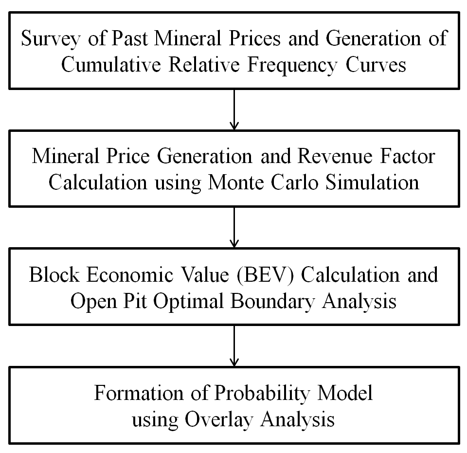
2. Methods
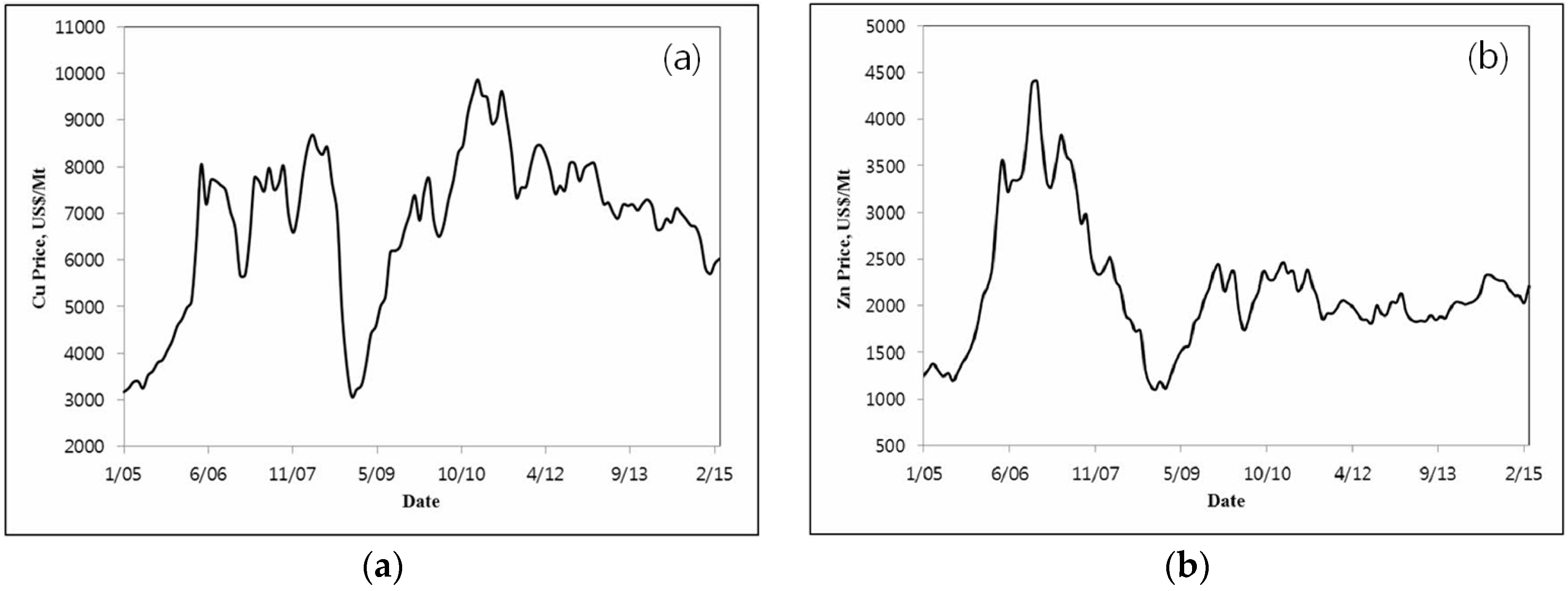
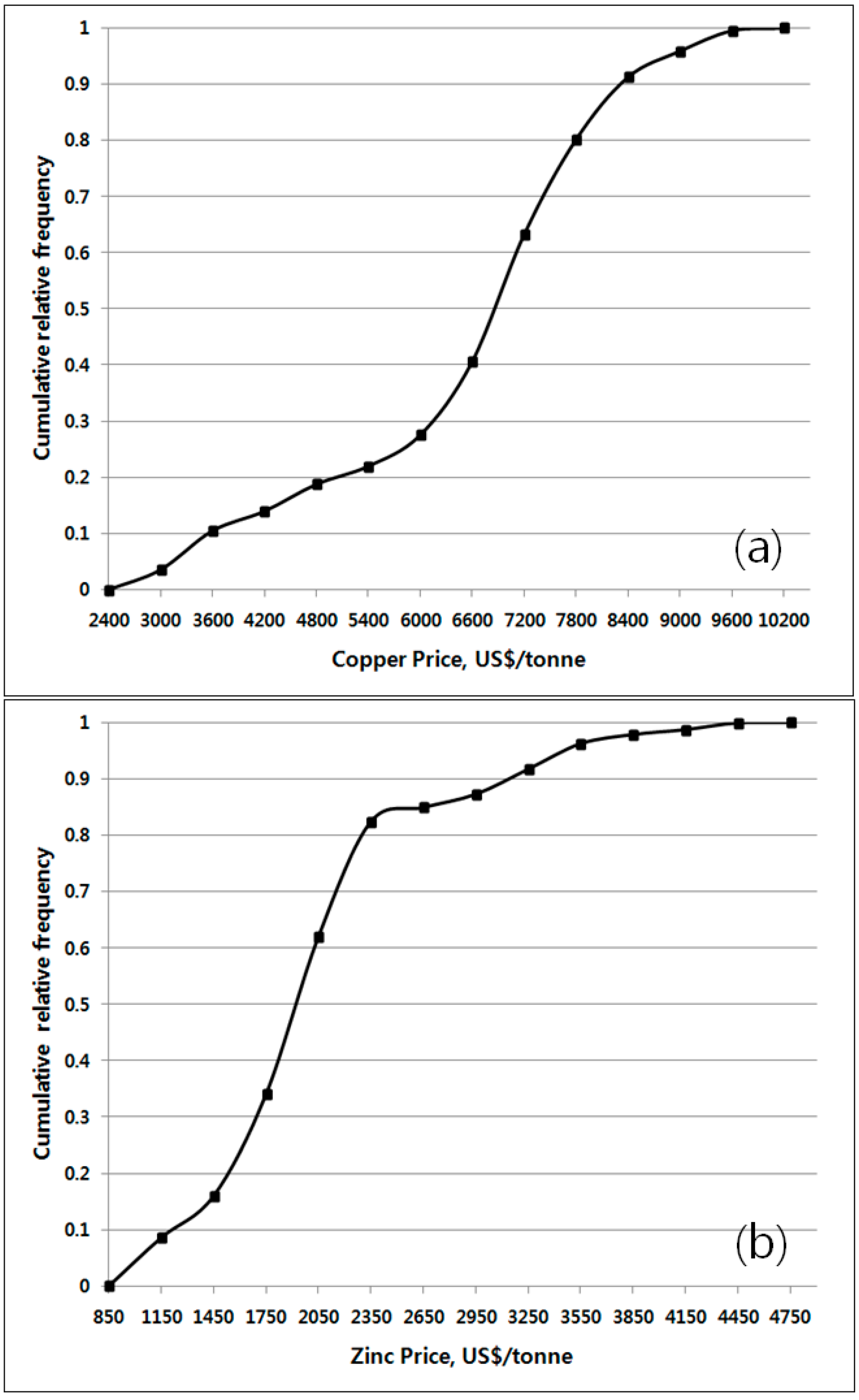
2.1. Survey of Past Mineral Prices and Generation of Cumulative Relative Frequency Curves
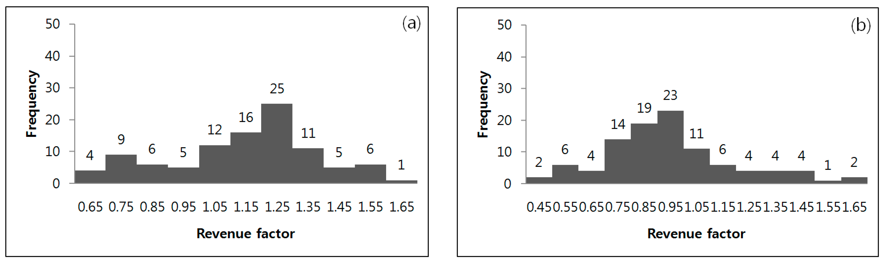
2.2. Mineral Price Generation and Revenue Factor Calculation Using Monte Carlo Simulation
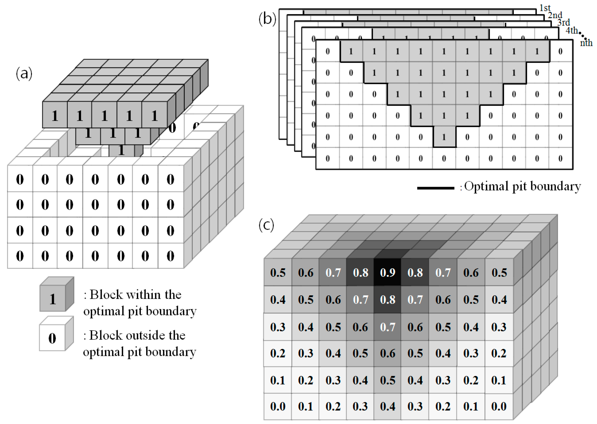
2.3. Block Economic Value (BEV) Calculation and Open Pit Optimal Boundary Analysis
2.4. Formation of Probability Model Using Overlay Analysis
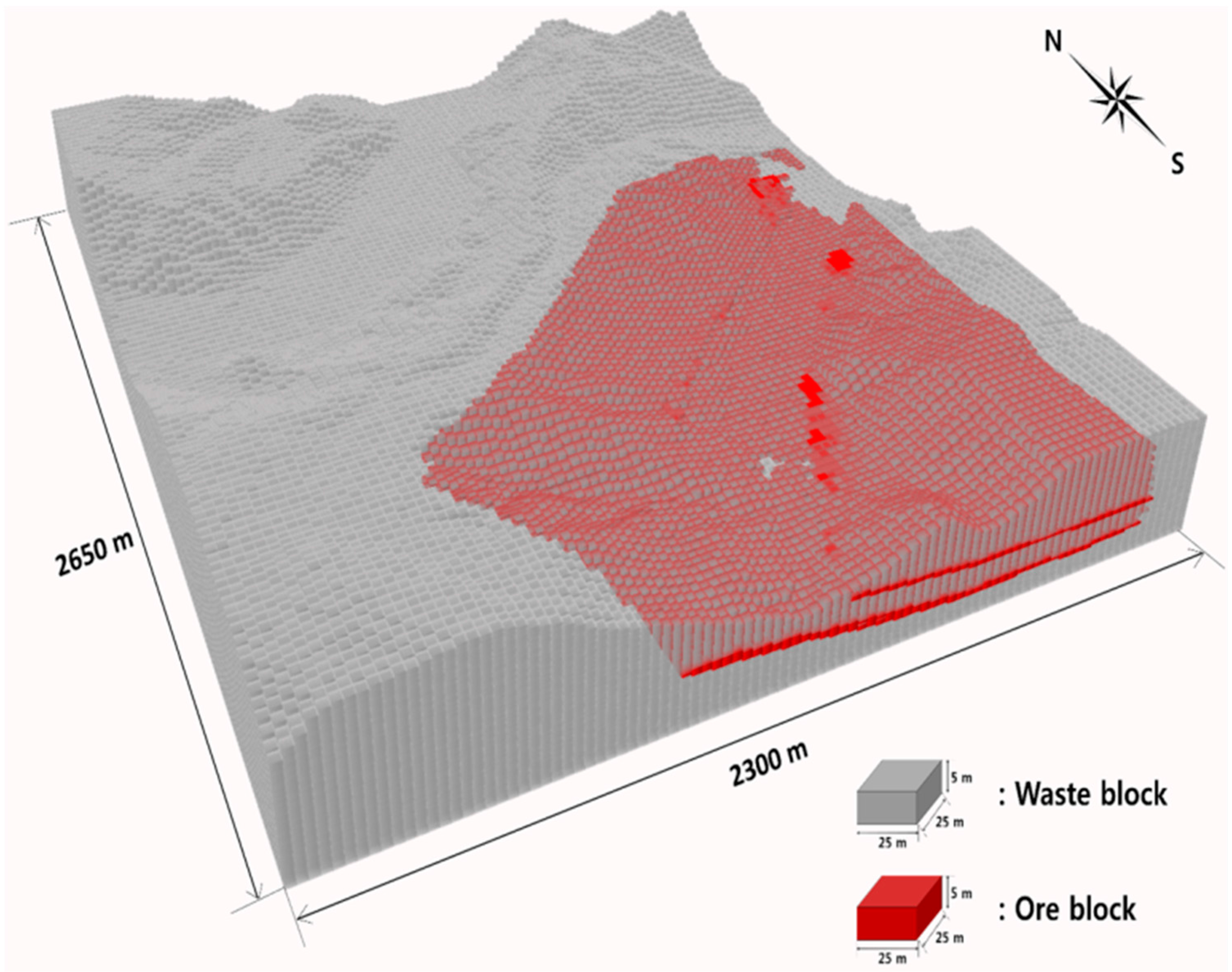
3. Study Area and Data
4. Results
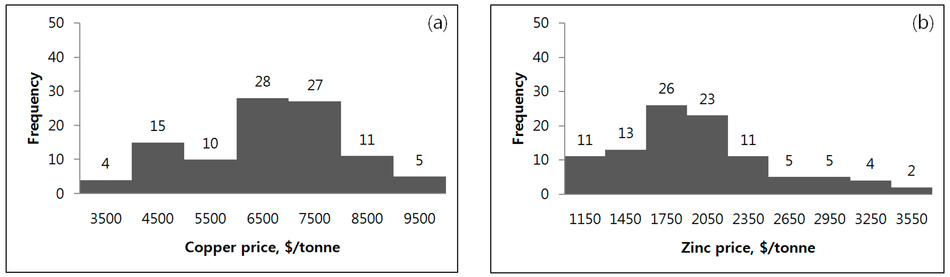
4.1. Results of Cumulative Relative Frequency Curves of Copper and Zinc
4.2. Revenue Factor of Copper and Zinc Price Calculation Results Using Monte Carlo Simulation
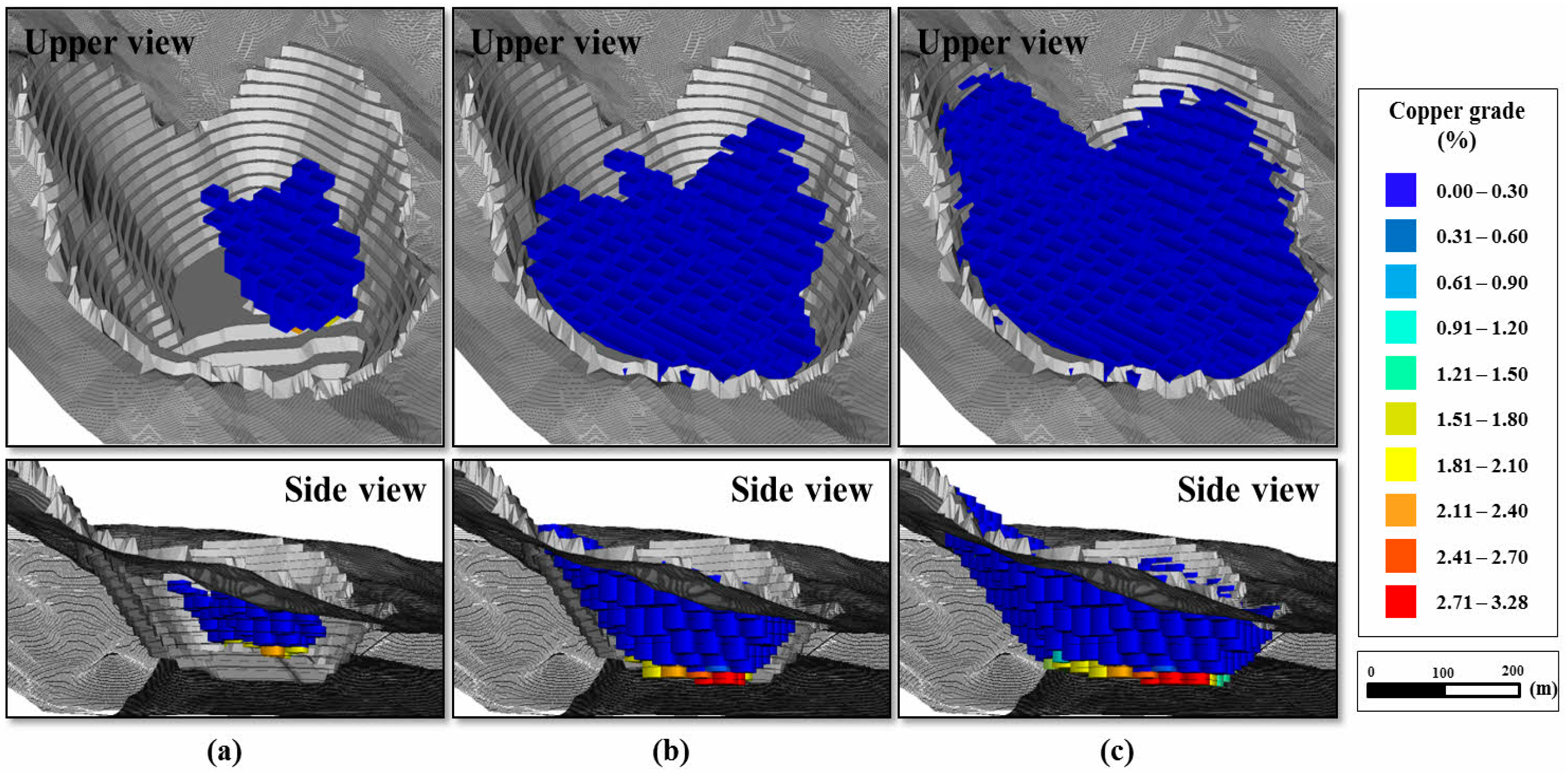
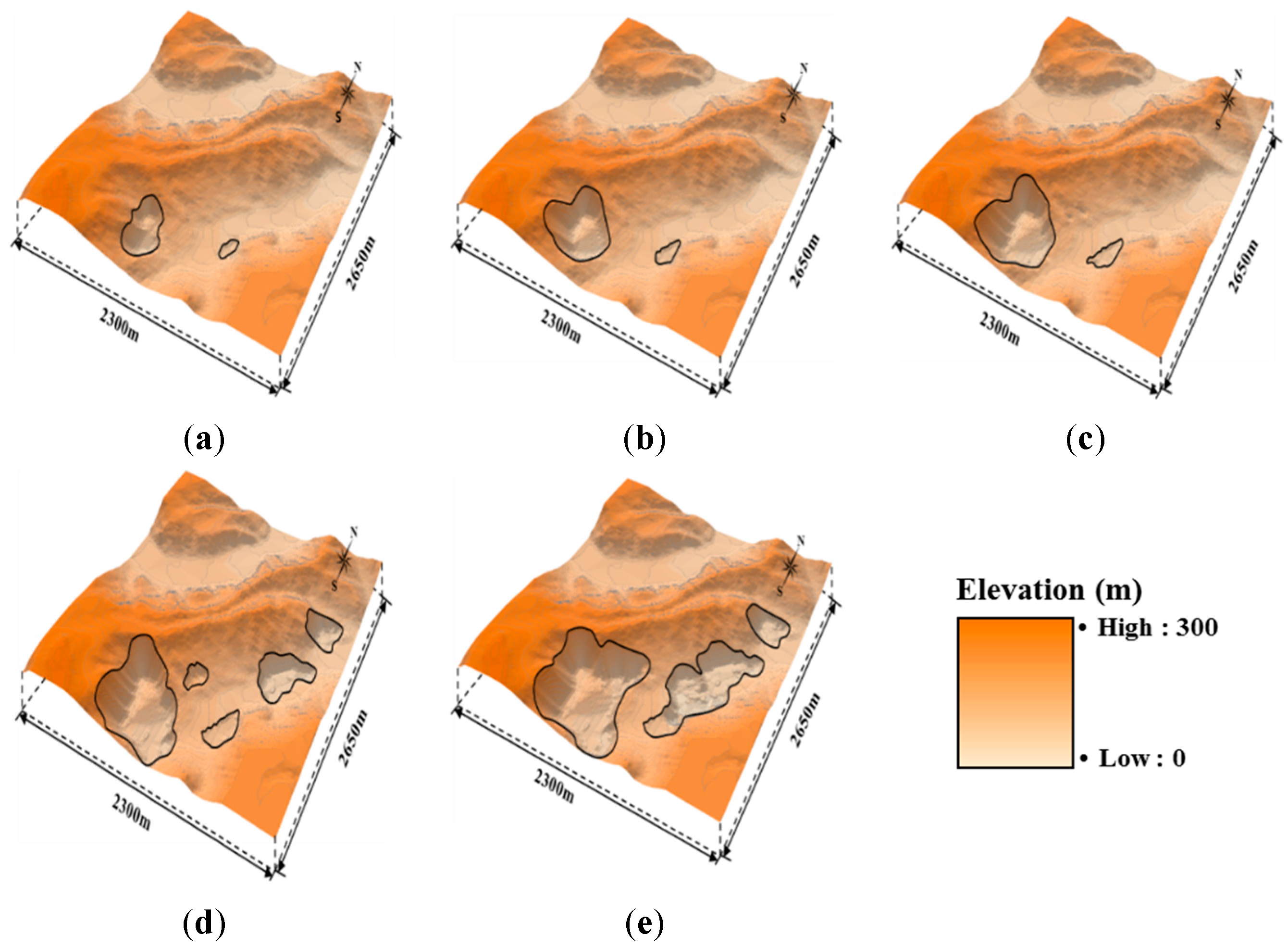
4.3. BEV Calculation and Open Pit Optimal Boundary Analysis Results
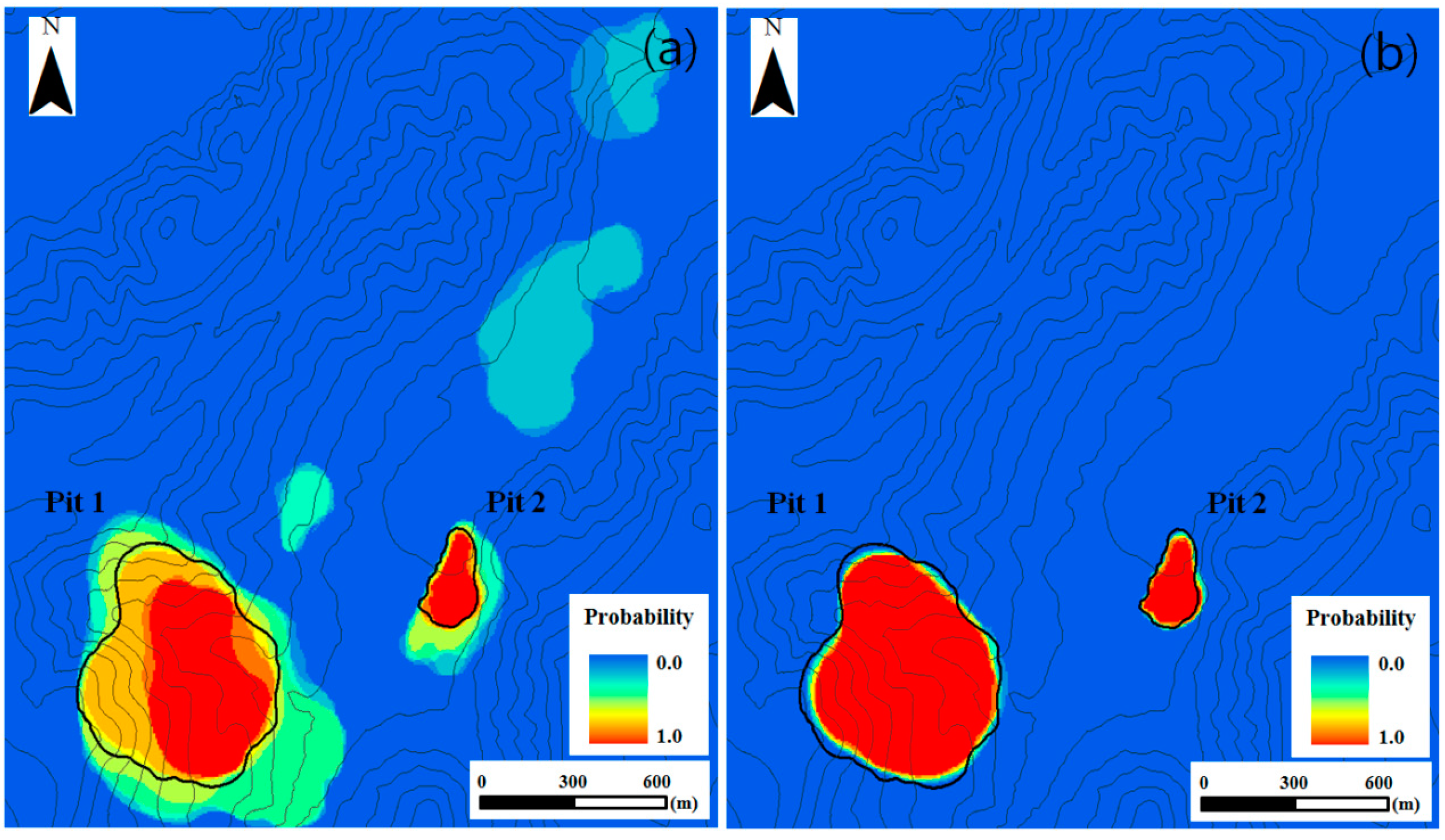
4.4. Results of Probability Model Formation
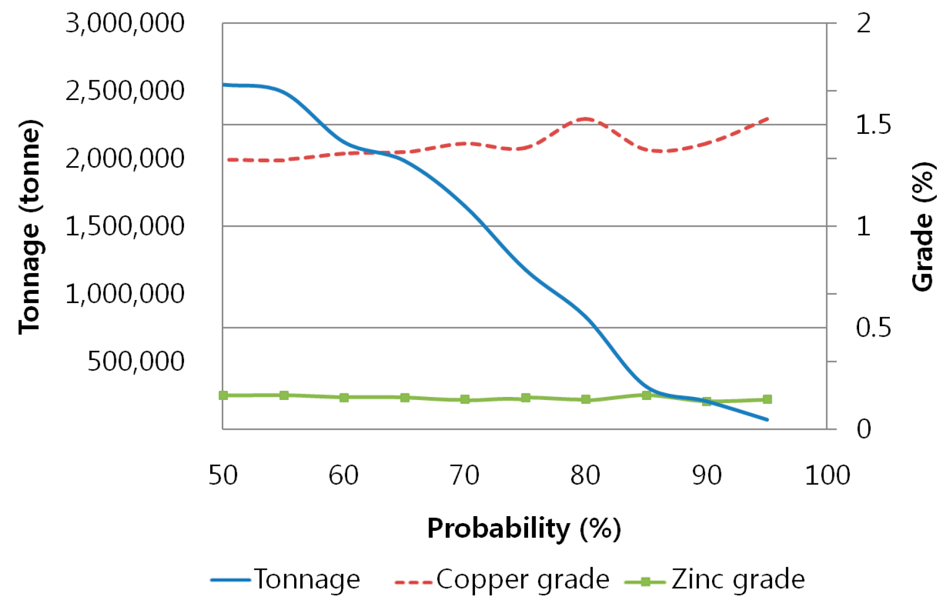
4.5. Deposit Reserve Estimation as a Function of Confidence Level
5. Discussion
6. Conclusions
Acknowledgments
Author Contributions
Conflicts of Interest
References
- Lerchs, H.; Grossmann, L. Optimum design of open-pit mines. Can. Min. Metall. Bull. 1965, 58, 47–54. [Google Scholar]
- Picard, J.C. Maximal closure of a graph and applications to combinatorial problems. J. Manag. Sci. 1976, 22, 1268–1272. [Google Scholar] [CrossRef]
- David, M.; Dowd, P.A.; Korobov, S. Forecasting departure from planning in open pit design and grade control. In Proceedings of the 12th International APCOM Symposium, Golden, CO, USA, 8–12 April 1974.
- Lane, K.F. The Economic Definition of Ore: Cutoff Grade in Theory and Practice, 1st ed.; Mining Journal Books Limited: London, UK, 1988; pp. 1–147. [Google Scholar]
- Caccetta, L.; Giannini, L.M. An application of discrete mathematics in the design of an open pit mine. Discrete Appl. Math. 1988, 21, 1–19. [Google Scholar] [CrossRef]
- Berlanga, J.M.; Cardona, R.; Ibarra, M.A. Recursive formulae for the floating cone algorithm. Int. J. Surf. Min. Reclam. Environ. 1989, 3, 141–150. [Google Scholar] [CrossRef]
- Zhao, Y.; Kim, Y.C. A new ultimate pit limit design algorithm. In Proceedings of the International 23rd APCOM Symposium, Tucson, AZ, USA, 7–11 April 1992.
- Dowd, P.A.; Onur, A.H. Open-pit optimization—Part 1: Optimal open pit design. Trans. Inst. Min. Metall. 1993, 102, A95–A104. [Google Scholar]
- Yamatomi, J.; Mogi, G.; Akaike, A.; Yamaguchi, U. Selective extraction dynamic cone algorithm for three-dimensional open pit designs. In Proceedings of the 25th International APCOM Symposium, Brisbane, Australia, 9–14 July 1995.
- Underwood, R.; Tolwinski, B. A mathematical programming viewpoint for solving the ultimate pit problem. Eur. J. Oper. Res. 1998, 107, 96–107. [Google Scholar] [CrossRef]
- Hochbaum, D.S.; Chen, A. Performance analysis and best implementations of old and new algorithms for the open-pit mining problem. Oper. Res. 2000, 48, 894–914. [Google Scholar] [CrossRef]
- Gershon, M.E. Mine scheduling optimization with mixed integer programming. Min. Eng. 1983, 35, 351–354. [Google Scholar]
- Busnach, E.; Mehrez, A.; Sinuany-Stern, Z. A production problem in phosphate mining. J. Oper. Res. Soc. 1985, 36, 285–288. [Google Scholar] [CrossRef]
- Gershon, M. Heuristic approaches for mine planning and production scheduling. Int. J. Min. Geol. Eng. 1987, 5, 1–13. [Google Scholar] [CrossRef]
- Souza, M.J.F.; Coelho, I.M.; Ribas, S.; Santos, H.G.; Merschmann, L.H.C. A hybrid heuristic algorithm for the open-pit mining operational planning problem. Eur. J. Oper. Res. 2010, 207, 1041–1051. [Google Scholar] [CrossRef]
- Cullenbine, C.; Wood, R.K.; Newman, A. A sliding time window heuristic for open pit mine blcok sequencing. Optim. Lett. 2011, 5, 365–377. [Google Scholar] [CrossRef]
- Chicoisne, R.; Espinoza, D.; Goycoolea, M.; Moreno, E.; Rubio, E. A new algorithm for the open-pit mine scheduling problem. Oper. Res. 2012, 60, 517–528. [Google Scholar] [CrossRef]
- Epstein, R.; Goic, M.; Weintraub, A.; Catalán, J.; Santibáñez, P.; Cancino, R.; Gaete, S.; Aguayo, A.; Caro, F. Optimizing long-term production plans in underground and open-pit copper mines. Oper. Res. 2012, 60, 4–17. [Google Scholar] [CrossRef]
- Dendy, B.; Schofield, D. Open-pit design and scheduling by use of genetic algorithms. Trans. Inst. Min. Metall. 1994, 103, A21–A26. [Google Scholar]
- Dendy, B.; Schofield, D. The use of genetic algorithms in underground mine scheduling. In Proceedings of the 25th International APCOM Symposium, Brisbane, Australia, 9–14 July 1995.
- Elevli, B. Open pit mine design and extraction sequencing by use of OR and AI concepts. Int. J. Surf. Min. Reclam. Environ. 1995, 9, 149–153. [Google Scholar] [CrossRef]
- Tolwinski, B.; Underwood, R. A scheduling algorithm for open pit mines. IMA J. Manag. Math. 1996, 7, 247–270. [Google Scholar] [CrossRef]
- Caccetta, L.; Hill, S.P. An application of branch and cut to open pit mine scheduling. J. Glob. Optim. 2003, 27, 349–365. [Google Scholar] [CrossRef]
- Boland, N.; Dumitrescu, I.; Foyland, G.; Gleixner, M. LP-based disaggregation approaches to solving the open pit mining production scheduling problem with block processing selectivity. Comput. Oper. Res. 2009, 36, 1064–1089. [Google Scholar] [CrossRef]
- Bienstock, D.; Zuckerberg, M. Solving LP relaxations of large-scale precedence constrained problems. In Proceedings of the 14th international conference on IPCO (Integer Programming and Cominatorial Optimisation), Lausanne, Switzerland, 9–11 June 2010.
- Kumral, M.; Dowd, P.A. A simulated annealing approach to mine production scheduling. J. Oper. Res. Soc. 2005, 56, 922–930. [Google Scholar] [CrossRef]
- Ramazan, S. The new fundamental tree algorithm for production scheduling of open pit mines. Eur. J. Oper. Res. 2007, 177, 1153–1166. [Google Scholar] [CrossRef]
- Bley, A.; Boland, N.; Fricke, C.; Froyland, G. A strengthened formulation and cutting planes for the open pit mine production scheduling problem. Comput. Oper. Res. 2010, 37, 1641–1647. [Google Scholar] [CrossRef]
- Liu, S.Q.; Kozan, E. New graph-based algorithms to efficiently solve large scale open pit mining optimisation problems. Expert Syst. Appl. 2016, 43, 59–65. [Google Scholar] [CrossRef]
- Godoy, M. The Effective Management of Geological Risk in Long-Term Production Scheduling of Open Pit Mines. Ph.D. Thesis, University of Queensland, St Lucia, Australia, 2003. [Google Scholar]
- Menabde, M.; Foyland, G.; Stone, P.; Yeates, G. Mining schedule optimisation for conditionally simulated orebodies. In Proceedings of the International Symposium on Orebody Modelling and Stategic Mine Planning: Uncertainty and Risk Management, Perth, WA, USA, 22–24 November 2004.
- Costa Lima, G.A.; Suslick, S.B. Estimating the volatility of mining projects considering price and operating cost uncertainties. J. Resour. Policy 2006, 31, 86–94. [Google Scholar] [CrossRef]
- Golamnejad, J.; Osanloo, M.; Karimi, B. A chance-constrained programming approach for open pit long-term production scheduling in stochastic environments. J. S. Afr. Inst. Min. Metall. 2006, 106, 105–114. [Google Scholar]
- Dimitrakopoulos, R.; Abdel Sabour, S.A. Evaluating mine plans under uncertainty: Can the real options make a difference? J. Resour. Policy 2007, 32, 116–125. [Google Scholar] [CrossRef]
- Ramazan, S.; Dimitrakopoulos, R. Stochastic optimization of long term production scheduling for open pit mines with a new integer programming formulation. In Proceedings of the Orebody Modelling and Strategic Mining Planning Symposium, Perth, Australia, 22–24 November 2004.
- Boland, N.; Dumitrescu, I.; Froyland, G. A Multistage Stochastic Programming Approach to Open Pit Mine Production Scheduling with Uncertain Geology. Available online: http://www.optimization-online.org/DB_HTML/2008/10/2123.html (accessed on 22 February 2016).
- Akbari, A.D.; Osanloo, M.; Shirazi, M.A. Determination of ultimate pit limits in open mines using real option approach. IUST Int. J. Eng. Sci. 2008, 19, 23–38. [Google Scholar]
- Albor, F.; Dimitrakopoulos, R. Algorithmic approach to pushback design based on stochastic programming: Method, application and comparisons. Trans. Inst. Min. Metall. 2010, 119, 88–101. [Google Scholar]
- Abdel Sabour, S.A.; Dimitrakopoulos, R. Incorporating geological and market uncertainties and operational flexibility into open pit mine design. J. Min. Sci. 2011, 47, 191–201. [Google Scholar] [CrossRef]
- Evatt, G.W.; Soltan, M.O.; Johnson, P.V. Mineral reserves under price uncertainty. Resour. Policy 2012, 37, 340–345. [Google Scholar] [CrossRef]
- Lamghari, A.; Dimitrakopoulos, R. A diversified Tabu search approach for the open-pit mine production scheduling problem with metal uncertainty. Eur. J. Oper. Res. 2012, 222, 642–652. [Google Scholar] [CrossRef]
- Asad, M.W.A.; Dimitrakopoulos, R. Implementing a parametric maximum flow algorithm for optimal open pit mine design under uncertain supply and demand. J. Oper. Res. Soc. 2013, 64, 185–197. [Google Scholar] [CrossRef]
- Alonso-Ayuso, A.; Carvallo, F.; Escuderto, L.F.; Guignard, M.; Pi, J.; Puranmalka, R.; Weintraub, A. Medium range optimization of copper extraction planning under uncertainty in future copper prices. Eur. J. Oper. Res. 2014, 233, 711–726. [Google Scholar] [CrossRef]
- Kizilkale, A.C.; Dimitrakopoulos, R. Optimizing mining rates under financial uncertainty in global mining complexes. Int. J. Prod. Econ. 2014, 158, 359–365. [Google Scholar] [CrossRef]
- Hall, G. Multi-mine better than multiple mines. In Proceedings of the Orebody Modelling and Strategic Mining Planning Symposium, Perth, Australia, 22–24 November 2004.
- Elahizeyni, E.; Kakaie, R.; Yousefi, A. A new algorithm for optimum open pit design: Floating cone method III. J. Min. Environ. 2011, 2, 118–125. [Google Scholar]
- Magassouba, M. OK Block Model Versus MIK Block Model: Optimization of the Profit Cut-off at the Northern Nevada Pit, USA. Master’s Thesis, University of Nevada, Reno, NV, USA, August 2006. [Google Scholar]
- Hustralid, W.; Kuchta, M.; Martin, R. Open Pit Mine Planning and Design Volume 1—Fundamentals, 3rd ed.; CRC Press: Leiden, The Netherlands, 2013; pp. 409–501. [Google Scholar]


| Class Interval ($/tonne) | Frequency | Relative Frequency | Cumulative Relative Frequency |
|---|---|---|---|
| 2700–3300 | 92 | 0.0353 | 0.0353 |
| 3300–3900 | 181 | 0.0694 | 0.1047 |
| 3900–4500 | 91 | 0.0349 | 0.1396 |
| 4500–5100 | 125 | 0.0479 | 0.1876 |
| 5100–5700 | 84 | 0.0322 | 0.2198 |
| 5700–6300 | 144 | 0.0552 | 0.2750 |
| 6300–6900 | 340 | 0.1304 | 0.4054 |
| 6900–7500 | 590 | 0.2263 | 0.6318 |
| 7500–8100 | 442 | 0.1695 | 0.8013 |
| 8100–8700 | 290 | 0.1112 | 0.9125 |
| 8700–9300 | 121 | 0.0464 | 0.9590 |
| 9300–9900 | 95 | 0.0364 | 0.9954 |
| 9900–10,500 | 12 | 0.0046 | 1.0000 |
| Class Interval ($/tonne) | Frequency | Relative Frequency | Cumulative Relative Frequency |
|---|---|---|---|
| 1000–1300 | 224 | 0.0859 | 0.0859 |
| 1300–1600 | 193 | 0.0740 | 0.1600 |
| 1600–1900 | 470 | 0.1803 | 0.3402 |
| 1900–2200 | 729 | 0.2796 | 0.6199 |
| 2200–2500 | 532 | 0.2041 | 0.8239 |
| 2500–2800 | 66 | 0.0253 | 0.8493 |
| 2800–3100 | 61 | 0.0234 | 0.8727 |
| 3100–3400 | 116 | 0.0445 | 0.9171 |
| 3400–3700 | 118 | 0.0453 | 0.9624 |
| 3700–4000 | 42 | 0.0161 | 0.9785 |
| 4000–4300 | 23 | 0.0088 | 0.9873 |
| 4300–4600 | 31 | 0.0119 | 0.9992 |
| 4600–4900 | 2 | 0.0008 | 1.0000 |
| Input Parameters | Unit | Copper | Zinc |
|---|---|---|---|
| Price of metal (P) | $/tonne | 6027.96 | 2206.90 |
| Recovery (r) | % | 0.90 | 0.65 |
| Selling cost (SC) | $/tonne | 120.00 | 120.00 |
| Mining cost (MC) | $/tonne | 2.70 | 2.70 |
| Processing cost (PC) | $/tonne | 40.08 | 40.08 |
© 2016 by the authors; licensee MDPI, Basel, Switzerland. This article is an open access article distributed under the terms and conditions of the Creative Commons by Attribution (CC-BY) license (http://creativecommons.org/licenses/by/4.0/).
Share and Cite
Baek, J.; Choi, Y.; Park, H.-s. Uncertainty Representation Method for Open Pit Optimization Results Due to Variation in Mineral Prices. Minerals 2016, 6, 17. https://doi.org/10.3390/min6010017
Baek J, Choi Y, Park H-s. Uncertainty Representation Method for Open Pit Optimization Results Due to Variation in Mineral Prices. Minerals. 2016; 6(1):17. https://doi.org/10.3390/min6010017
Chicago/Turabian StyleBaek, Jieun, Yosoon Choi, and Han-su Park. 2016. "Uncertainty Representation Method for Open Pit Optimization Results Due to Variation in Mineral Prices" Minerals 6, no. 1: 17. https://doi.org/10.3390/min6010017