Flotation Bubble Delineation Based on Harris Corner Detection and Local Gray Value Minima

Abstract

Froth image segmentation is an important and basic part in an online froth monitoring system in mineral processing. The fast and accurate bubble delineation in a froth image is significant for the subsequent froth surface characterization. This paper proposes a froth image segmentation method combining image classification and image segmentation. In the method, an improved Harris corner detection algorithm is applied to classify froth images first. Then, for each class, the images are segmented by automatically choosing the corresponding parameters for identifying bubble edge points through extracting the local gray value minima. Finally, on the basis of the edge points, the bubbles are delineated by using a number of post-processing functions. Compared with the widely used Watershed algorithm and others for a number of lead zinc froth images in a flotation plant, the new method (algorithm) can alleviate the over-segmentation problem effectively. The experimental results show that the new method can produce good bubble delineation results automatically. In addition, its processing speed can also meet the online measurement requirements.

1. Introduction

Froth flotation is a selective separation process that is widely used in mineral processing to extract valuable minerals. Froth is a three-phase structure comprising air bubbles, solids and water [1]. The modeling and the control of flotation processes are challenging because of the inherently chaotic nature of the underlying microscopic phenomena. The lack of sufficiently accurate and reliable process measurements intensifies the difficulty. In fact, the control of flotation process depends heavily on various experiences of human operators by looking at the appearance of the froth [2]. The performance thus depends on the operator’s experience and is limited by the absence of physical, quantitative methods for measurement and characterization of the froth [3]. Therefore, methods based on machine vision and image processing have been developed for observation and analysis of froth images, including the application for extraction of bubble size, shape and other physical features [4,5,6]. Moreover, the correlation between these features and the flotation performance also has been studied [7,8].

This paper aims to extract the bubble size and shape based on image segmentation techniques. Here it should be noted that the bubbles (in this paper) are the bubbles on a froth surface. Although there exists remarkable difference between the surface bubble size distribution and the underlying bubble size distribution [9], Wang and Neethling have found that an empirical formula for the relationship between the above two kinds of bubbles can be used to obtain the underlying bubble size distribution from the surface bubble size distribution effectively [10].

Hence, machine vision based on bubble film size measurement becomes a reasonable solution to interpret the surface bubble structure automatically [5]. The surface bubble size and shape are two of the dominant visual features closely relating to the reagent addition [6,11]. And the surface bubble size can also be used as an effective measurement of bubble stability for the reason that it reflects the extent of bubble coalescence [12]. Zanin et al. used the bubble size on the froth top as one of indicators for froth stability [13]. Furthermore, many researchers have reported the relationship between the bubble size, water recovery, and froth recovery, etc. [9,14]. Hence, by using image processing and analysis, the bubble size estimation in flotation has received a considerable research attention over the years. However, the performance of the existing froth image segmentation methods is not satisfactory due to the uneven illumination and different noise. A froth image usually contains thousands of color mineral liquid bubbles of different sizes and shapes, with weak intensity boundaries. A bubble is mainly spherical or polyhedral in shape; therefore, the light makes the top part of a bubble with high brightness and the boundary region with low brightness. All the characteristics of a froth image make bubble delineation hard. The traditional edge detection methods often only detect the edges of particles, light reflection areas and black holes. How to achieve an efficient froth image segmentation method has become a major task in this research field.

Wang et al. and Citir et al. proposed their image segmentation algorithms through the usage of bubble edges and sizes [15,16], and their algorithms have succeeded in extracting the bubbles edges. An improved particle swarm optimization algorithm was applied to achieve a more suitable threshold in a froth edge extraction method [17]. A set of Watershed algorithms combined with clustering pre-segmentation and high-low scale distance reconstruction were used to segment color froth images [18], which can conquer the over-segmentation and under-segmentation problems in some cases. However, each of the above algorithms is only suitable for a special case, or it may need human intervention that cannot be automatically applied in the industrial flotation scale online. Some methods based on texture spectrum were also used to estimate bubble sizes [3]. Two recent literature reviews have been carried out by Aldrich et al. and Shean and Cilliers, respectively [19,20]; the previous froth image segmentation methods can be classified into two categories. One is based on mathematical morphology, in which, the Watershed algorithm is the representative one [21]. The Watershed algorithm is a morphological method based on a simulation of the water rising from a set of markers, which is well known as an excellent image segmentation method for the images of the complex and densely packed objects. A Watershed method can obtain a good image segmentation result when the processed image is of more uniform bubble size and shape distributions, but for the images with the large variations of the object sizes and shapes, it is easy to encounter the over-segmentation or under-segmentation problems [22]. In addition, the Watershed algorithm has the disadvantage in computational complexity (a huge number of repeating operations). The other is based on edge detection. The advantages of the method based on edge detection are (1) of a high processing speed; and (2) not affected by the variations of bubble size and shape, but such an algorithm is sensitive to the bubble surface noise in an image of large bubbles. Wang et al. proposed an improved valley edge detection algorithm based on multi-scale analysis [23]. Although the improved algorithm can produce good results for most froth images, the under-segmentation and over-segmentation problems still exist in some cases.

Currently, there are several commercial froth image processing systems, such as FrothMaster (Outokumpu, Espoo, Finland), SmartFroth (UCT, Cape Town, South Africa) and VisioFroth (Metso, Helsinki, Finland). For the bubble size and shape measurement, each of the systems uses its own method according to its flotation image properties, for instance, average size estimation by using statistical analysis for unclear bubble images (e.g., Iron flotation), and the bubble size delineation and measurement by applying the Watershed algorithm combining color information for the images where the bubbles are showing up clearly (e.g., Copper flotation), etc. There is no standard image segmentation algorithm for all the cases. The implementation of a long-term fully automated flotation control system is difficult due to the image segmentation problem.

As requirements from Jin Dong lead zinc flotation plant in China, we designed and developed a new system for flotation monitoring. The key task in the system is image segmentation-bubble delineation. In the testing, the results produced by most existing froth image segmentation algorithms are not satisfactory and their processing speeds are also far from the requirement of an online flotation control system, therefore, a new bubble delineation method is proposed in this study, which is the combination of image classification and image segmentation. The studied method is tested for a large number of lead froth images. The test results show that the new method can produce good image segmentation results than others, and our algorithm has the advantages in low computational complexity and it can effectively reduce the over-segmentation and under-segmentation problems.

2. Froth Image Segmentation on Improved Local Gray Value Minima

2.1. Characteristics of Froth Images

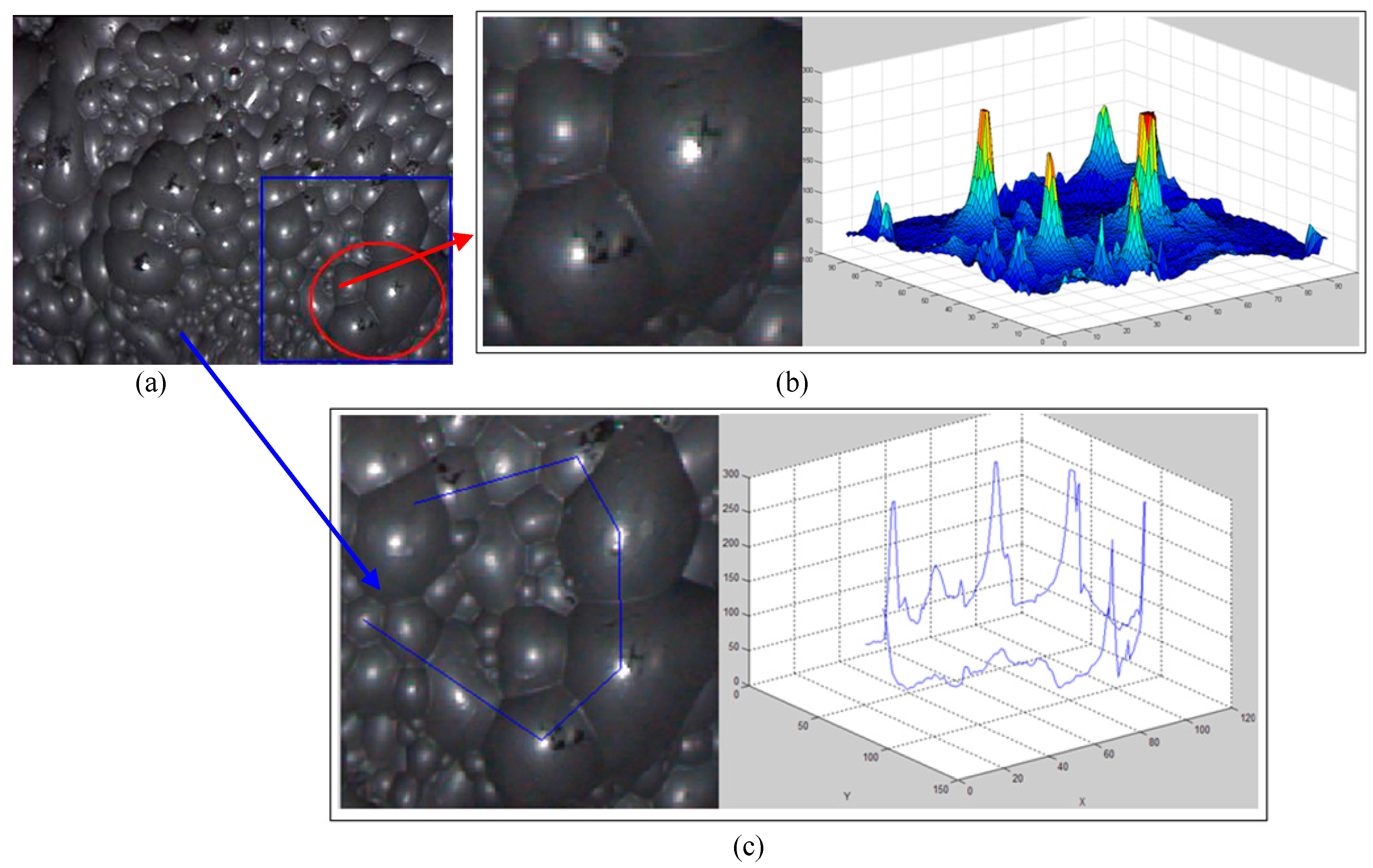
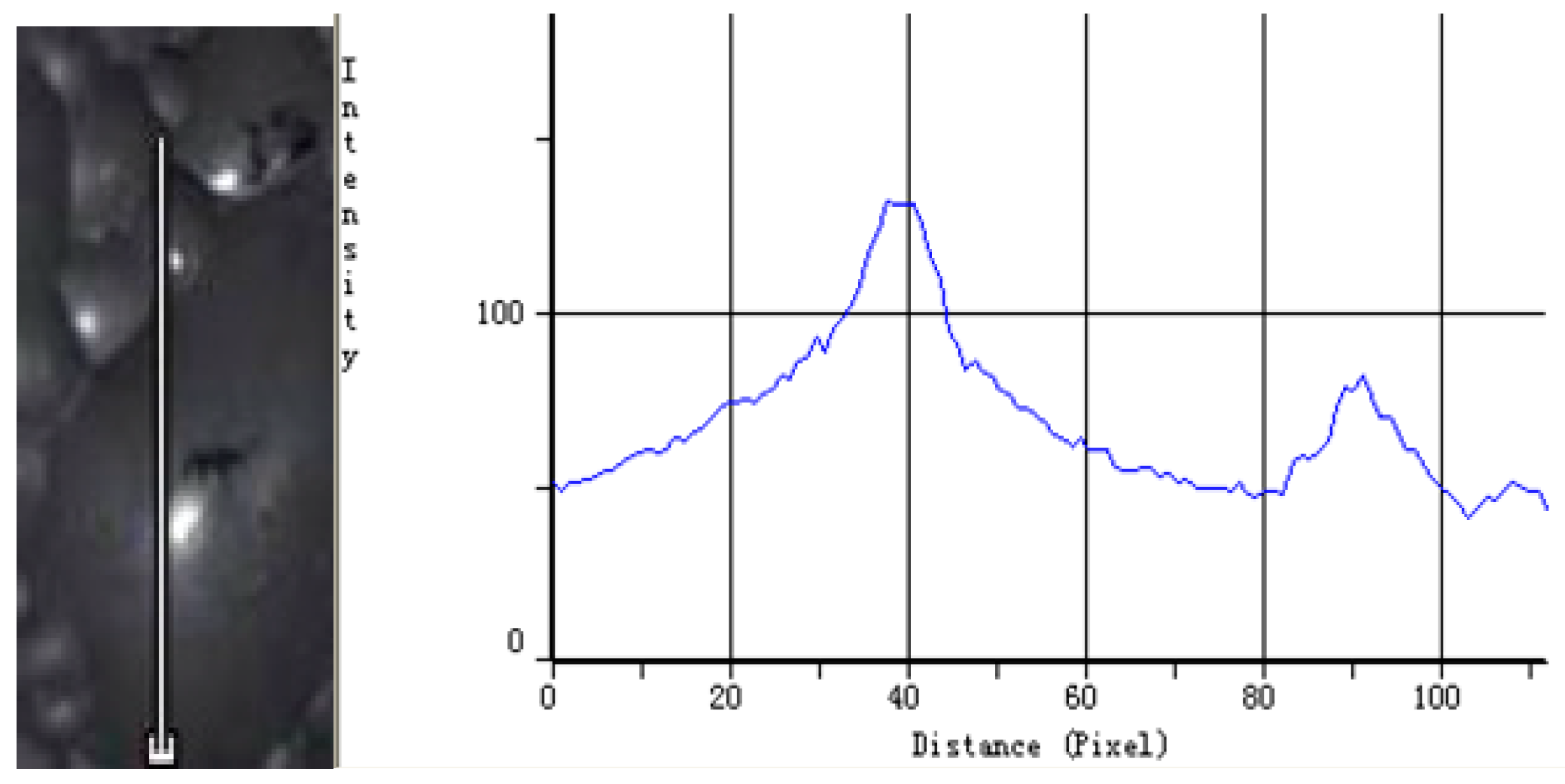
As shown in Figure 1 and Figure 2, due to bubble’s 3D geometry and the light reflection, there exist one or more high gray value regions in each bubble, called “white spot areas”. The boundary regions among the adjacent bubbles have low gray values, called “boundary areas”, where the local gray value minima points can be considered as bubble boundary pixels. 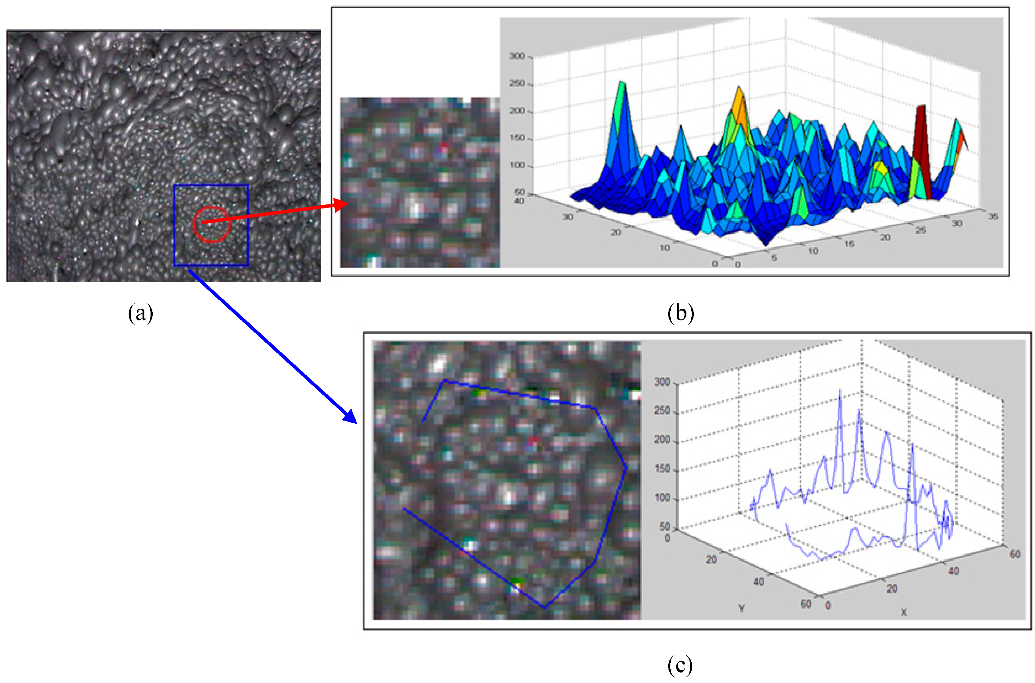For images of large bubbles, the number of bubbles in an image is small, and the white spot areas are large regions and the boundary regions are long on average (see Figure 1); for images of small and fine bubbles, the number of bubbles in an image is great, and the white spot areas are small regions and the boundary regions are short narrow on average (see Figure 2). It is noted that all of the images used in this paper are the lead froth images obtained from Jin Dong flotation plant in China. In the plant, the raw ore mainly contains lead and zinc, and also includes sulfur, iron, silver, copper and other sulfide minerals, and the Gangue minerals include quartz, feldspar, pyroxene, garnet, chlorite and other silicate minerals. Hence, for the image segmentation, the flotation images are complicated; we have to study a new image segmentation algorithm.

For the above reasons, before image segmentation, a froth image can be classified into the class of large or non-large bubbles. For an image of large bubbles, a large template is used in the subsequent local gray value minima detection process; the small template is used for an image of non-large bubbles.

Figure 1. Gray value characteristics of the image of large bubbles. (a) a large bubble image; (b) left: a part of the image (a); right: the 3D surface of the left image; (c) left: large bubbles and the profile line; right: the gray level histogram of the profile corresponding to the left image.

Figure 1. Gray value characteristics of the image of large bubbles. (a) a large bubble image; (b) left: a part of the image (a); right: the 3D surface of the left image; (c) left: large bubbles and the profile line; right: the gray level histogram of the profile corresponding to the left image.

2.2. Edge Detection on Improved Local Gray Value Minima

According to the above analyses of the gray value variations in a froth image, it can be concluded that if all the local gray value minima points are detected, the information of the minima points can be used for bubble delineation on edges.

For a large bubble, its boundary region is a long border area, and there are often multiple local valley points in its boundary area. Moreover, because of the rough surface of a large bubble, the gray value distribution on the bubble surface is quite uneven, as shown in Figure 3, in other words, a number of the local gray value minima points exist in the area, and these points belong to the non-bubble boundary points. For this kind of information, once directly extracted, this non-boundary information often form many closed curves that are very difficult to be removed by subsequent non-boundary information filters. Thus, to make the non-bubble boundary information as less as possible, for large bubbles, the segmentation algorithm adopts a large sized kernel for the local gray value minima point detection, e.g., 5 × 5 or 7 × 7, therefore, the comparison distance is increased. To further remove the speckle noise on a froth surface, the algorithm uses the gradation weighted average gray values in a local area for comparison instead of a single pixel gray value.

Figure 2. Gray value characteristic of the image of small bubbles. (a) A small bubble image; (b) left: a part of the image (a); right: the 3D surface of the left image; (c) left: small bubbles and the profile line; right: the gray level histogram of the profile corresponding to the left image.

Figure 2. Gray value characteristic of the image of small bubbles. (a) A small bubble image; (b) left: a part of the image (a); right: the 3D surface of the left image; (c) left: small bubbles and the profile line; right: the gray level histogram of the profile corresponding to the left image.

Figure 3. Gray value variation between two bubbles. Left: large bubble and the profile line; Right: the gray value histogram of the profile corresponding to the left image from bottom to top.

Figure 3. Gray value variation between two bubbles. Left: large bubble and the profile line; Right: the gray value histogram of the profile corresponding to the left image from bottom to top.

Based on the above idea, an edge detection method based on the improved local gray value minima is designed and developed to extract bubble edges.

We use $f(i,j)$ to denote an original froth image, $g(i,j)$ is for its edge image, and all the values in $g(i,j)$ are set as “0” in initialization.

Step 1, for an image of large bubbles, the algorithm identifies whether the current detecting pixel is a local gray value minima point in the kernel of 5 × 5. The judgment conditions in four directions are as follows:

$$\{\begin{array}{c}f(i,j-1)\ge f(i,j)\le f(i,j+1)\\ f(i,j+1)\le w_{1}f(i-1,j+2)+w_{2}f(i,j+2)+w_{3}f(i+1,j+2)\\ f(i,j-1)\le w_{1}f(i-1,j-2)+w_{2}f(i,j-2)+w_{3}f(i+1,j-2)\end{array}$$

(1)

$$\{\begin{array}{c}f(i+1,j-1)\ge f(i,j)\le f(i-1,j+1)\\ f(i-1,j+1)\le w_{1}f(i-2,j+1)+w_{2}f(i-2,j+2)+w_{3}f(i-1,j+2)\\ f(i+1,j-1)\le w_{1}f(i+1,j-2)+w_{2}f(i+2,j-2)+w_{3}f(i+2,j-1)\end{array}$$

(2)

$$\{\begin{array}{c}f(i+1,j)\ge f(i,j)\le f(i-1,j)\\ f(i-1,j)\le w_{1}f(i-2,j-1)+w_{2}f(i-2,j)+w_{3}f(i-2,j+1)\\ f(i+1,j)\le w_{1}f(i+2,j-1)+w_{2}f(i+2,j)+w_{3}f(i+2,j+1)\end{array}$$

(3)

$$\{\begin{array}{c}f(i-1,j-1)\ge f(i,j)\le f(i+1,j+1)\\ f(i-1,j-1)\le w_{1}f(i-1,j-2)+w_{2}f(i-2,j-2)+w_{3}f(i-2,j-1)\\ f(i+1,j+1)\le w_{1}f(i+2,j+1)+w_{2}f(i+2,j+2)+w_{3}f(i+1,j+2)\end{array}$$

(4)

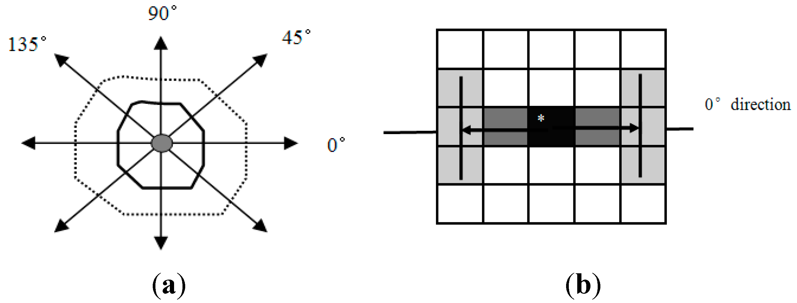
where $w_i(i=1,2,3)$ are weight coefficients, which are generally inversely proportional to the pixel distance to the detecting pixel, e.g., $w_1=w_3=0.2,w_2=0.6$. The four groups of formulae are, respectively, used to detect the local gray values of the minima points in the 0°, 45°, 90°, and 135° directions of the current detecting pixel. In Figure 4, the left diagram shows the four detection directions, where the area closed by the solid curve represents the first comparison region, the area closed by the dotted curve is the second comparison area; the right image shows the detection template in 0° direction, where the shadow parts are the pixels to be used for searching and comparing. The situations in other directions are similar to this.

Figure 4. Diagram for detection algorithm. (a) The four directions; (b) detection template in 0° direction of a froth image of large bubbles.

Figure 4. Diagram for detection algorithm. (a) The four directions; (b) detection template in 0° direction of a froth image of large bubbles.

For an image of non-large bubbles, we search for the local gray value minima points in a 3 × 3 kernel, and the above judgment conditions are simplified as:

$$f(i,j-1)\ge f(i,j)\le f(i,j+1)$$

(5)

$$f(i+1,j-1)\ge f(i,j)\le f(i-1,j+1)$$

(6)

$$f(i-1,j)\ge f(i,j)\le f(i+1,j)$$

(7)

$$f(i-1,j-1)\ge f(i,j)\le f(i+1,j+1)$$

(8)

If one of the conditions is satisfactory, the detected point is marked as an edge point, that is to set $g(i,j)=255$, and its location and direction are also marked; otherwise, go to Step 2.

Step 2, for all images, we identify whether the current detecting pixel is a local gray value minima point in a 5 × 5 kernel. It is similar to step 1 but with a set of different conditions. This step is applied to extract the edge point in which the gray value is equal to that in another point in its neighborhood region. The judgment conditions are illustrated as:

$$f(i,j-1)>f(i,j)=f(i,j+1)<f(i,j+2)$$

(9)

$$f(i+1,j-1)>f(i,j)=f(i-1,j+1)<f(i-2,j+2)$$

(10)

$$f(i+1,j)>f(i,j)=f(i-1,j)<f(i-2,j)$$

(11)

$$f(i+1,j+1)>f(i,j)=f(i-1,j-1)<f(i-2,j-2)$$

(12)

$$f(i,j+1)>f(i,j)=f(i,j-1)<f(i,j-2)$$

(13)

$$f(i-1,j+1)>f(i,j)=f(i+1,j-1)<f(i+2,j-2)$$

(14)

$$f(i-1,j)>f(i,j)=f(i+1,j)<f(i+2,j)$$

(15)

$$f(i-1,j-1)>f(i,j)=f(i+1,j+1)<f(i+2,j+2)$$

(16)

where, the first four formulae are utilized to detect the local gray value minima points, respectively, in 0°, 45°, 90°, and 135° directions of the current detecting pixel, and the rest four formulae are used in the reverse directions 180°, 225°, 270° and 315°, respectively.

If one of the above conditions is met, the detected point is marked as an edge point, i.e., set $g(i,j)=255$, and its location and direction is also marked.

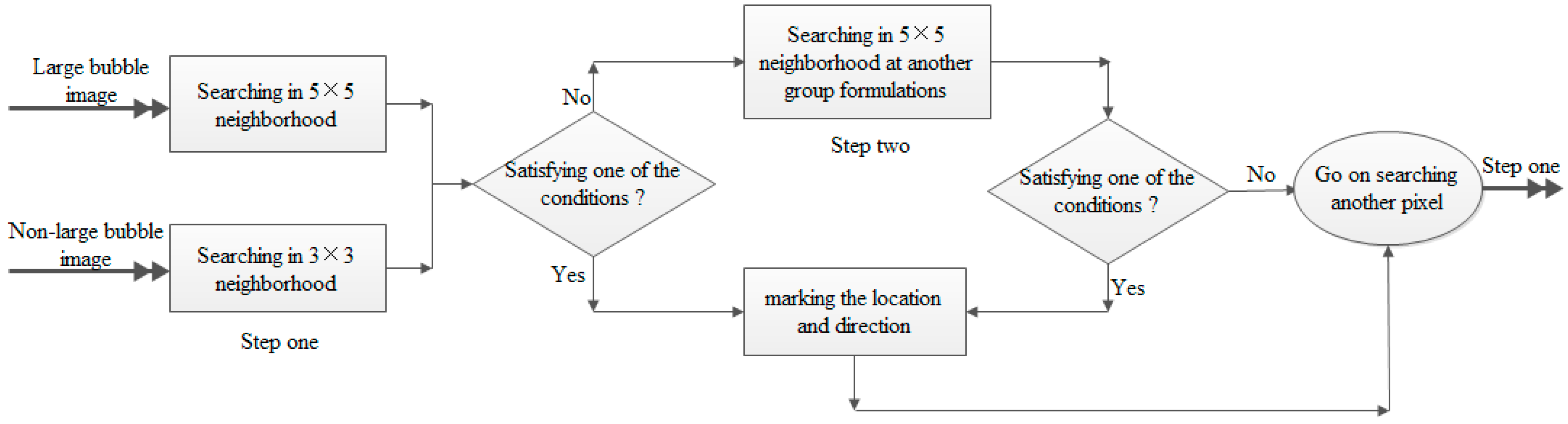
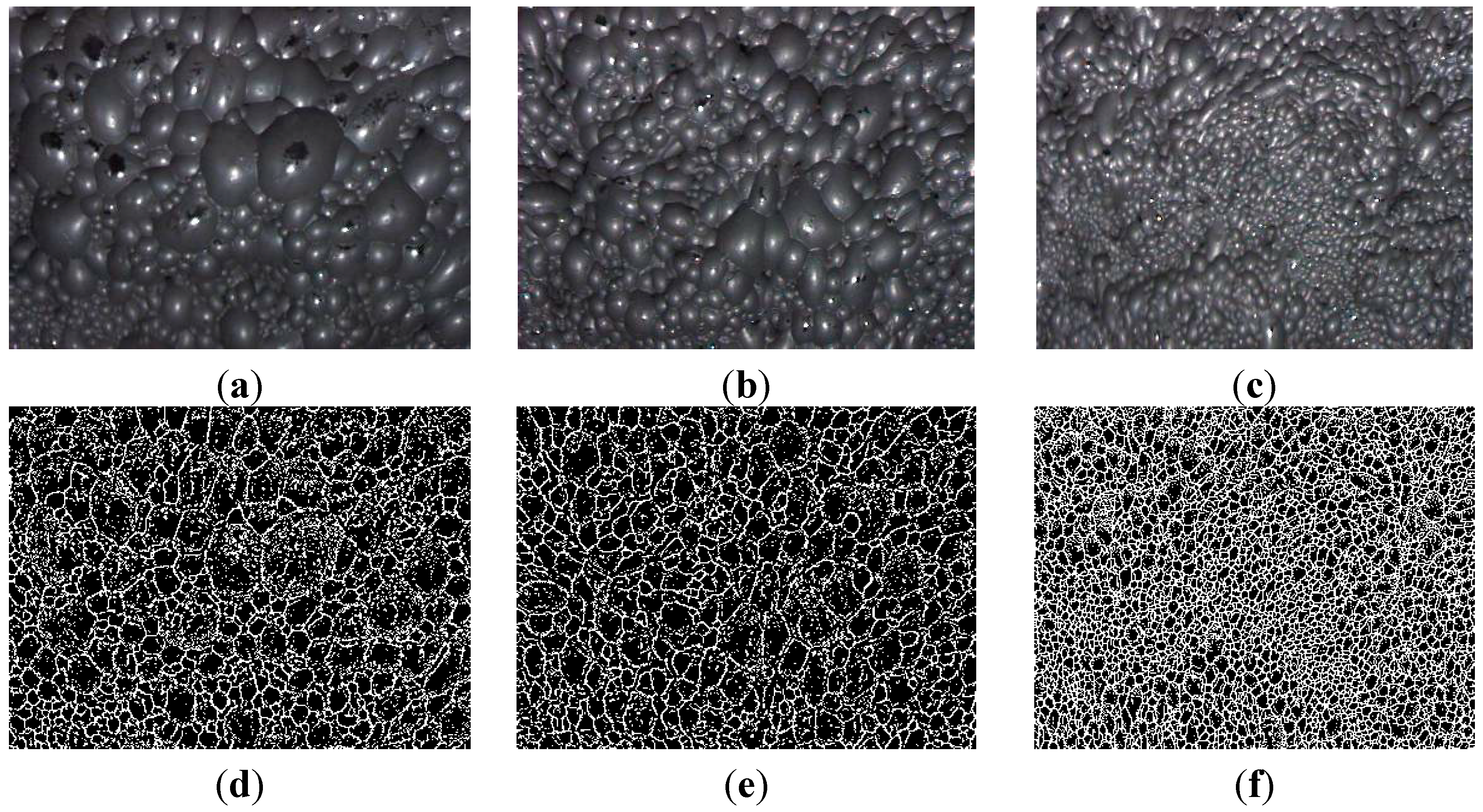
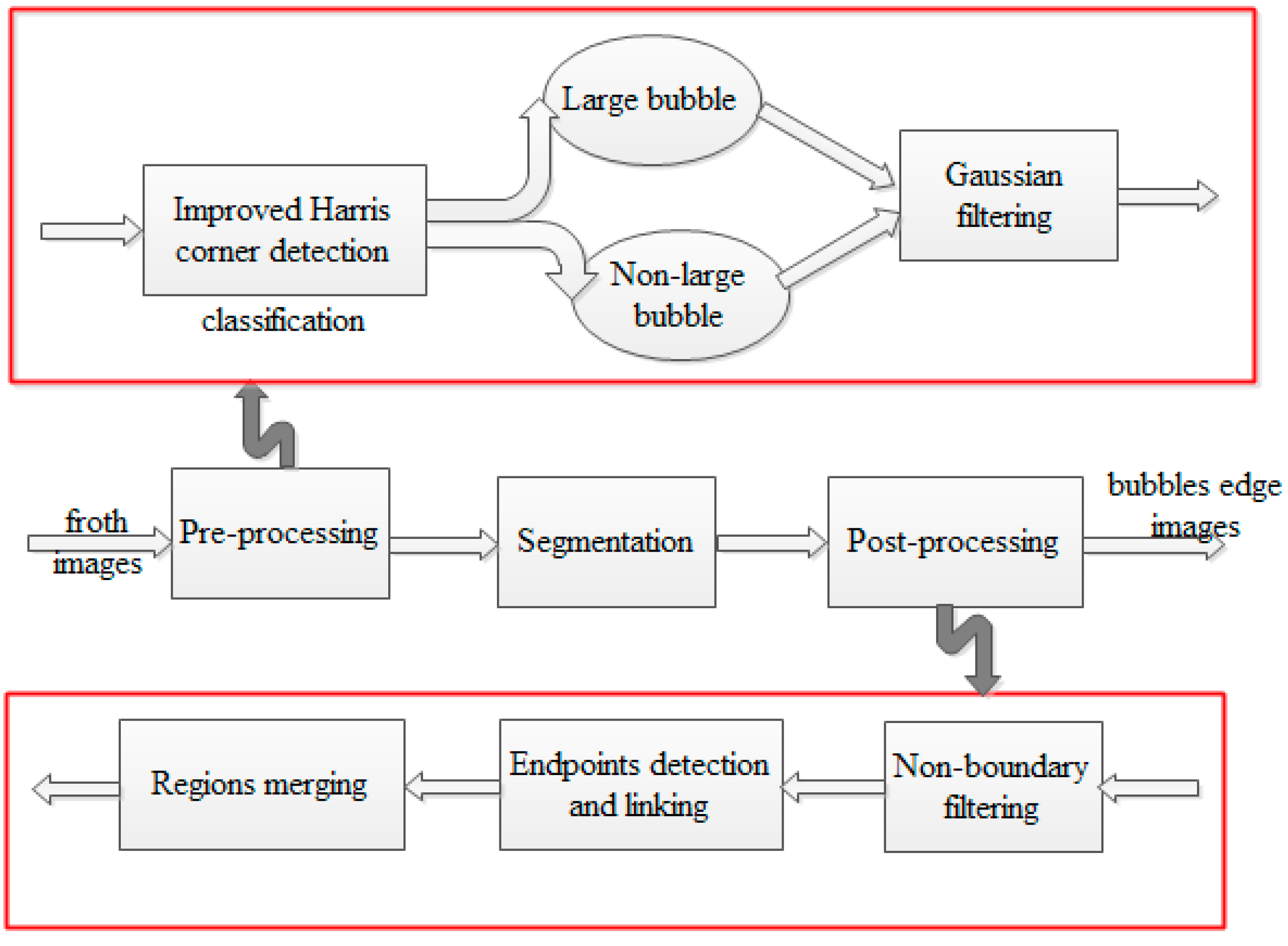
In accordance with the above-described detection method, each pixel in an image is detected to see if it is a local minima point in a certain direction. Any pixel having the local gray value minima in a certain direction is assigned as an edge point. It is noted that the edge point detection procedure is done after image classification. Figure 5 gives the workflow of the edge detection algorithm. The edge detection results for different classes of bubble images are shown in Figure 6.

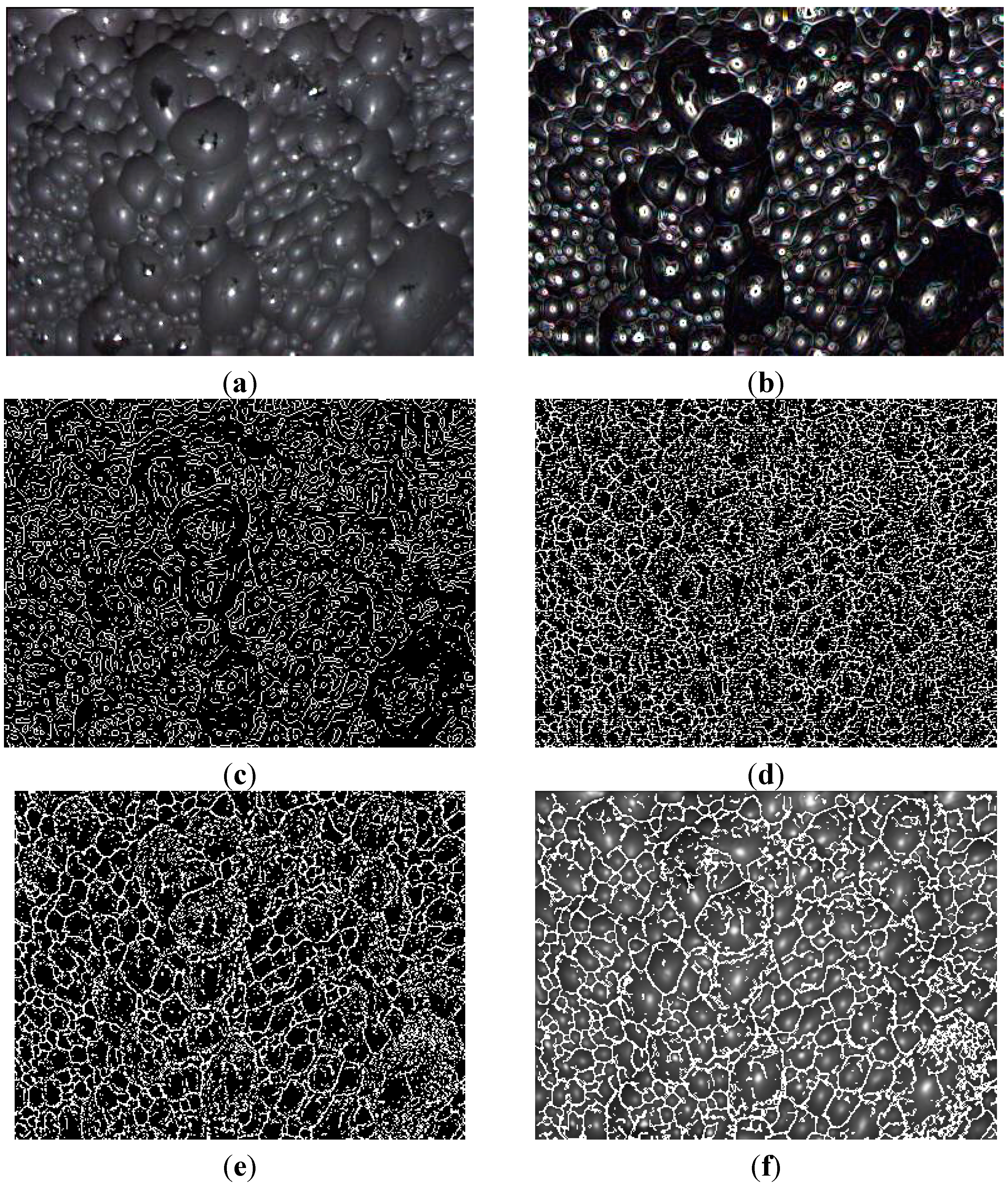
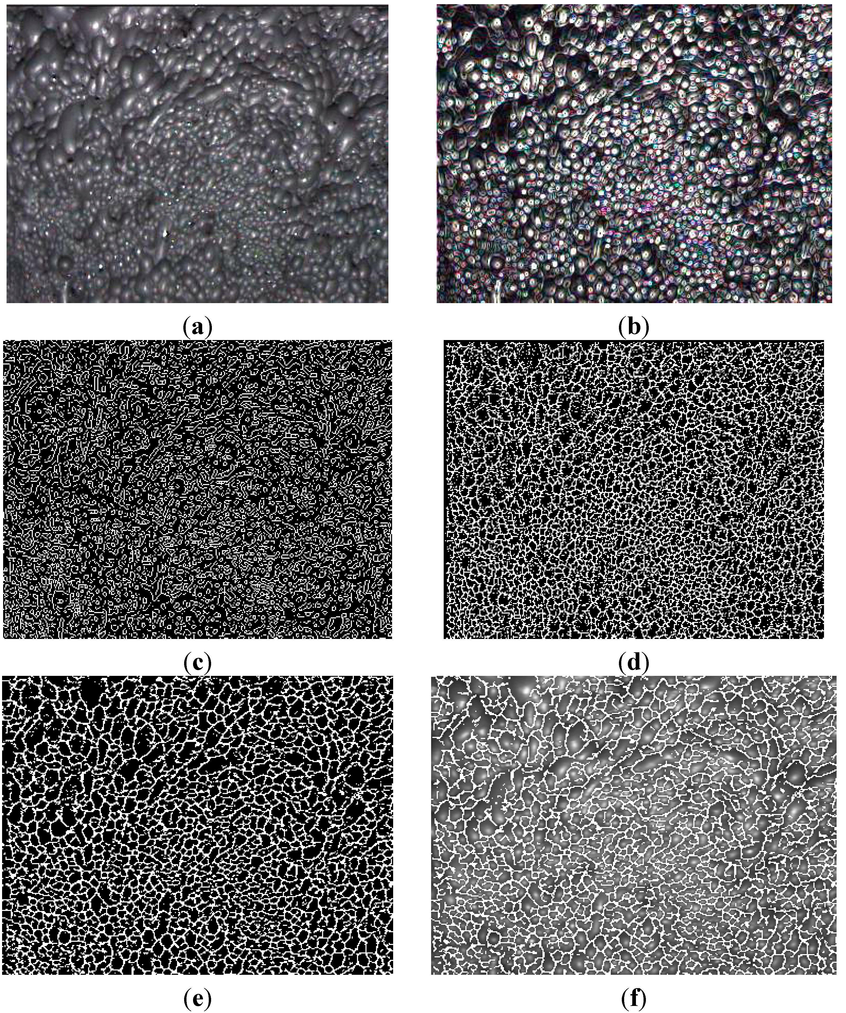
As shown in Figure 6, we can see that the significant bubble edges are detected and most of the white spot edges are eliminated for any class of bubble images. Those isolated points, short line segments, and other non-boundary information are removed in the subsequent post-processing procedures.

Figure 5. Algorithm workflow of the edge detection based on local gray value minima.

Figure 5. Algorithm workflow of the edge detection based on local gray value minima.

Figure 6. Edge detection results based on the proposed algorithm. (a–c) represent the original images of large, middle and small bubbles separately; (d–f) are the edge detection results corresponding to the images in (a), (b) and (c), respectively.

Figure 6. Edge detection results based on the proposed algorithm. (a–c) represent the original images of large, middle and small bubbles separately; (d–f) are the edge detection results corresponding to the images in (a), (b) and (c), respectively.

2.3. Image Pre-Processing and Classification

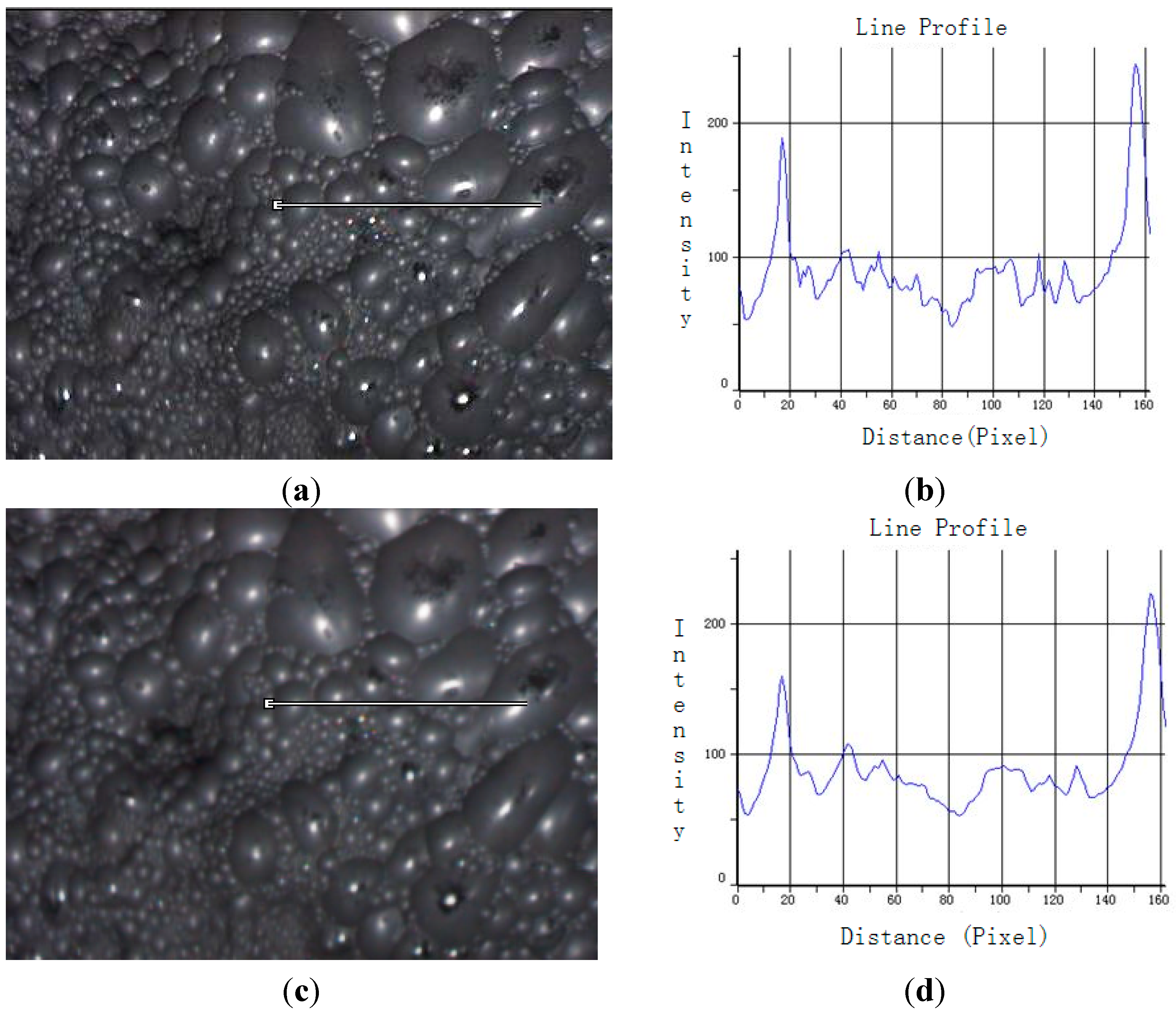
In general, there are a lot of noise in an original froth image, which makes the froth surface complicated. The noise might be detected as local gray value minima points to be reserved for they satisfy some conditions. So we need to smooth an original image to alleviate the noise before image segmentation. One simple way to reduce noise is to use a smoothing filter such as a mean filter or a Gaussian filter, and the de-noising procedure can be done before segmenting the classified froth images. Figure 7 shows the images smoothed by a Gaussian filter, from which we can see that the gray value variance in the image is more even after filtering, and it benefits the subsequent edge extraction procedures based on the local gray value minima.

Another preprocessing task is to classify these froth images according to bubble sizes. We have done a lot about the froth image classification with statistical analysis as shown in the reference [15]. Its statistical data have proven the following two facts: One is that the size of the white spot area on a bubble is proportional to the bubble size; the other is that the number of white spots in an image is inversely proportional to the average bubble size. In this study, we do image classification based on the latter. In order to extract the white spots in an image, many traditional threshold algorithms, such as Otsu threshold [24], can be used. As well known, the Otsu threshold algorithm is an automatic threshold segmentation method with the good performance for images having a obvious threshold between objects and background, but it is ineffective for the images having the unclear background, for example, for the images of small and tiny bubbles, the white spots are too small or of low gray values, therefore, it cannot effectively extract the white spots well. Moreover, after image segmentation, the region labeling and area size calculation must be carried out to calculate the number and the size distribution of white spots. To alleviate the problems of the Otsu threshold algorithm and to further simplify the image classification, this paper uses a corner detection method to conveniently get the number of white spots to do the bubble image classification.

Figure 7. Gray value variance comparison before and after Gaussian filtering. (a) Original froth image and a profile line; (b) Gray value histogram of the profile corresponding to the image (a) from left to right; (c) Result smoothed by the Gaussian filter and profile line at the same position; (d) Gray value histogram of the profile corresponding to the image (c) from left to right.

Figure 7. Gray value variance comparison before and after Gaussian filtering. (a) Original froth image and a profile line; (b) Gray value histogram of the profile corresponding to the image (a) from left to right; (c) Result smoothed by the Gaussian filter and profile line at the same position; (d) Gray value histogram of the profile corresponding to the image (c) from left to right.

A corner point contains the information of the image gray changes. Generally, it is believed that the corner point is the point of a maximum curvature value or a drastic change of the brightness in an image. These points not only retain the important image features but also effectively reduce the amount of data, which can improve the computation speed. A corner point plays a very important role in motion estimation, target tracking, image matching, and others in computer vision. In a froth image, the white spots of bubbles are the areas with a drastic intensity change, which is consistent with the definition of the corner point. Thus, the white spots can be obtained through a corner point detection method, and the number of corner points represents the number of white spots.

At present, the corner detection algorithms can be divided into three types: they are based on gray-scale images, the binary image and the contour curve, respectively. Harris corner detection algorithm is a gray level image corner detection method based on a template [25]. The algorithm detects the gray value change in the neighborhood of the detected pixel, and defines the pixel as a corner point when the change is large enough.

We now give a brief mathematical expression of the Harris corner detection algorithm. Denoting the image intensities by I, and the window function by $w(x,y)$, the window function is operated on the image pixel by pixel to detect the gray level change. The change E produced by a shift (u,v) is given by:

$$E(u,v)={\displaystyle \sum _{x,y}w(x,y){[I(x+u,y+v)-I(x,y)]}^2}={\displaystyle \sum _{x,y}w(x,y){[I_{x}u+I_{y}v+O(u^2,v^2)]}^2}$$

(17)

where, $I_x$, $I_y$ specify the first gradient results in x, y directions, respectively. It uses the Gaussian equation as the window function:

$$w(x,y)=\exp [-\frac{(x^2+y^2)}{2{\text{σ}}^2}]$$

(18)

The change E, for the small shift (u,v), can be concisely written as:

$$E(u,v)\cong {\displaystyle \sum _{x,y}w(x,y)[}{I_{x}u+I_{y}v]}^2={\displaystyle \sum _{x,y}w(x,y)[}u,v]\left[\begin{array}{cc}{I_x}^2& I_x{I}_y\\ I_x{I}_y& I_y^2\end{array}\right]\left[\begin{array}{c}u\\ v\end{array}\right]=[u,v]M\left[\begin{array}{c}u\\ v\end{array}\right]$$

(19)

where, M is a 2 × 2 symmetric matrix, and it can be written as:

$$M={\displaystyle \sum _{x,y}w(x,y)}\left[\begin{array}{cc}{I}_x^2& I_x{I}_y\\ I_x{I}_y& I_y^2\end{array}\right]$$

(20)

where, M can be made as a diagonalization matrix:

$$M\to R^{-1}\left[\begin{array}{cc}{\mathrm{\lambda }}_1& 0\\ 0& {\mathrm{\lambda }}_2\end{array}\right]R$$

where ${\mathrm{\lambda }}_1$ and ${\mathrm{\lambda }}_2$ are the eigenvalues of M, they are proportional to the principal curvatures of the local auto-correlation function, and form a rotationally invariant description of M.

Define the following formulation for the corner response function R:

$$R={\mathrm{\lambda }}_{\text{1}}{\mathrm{\lambda }}_2-k{({\mathrm{\lambda }}_1+{\mathrm{\lambda }}_2)}^2$$

(21)

where, k is an empirical constant, usually k is in the range of 0.04–0.06. R is positive in the corner region, negative in the edge region, and small in the flat region.

The Harris corner point detection algorithm is to compare the corner response function R with a threshold value given in advance. If R is greater than the threshold, then the pixel is marked as a corner point. In the improved Harris corner detection algorithm, the corner point determination condition is changed as: in the two eigenvalues, if the smaller one is greater than a given threshold, the pixel is determined as a corner point. In the mean time, the improved algorithm sets another tolerance distance parameter; in the given tolerance distance it only retains a strong corner point. By setting the reasonable tolerance distance parameter, the improved Harris corner detection algorithm is more suitable for being used to extract the white spots for image classification, and the calculation is simple.

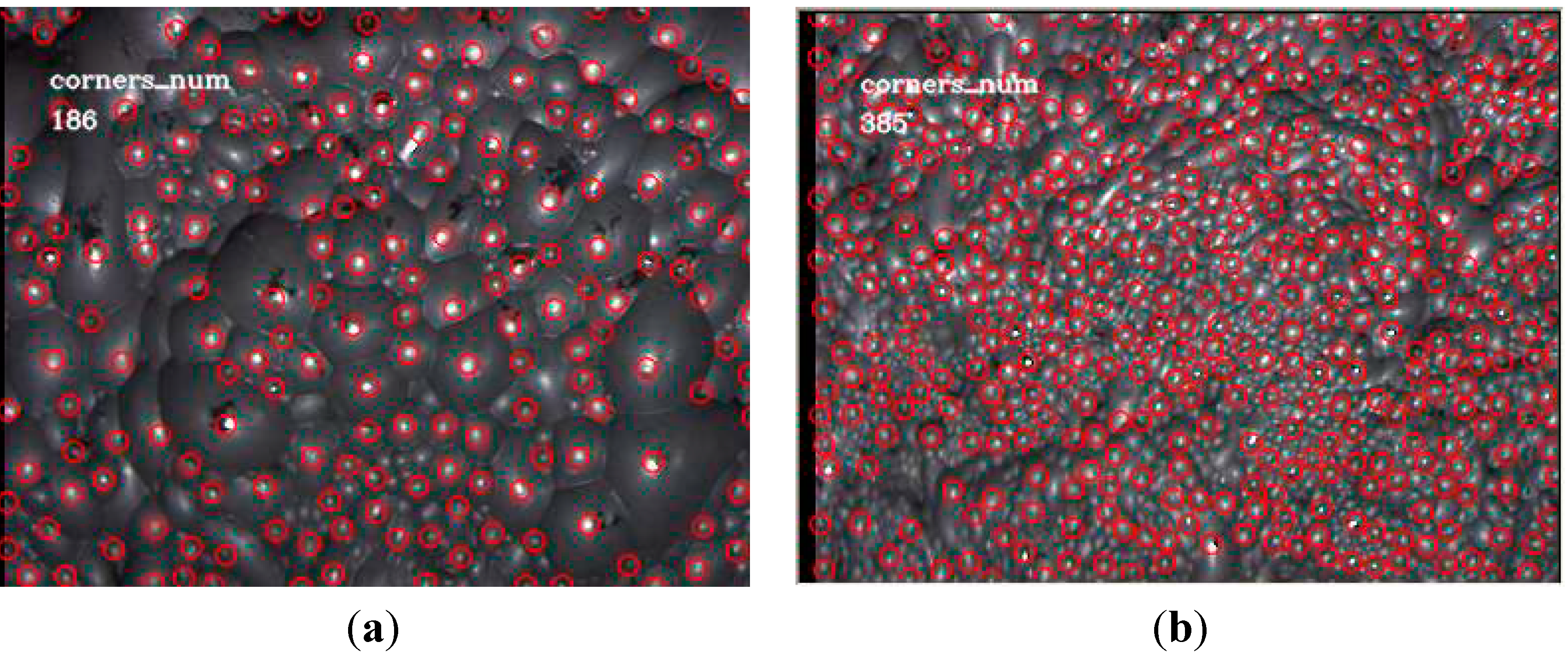
The extraction results of the corner points both in an image of large bubbles and in an image of small bubbles are shown in Figure 8. As we can see, most of the white spots are successfully marked as the corner points. Although there exist some false detection points and some white spots are missed, which only account for a small proportion, it does not affect obtaining the accurate image classification result.

Figure 8. Improved Harris corner point detection. (a) Result of the large bubbles with tolerance distance 15; (b) Result of the small bubbles with tolerance distance 11.

Figure 8. Improved Harris corner point detection. (a) Result of the large bubbles with tolerance distance 15; (b) Result of the small bubbles with tolerance distance 11.

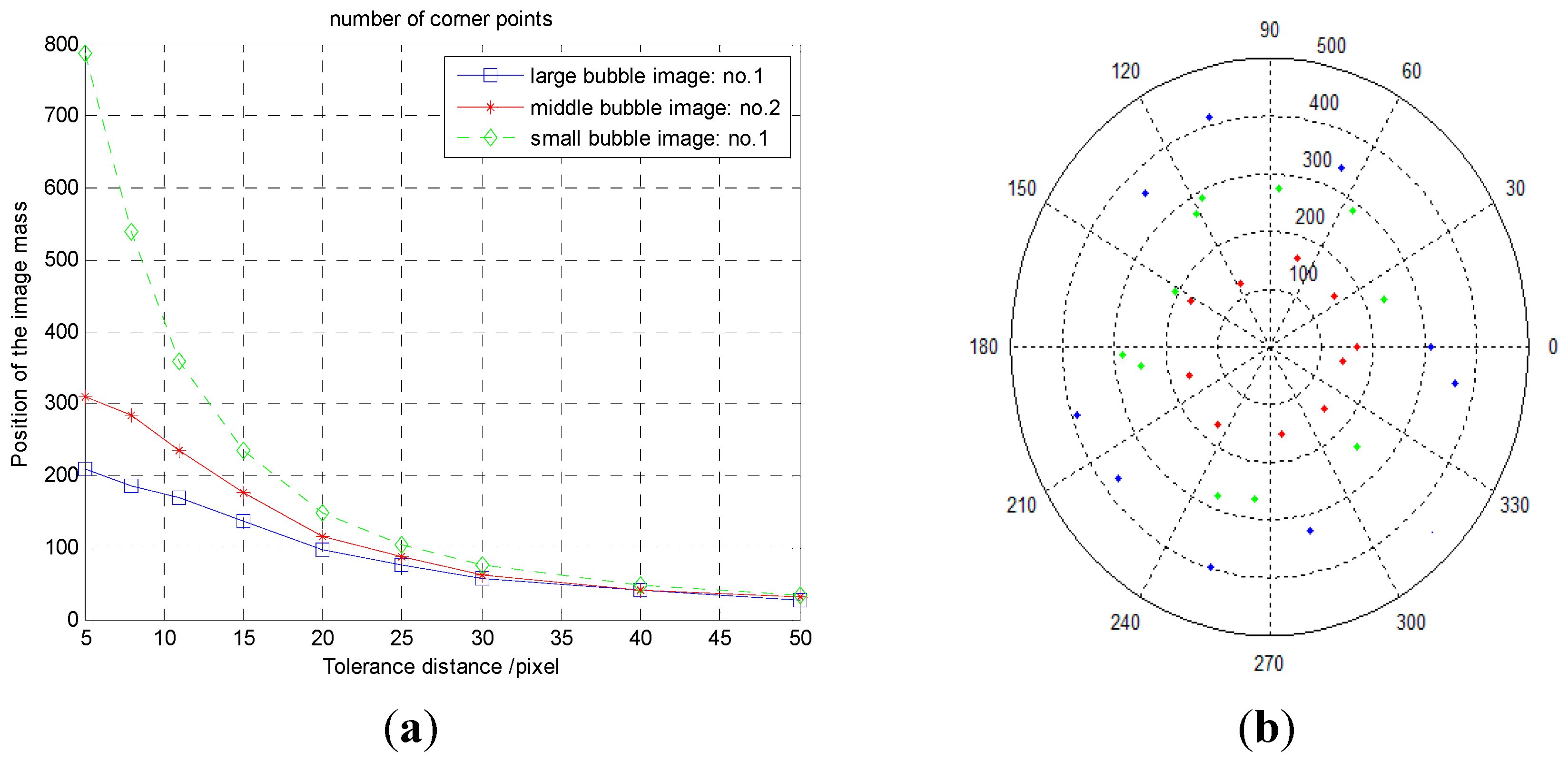
As an illustrative example, we choose six bubble images randomly to do the corner point detection. The six images, of size 384 × 288, are easily distinguished as the images of large, middle and small bubbles, and two of them are of large bubbles, two are of middle and the rest are of small bubbles. Table 1 shows the basic data and classification information, and the corresponding corner point number distribution is shown in the left of Figure 9.

From Table 1, we see that, with the tolerance distance decreasing, the changes of the numbers of the corner points in the different bubble images are growing more and more. With tolerance distance 40, the difference of the numbers of the three bubble images is little; with tolerance distance 8, the difference is great. With the distance 11, the corner point numbers in the images of small and middle bubbles are both above 200 and the numbers in the images of large bubbles are still below 200.

To verify the above general discipline, with the threshold 5 and the tolerance distance 11 pixels, we do the further test on 10 images of large bubbles and 20 images of middle, small and tiny bubbles, the specific data are shown on the right of Figure 9, where, the red dots represent the number of the corner points in the images of large bubbles, the green dots represent the images of middle and small bubbles, and the blue dots are for the images of tiny bubbles. The data distribution illustrates that the mentioned classification rule is feasible. Based on the above data analyses, we obtain the classification rules as follows: with the threshold 5 and the tolerance distance 11 pixels, if the number of corner points is above 200, the image belongs to that of non-large bubbles (the images of small, tiny and middle bubbles); otherwise, it belongs to that of large bubbles.

Figure 9. Corner point numbers (white spot numbers) distribution. (a) Corner point number distribution from Table 1; (b) Corner point number distribution of 30 different types of bubble images.

Figure 9. Corner point numbers (white spot numbers) distribution. (a) Corner point number distribution from Table 1; (b) Corner point number distribution of 30 different types of bubble images.

Table 1. Classification analysis based on the number of corner points (threshold of corner point detection algorithm is 5).

Tolerance Distance (Pixel)	Large Image No. 1	Large Image No. 2	Middle Image No. 1	Middle Image No. 2	Small Image No. 1	Small Image No. 2
5	210	200	269	310	787	677
8	187	176	249	284	539	470
11	169	164	213	236	359	372
15	138	136	162	176	234	213
20	97	106	113	115	148	134
25	75	80	80	88	104	103
30	58	56	63	63	77	74
40	41	38	42	41	49	47
50	27	30	28	31	35	32

Table 1. Classification analysis based on the number of corner points (threshold of corner point detection algorithm is 5).

Tolerance Distance (Pixel)	Large Image No. 1	Large Image No. 2	Middle Image No. 1	Middle Image No. 2	Small Image No. 1	Small Image No. 2
5	210	200	269	310	787	677
8	187	176	249	284	539	470
11	169	164	213	236	359	372
15	138	136	162	176	234	213
20	97	106	113	115	148	134
25	75	80	80	88	104	103
30	58	56	63	63	77	74
40	41	38	42	41	49	47
50	27	30	28	31	35	32

2.4. Post-Processing after Image Segmentation

After the image classification and the local gray value minima detection, most significant bubble edges exist in the magnitude gradient image. But the result image may not be satisfactory, because there are some isolated points, short line segments and small closed curves caused by noise, and some bubble edges are discontinuous. In order to overcome the problems, we have to do a number of post operations. Our post-processing subroutines include noise filtering, thinning, endpoint detection and gap linking, and region merging.

The isolated points and some short line segments with 2–3 pixels can easily be removed by some common filtering operators. For the images of small and middle bubbles, the non-boundary information is little, and after filtering the edge image for 3–4 times, the isolated points, the short line segments and other non-boundary points can almost be removed. For the images of large bubbles, the filtering steps should be done more times to remove the noise effectively.

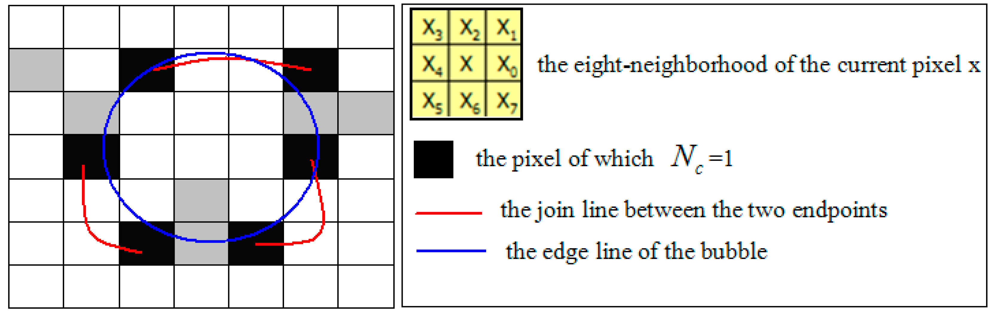
Before the edges are further thinned into of a width of one pixel, the simple noise filtering is performed. The last task is to make the closed bubble boundaries, which is done by endpoint detection and gap linking. We use the connection number of the detecting pixel to determine if the pixel is an endpoint. The connection number, $N_c$, is calculated by the following formula:

$$N_c={\displaystyle \sum _{k=0,2,4,6}[(1-f(x_k))}-(1-f(x_k))(1-f(x_{k+1}))(1-f(x_{k+2}))]$$

(22)

where $x_k$ denotes No. k pixel of the eight-neighborhood of the detecting pixel, as shown in Figure 10; and $f(x_k)$ represents the gray value of pixel $x_k$, where we define: $f(x_k)=1$ when the pixel is a white point (edge point), and $f(x_k)=0$ when the pixel is an non-edge point; and when $x_k=x_8$, we define $x_8=x_0$.

For each edge point, the connection number $N_c$ is calculated. When $N_c$=1, the detected edge point is marked as an endpoint, and both its direction and location are marked.

Figure 10. Gap linking diagram between the two endpoints and the representation of the pixels in the eight-neighborhood of the detecting pixel x.

Figure 10. Gap linking diagram between the two endpoints and the representation of the pixels in the eight-neighborhood of the detecting pixel x.

When all the endpoints are marked, the next step is to link the endpoints based on the principle of the similar direction and the nearest distance. We search for another endpoint in its 5 × 5 kernel as the detected endpoint as center. When a new endpoint is found, and its direction is the same to that of the detected endpoint, the new endpoint is linked along the direction to the current endpoint. When the direction is different, we choose the endpoint with the shortest distance to link along the direction of the current endpoint. When there is no endpoint to be found, then it skips the current endpoint and processes the next endpoint.

Through this procedure, there are some short line segments left. We use a line threshold to remove these false edges. The algorithm of Region merging is also used to remove some complex closed curves.

3. Experimental Results and Discussions

According to the above analyses, the workflow of the proposed method is given in Figure 11. It includes the following key steps:

(1)

Applying the improved Harris corner detection method to extract the white spots and calculate the total number of white spots. When the number is less than 200, the image is that of large bubbles; otherwise, it belongs to that of non-large bubbles.

(2)

Using the Gaussian filter to smooth the classified bubble image.

(3)

Taking advantage of the improved local gray value minima detection method to identify the minima point for each pixel to generate the binary edge image, where a 5 × 5 template is used for the images of large bubbles, and a 3 × 3 template for the images of non-large bubbles.

(4)

Carrying out the non-boundary information filter processing for the binary edge image to remove the isolated points and short line segments.

(5)

Adopting endpoint detection and gap linking, region merging and other operations to obtain the last edge image.

(6)

Overlapping the last edge image on the original bubble image.

Based on the above procedure, it can automatically complete the classification, edge detection, segmentation and bubble delineation in a froth image.

Figure 11. Working procedure of the proposed method.

Figure 11. Working procedure of the proposed method.

Figure 12e and Figure 13e give the result images only after the edge detection processing, respectively for the image of large bubbles and the image of non-large bubbles. For the comparison, we also test other edge detection algorithms including Valley-edge [15], Sobel and Canny [26,27]. In Figure 12, the images in (b–d) are the detection results of an image of large bubbles by using Sobel, Canny and Valley-edge respectively, and in Figure 13, the images in (b–d) are the corresponding detection results of an image of non-large bubbles.

As we can see in Figure 12 and Figure 13, the Sobel edge detection operator can only obtain some parts of the edges of bubbles regardless of which class of images, and what is more, the bubble edges are much weaker than the white spot edges. The same result is also obtained by the Canny operator, which lost most of the bubble edges. The above results illustrate that the classic edge detection algorithms fail to segment the bubble images, therefore the result edge (or gradient) images are difficult to be used for the further bubble delineation. Comparing to the results of Sobel and Canny operators, the Valley-edge detection algorithm and the proposed algorithm both produce the better results, where most significant bubble edges are detected and most white spot edges are disregarded. On the contrast, the proposed algorithm can obtain more bubble edge information than the Valley-edge detection algorithm.

Figure 12. Comparison between the proposed edge detection algorithm and others (for the image of large bubbles). (a) Original image; (b) Sobel result; (c) Canny result; (d) Valley-edge result; (e) New algorithm result; (f) Result of overlap (e) and (a).

Figure 12. Comparison between the proposed edge detection algorithm and others (for the image of large bubbles). (a) Original image; (b) Sobel result; (c) Canny result; (d) Valley-edge result; (e) New algorithm result; (f) Result of overlap (e) and (a).

After edge detection by the improved local gray value minima algorithm, the post-processing procedures can be done on the froth edge images to obtain the final good image segmentation results. The final segmentation results by the proposed algorithm are shown in the sixth row in Figure 14. We can see that the segmentation results are promising for all classes of froth images, compared with the other image segmentation algorithms based on the gray value similarity. In Figure 14, the four images in the first row are the original images, respectively, representing the images of large, middle, small and mixed-size bubbles; the four images in the second and the third rows show the optimal and Otsu global thresholding results, respectively, where most white spots are delineated, then most bubble edges are lost; the four images in the fourth and fifth rows are the segmentation results of the region growing algorithm with different thresholds, and we can see that the results are also not good. These algorithms based on local or global gray value similarity fail to produce satisfactory segmentation results because the gray values are different both in the interior of a bubble and in different areas in an image.

Figure 13. Comparison between the proposed edge detection algorithm and others (for the image of non-large bubbles). (a) Original image; (b) Sobel result; (c) Canny result; (d) Valley-edge result; (e) New algorithm result; (f) Result of overlap (e) and (a).

Figure 13. Comparison between the proposed edge detection algorithm and others (for the image of non-large bubbles). (a) Original image; (b) Sobel result; (c) Canny result; (d) Valley-edge result; (e) New algorithm result; (f) Result of overlap (e) and (a).

Figure 14. Comparison between the proposed algorithm and the algorithms based on gray value similarity: The first row is for the original images; the second row is for the segmentation results of the optimal threshold algorithm; the third row is for the results of Otsu threhsolding; the fourth and the fifth rows are for the results of the region growing algorithm with the threshold 30 and 35 separately; the sixth row is for the results of the proposed algorithm; the last row is for the results of manual delineation.

Figure 14. Comparison between the proposed algorithm and the algorithms based on gray value similarity: The first row is for the original images; the second row is for the segmentation results of the optimal threshold algorithm; the third row is for the results of Otsu threhsolding; the fourth and the fifth rows are for the results of the region growing algorithm with the threshold 30 and 35 separately; the sixth row is for the results of the proposed algorithm; the last row is for the results of manual delineation.

Our image segmentation algorithm produces the better results as shown in the four images of the sixth row in Figure 14, where, most bubbles are delineated correctly in each class of images. Even for the small bubbles between the large bubbles and the single large bubble in the small bubbles, the segmentation results are satisfactory although the under-segmentation problem still exists. We also note that it encounters the over-segmentation problem for the images of large bubbles in the mixed-size bubbles, and the black holes in the interior of a large bubble lead to the same problem.

In order to provide a quantitative comparison, we delineate the rest of bubbles manually based on the rough segmentation result of the Watershed algorithm and count the number of bubbles. The manual results are shown in the last row in Figure 14. Table 2 gives the data about the number of bubbles. The numbers are counted based on the results of our algorithm and manual separately.

Table 2. Bubbles numbers comparison between our algorithm and manual segmentation.

Froth Image Type	Large	Middle	Small	Mixed-Size
Manual segmentation	231	451	1537	500
Our algorithm	201	450	1799	472

Table 2. Bubbles numbers comparison between our algorithm and manual segmentation.

Froth Image Type	Large	Middle	Small	Mixed-Size
Manual segmentation	231	451	1537	500
Our algorithm	201	450	1799	472

We also make the comparison between the new algorithm and the Watershed algorithm; the results are shown in Figure 15, where the original images are the same as the image (a) in Figure 12 and Figure 13, respectively, representing the images of large bubbles or non-large bubbles. The commercial software, Image-pro Plus (version 6.0) (Media Cybernetics, Bethesda, MD, USA), is used to achieve the froth image segmentation result based on the Watershed algorithm. We set the gray value threshold in the Watershed algorithm, i.e., we separate objects using the gray levels (the preflooding level parameter) of the objects on the original image. The preflooding level parameter can be used to separate only slightly touching objects, avoiding separation of large objects.

Generally, the preflooding level can be set in a small value for small sized objects, and in a large value for the large sized objects. In Figure 15, images (a) and (c) are the Watershed segmentation results for the image of large bubbles, where the value of preflooding level is set as 20 and 40 separately; and the images in (b) and (d) are the segmentation results for the images of non-large bubbles, where the value of preflooding level is set as 1 and 5, respectively. When using the Watershed algorithm to segment a froth image, it is difficult to set a right adaptable parameter (preflooding level) to obtain a good result. For the image of large bubbles, a too small parameter value will cause the over-segmentation problem, as it can be seen in images (a) and (c); for the image of non-large bubbles, a too big value will lead to under-segmentation problem and also over-segmentation problem in some large bubbles, as shown in images (b) and (d). These results show that the segmentation results of the Watershed algorithm mainly depend on the appropriate parameter setting by manual. However, the parameter setting is hard and time-consuming for the reason that the parameter values differ greatly on different froth images. Obviously, the Watershed algorithm is difficult to be directly applied in an online froth analysis and monitoring system with a right parameter. On the contrary, the proposed method is a fully automatic processing procedure including image classification and image segmentation, in which it needs no manual operation. For the same images, the processing speed is tens to hundred times faster than the Watershed algorithm. Normally, for those froth images of size 384×288 pixels, it needs 0.05–0.1 s for processing one image on a PC (Inter Core 2.9 GHz), which makes the new method applicable in an online system.

Figure 15. Comparison between the proposed algorithm and the Watershed algorithm. (a) and (c) are for the Watershed segmentation results with preflooding level = 20, 40 separately for the image of large bubbles; (b) and (d) are for the Watershed segmentation results with preflooding level = 1, 5 separately for the image of non-large bubbles; (e) is for the image segmentation result by the proposed algorithm for the image of large bubbles; (f) is for the image segmentation result by the proposed algorithm for the image of non-large bubbles.

Figure 15. Comparison between the proposed algorithm and the Watershed algorithm. (a) and (c) are for the Watershed segmentation results with preflooding level = 20, 40 separately for the image of large bubbles; (b) and (d) are for the Watershed segmentation results with preflooding level = 1, 5 separately for the image of non-large bubbles; (e) is for the image segmentation result by the proposed algorithm for the image of large bubbles; (f) is for the image segmentation result by the proposed algorithm for the image of non-large bubbles.

4. Conclusions

This paper proposes a froth delineation method that is the combination of image classification and image segmentation. The corner detection algorithm is used to complete the image classification, and the improved local gray value minima algorithm is applied to achieve the image segmentation. The experimental results show that our method can produce good image segmentation results automatically and the processing speed is fast. The segmentation algorithm is to search the edge point located in a certain direction with gray value minima through the inequality comparison; therefore it is not affected by uneven illumination, bubble 3D geometry and other negative factors. In addition, the new image segmentation algorithm only do the logic comparative judgment without the complex numerical calculation, so the computing speed is fast and the method can meet the real-time requirements of the flotation production control in Jin Dong lead zinc flotation plant. The further improvement of the image segmentation algorithm is for the images of the mixed-size bubbles with many black holes. We will compare the proposed image segmentation algorithm at the industrial scale with the existing algorithms including the Watershed algorithm (used in SmartFroth) and others.