Long-Term Acid-Generating and Metal Leaching Potential of a Sub-Arctic Oil Shale

Abstract

Shales are increasingly being exploited for oil and unconventional gas. Exploitation of sub-arctic oil shales requires the creation of gravel pads to elevate workings above the heaving effects of ground ice. These gravel pads can potentially generate acidic leachate, which can enhance the mobility of metals from the shale. To examine this potential, pyrite-bearing shale originating from sub-Arctic gravel pad sites were subjected to leaching tests for 600 days at initial pH values ranging from 2 to 5, to simulate potential real world conditions. At set times over the 600 day experiment, pH, oxidation reduction potential (ORP), dissolved oxygen and temperature were recorded and small liquid samples withdrawn and analysed for elemental concentrations using total reflection X-ray fluorescence spectrometry (TRXRF). Six of eight shale samples were found to be acid generating, with pH declining and ORP becoming increasingly positive after 100 days. Two of the eight shale samples produced increasingly alkaline leachate conditions with relatively low ORP after 100 days, indicating an inbuilt buffering capacity. By 600 days the buffering capacity of all samples had been consumed and all leachate samples were acidic. TRXRF analyses demonstrated significant potential for the leaching of S, Fe, Ni, Cu, Zn and Mn with greatest concentrations found in reaction vessels with most acidic pH and highest ORP.

1. Introduction

Oil and gas drilling operations in Arctic and sub-Arctic regions often require extensive ground stabilization and construction of gravel pads above the tundra to host drilling equipment, accommodation modules and other buildings. The isolation and transportation costs to these areas effectively restricts “borrow” materials to what is available on or near site, which in sedimentary basins hosting hydrocarbons consists typically of limestone, siltstone and shale. Shale is generally characterised by high concentrations of sulfidic materials such as pyrite (FeS₂), which in the presence of air and sufficient water, are capable of being oxidized to iron sulfates and sulfuric acid [1]. Increased acidity combined with appropriate oxidation-reduction potential (ORP) conditions [2] allows for increased mobility and potential leaching of elements from otherwise stable materials. The elements leached at a particular location are a function of the local geology [3], however elements such as S, Mn, Fe, Cu, Zn, As, Se, Cd, Hg and Pb are common [4,5]. This process is generally referred to as acid rock drainage (ARD). ARD can cause significant environmental damage to many facets of ecosystems including aquatic life [5,6], vegetation [5,7] and groundwater [8]. These elements often bio-accumulate [9]. Many case studies evaluating ARD have been undertaken around the world [10,11,12,13], however, to date no studies have been undertaken on gravel construction pads in Arctic or sub-Arctic regions. As shale from gravel pads on oil and gas field sites in Canada is used in this study, Canadian Soil Guidelines will be used to evaluate the risks associated with ARD in this work.

The development of ARD can occur over long time scales and so a number of standard laboratory procedures, with varying degrees of complexity and accuracy, have been developed or adapted to forecast the potential for ARD and possible leachable metals. The most commonly used tests to quantify ARD potential are “static” tests and “kinetic” tests. The most common static test is acid-base accounting (ABA), which is a simple balance of the acid producing and acid neutralizing potential of a rock [14], and is used to determine whether or not a material is acid generating. Importantly, ABA does not account for the various dissolution rates of the constituent materials and hence does not provide a guide to the overall impact on site pH over time.

Full chemical digests of rocks are used to reveal contaminants present and their concentration. Often U.S. Environmental Protection Agency (EPA) Methods are used for this purpose, however as they have not been specifically designed for ARD conditions their applicability is uncertain. For instance, U.S. EPA method 1311 (Toxicity Characteristic Leaching Procedure) was designed to simulate co-disposal in municipal waste while U.S. EPA method 1312 (Synthetic Precipitation Leaching Procedure) was designed to simulate leaching by mildly acidic rain. Conversely, the strong acid leach test (SALT) was designed for ARD conditions [15]. The SALT involves the addition of sulfuric acid to a reaction flask in sufficient quantities to ensure a predetermined final pH irrespective of the buffering capacity of the material. However, similar to the U.S. EPA methods, the SALT contains no provision for the kinetics of ARD reactions as samples are collected and metal concentrations quantified at only one time interval.

Kinetic tests most commonly take the form of laboratory-based columns, humidity cells or field based test pads. These tests can be designed to provide useful information of the relative rates of acid generation and neutralisation as well as the drainage chemistry and resultant loadings downstream [16]. However, these tests do have limitations, specifically matching laboratory set points to site-specific factors such as water flow rates and dissolved oxygen concentrations. Differences in these key set points can result in significant variations between laboratory predictions and site outcomes [17].

This investigation combines features of static and kinetic tests, such that potential for ARD is characterised and the potential for metals to be leached quantified over time. Similar to the SALT method, a specific mass of rock is placed in a reaction vessel with a specified amount of water and pH adjusted to a value between 2 and 5 with sulfuric acid. Flasks are shaken at low speed and samples withdrawn at set intervals for 600 days with temperature, pH, ORP and metal concentrations measured. This procedure enables analysis of reaction kinetics without potential inconsistencies due to poorly selected water flow rates. However, due to the long time scale involved and increased ion concentrations in solution, this procedure does have the risk of being impacted by secondary mineral precipitation processes. The stability of these phases is potentially important in the control of metal distribution [18].

Due to the large number of samples required from each flask to provide adequate kinetic data this work uses a relatively new analytical procedure to quantify metal concentrations leached into solution, total reflection X-ray fluorescence spectrometry (TRXRF). TRXRF can quantify concentrations of elements from Na to U present in a sample down to µg/L levels, much lower than would typically be possible with other forms of XRF spectrometry [19]. Only approximately 1 mL is required per sample, much less than for flame atomic absorption spectroscopy (F-AAS) [20], inductively coupled plasma atomic emission spectroscopy (ICP-AES) [21], or inductively coupled plasma mass spectrometry (ICP-MS) [22]. Sector field ICP-MS was employed as an external analytical comparison method.

2. Materials and Methods

2.1. Sample Collection

Shale samples were collected from an oil and gas lease area in the Canadian Arctic. Sample locations were either in areas of high potential environmental risk, where large volumes of shale were present or collected from creek banks due to their direct contact with local aquatic ecosystems. Samples were collected from a depth of approximately 10 cm, and consisted of gravel (2–50 mm b-axis diameter). The samples were not sterilized, but the mineral fragments were free of soil and plant matter.

2.2. Sample Comminution

Samples of solids were oven dried at 60 °C for 48 h, then crushed without lubricant in a Rocklabs (Onehunga, New Zealand) Enerpac hydraulic crusher with tungsten carbide jaws (Model Number RR-308, 70 MPa pressure) and dry sieved to 0.5–2 mm diameter.

2.3. Material Characterisation

X-ray diffractometry (XRD) was used to identify the mineralogy of every crushed solid sample. X-ray diffractograms were collected with a PANalytical (Almelo, The Netherlands) X’Pert Pro MPD diffractometer, using 45 kV, 40 mA, Cu-Kα radiation and an X’Celerator detector. Scans were collected with 0.05° 2θ steps from 10° to 90° 2θ. Quantitative mineral identification was carried out using PANalytical X’Pert HighScore Plus version 2.2a software with patterns from ICDD PDF-2 and PAN-ICSD version 2008-2 (0.1–0.5 wt % detection limit). A PANalytical Epsilon 5 cartesian geometry energy dispersive XRF spectrometer was used to identify elemental concentrations in crushed shale from every sample. The Epsilon 5 XRF analysed samples in a vacuum, with a dual anode W/Sc tube, and six measurement conditions (Table 1). Measurements were made in triplicate and averaged. Elemental quantification was conducted using “Auto Quantify”, PANalytical’s automated qualitative spectrum analysis combined with a fundamental parameters model. All major element data are reported as oxides, and the analytical sum was set to 100%. Precipitates were not characterized at any time during the experiment, as the experiment focused solely on the leachate composition which is able to be discharged to the receiving environment. Precipitates, and any other solid phase, were immobile and not of interest for this experiment.

Table 1. Epsilon 5 XRF measurement conditions.

Elements	Secondary Target	Measurement Live Time (s)	Tube (kV)	Tube (mA)
Na-Mg	Al	200	35	17
Al-K	CaF2	200	40	15
Ca-Mn	Fe	100	75	8
Fe-Ga	Ge	100	75	8
Ge-Y	Zr	100	100	6
Zr-U	Al2O3 (Barkla)	100	100	6

Table 1. Epsilon 5 XRF measurement conditions.

Elements	Secondary Target	Measurement Live Time (s)	Tube (kV)	Tube (mA)
Na-Mg	Al	200	35	17
Al-K	CaF2	200	40	15
Ca-Mn	Fe	100	75	8
Fe-Ga	Ge	100	75	8
Ge-Y	Zr	100	100	6
Zr-U	Al2O3 (Barkla)	100	100	6

2.4. Sample Acidification and Leaching

Concentrated (98%) sulfuric acid (H₂SO₄) was diluted to a 4.9% solution with Type 1 (ASTM D1193-91) deionised water. The diluted acid was added to Type 1 deionised water in 500 mL HDPE square section wide mouth screw top containers in sufficient quantities to produce 350 mL of solution with a pH value of 2, 3, 4, or 5 (monitored with Hanna (Woonsocket, RI, USA) HI9025 microcomputer pH meter with HI1230 probe). 10.00 g of the prepared 0.5–2.0 mm gravel fraction of shale was placed into the prepared solutions, with a duplicate of each.

The prepared reaction vessels and blanks were placed on Ratek platform orbital mixers (Ratek Instruments (Boronia, Australia) Model OM7) operating at 100 rpm. Lids were screwed loosely onto the vessels so oxidising conditions could prevail. At set time intervals (1, 2, 4, 8 h, and 1, 2, 4, 21, 30, 100 and 600 days) 1.5–2 mL of sample was withdrawn from each reaction vessel using a 3 mL syringe, and air and solution temperatures (Hanna HI9025 microcomputer pH meter with temperature probe), pH, dissolved oxygen (DO, Hanna HI9142 Dissolved oxygen meter) and oxidation-reduction potential (Hanna HI9025 microcomputer pH meter with HI3230 ORP probe) was measured and recorded from each reaction vessel. The 1.5–2 mL sample was filtered using a 25 mm diameter 0.45 µm pore size cellulose acetate (“MiniSart”) syringe filter into a clean 6 mL HDPE intermediary vessel. 930 µL of sample was then withdrawn from each intermediary vessel and added to a 6 mL sample vial.

50 µL of 20.0 mg/L Gallium and Germanium standard solution (for TRXRF analysis) was added to every sample. 20 µL of concentrated nitric acid (HNO₃; 69%; AnalaR reagent grade) was also added to each sample vial to acidify samples to pH <2 and keep metals in solution. Every sample vial then contained 1.000 mL of sample spiked with 1.000 mg/L of Ga and Ge. The sample was then placed on a 2000 rpm vortex mixer for 3 s to ensure homogeneity of the solution. 10 µL of solution from every sample vial was pipetted onto a highly polished acrylic disc. This was then placed in a desiccator cabinet (containing silica gel) to allow the liquid to evaporate, leaving a residue on each disc for analysis. Some samples, especially blank and pH 2 samples, did not dry completely in the cabinet, and so were placed on a heating block at 60 °C to dry.

Samples were analysed using a Bruker (Berlin, Germany) S2 Picofox Total Reflection XRF spectrometer. Bruker Spectra software (version 7.0) was used to analyse spectra and derive concentrations of all elements present in samples, using the area of every peak present for all spectra. A multi-element calibration solution was used consisting of certified individual element solutions containing 10.0 mg/L of Ca, 1.00 mg/L of Cr, Fe, Ni, and Cu and 0.5 mg/L of Pb with detection limits <5 mg/kg. A gain correction disc containing 1 µg of arsenic was run every 5 discs to correct for any drift in the detector. At 21 days the first duplicate of each treatment was retired, and the remaining flasks continued to 600 days.

As an independent quality control 26 water samples, selected at random, were analysed for S, Ca, Cr, Mn, Fe, Co, Ni, Cu, Zn, Ga, As and Pb using sector field ICP-MS (ELEMENT 2, Thermo Fisher, Bremen, Germany) at the Central Science Laboratory, University of Tasmania. Three predefined instrumental resolution settings were employed to overcome spectral interferences commonly encountered for isotopes of mass ≤80 amu [23]. Elemental concentrations determined using TXRF and the more sensitive SF-ICP-MS were compared. Analytes with concentrations >50 µg/L had average differences of <5% (Fe, Ni, Cu, Zn), <10% (Mn) and <25% (S, Pb) (further detail may be found in the Supplementary Information).

3. Results

3.1. Material Characterisation

Shale samples were composed mainly of quartz and muscovite, with minor amounts of other minerals (feldspars, carbonates, sulfides and salts; Table 2). Shale B and C contained 11% and 6% anorthite, respectively. Shale H contained 4% orthoclase, and Shale D contained 3% halite. All samples had ~1% pyrite content, except for Shale C, which had <1%. Shale A also had ~1% marcasite, an iron sulfide similar to pyrite, with the same chemical formula (FeS₂), but different chemical structure. Marcasite oxidises more readily than pyrite [24], potentially making Shale A more acid-generating than other samples considered. Shales D and H contained 1% and 3% dolomite respectively, a mineral with pH buffering capacity, known to raise pH levels and reduce acidity [25]. As no other samples contained detectable dolomite, it is likely that Shale D, and particularly Shale H will have greater buffering capacity, potentially producing lesser acidic conditions than the other shales.

Elemental analyses indicate that shale samples were composed mostly of Si, followed by Al, Fe, K, Ca and Ti (Table 3), consistent with the shale mineralogy which is dominated by quartz and other silicates. Of greater interest are trace metals and metalloids of environmental significance. Table 4 presents the concentrations of a selection of these metals and compares them to the Canadian Soil Quality Guidelines for the Protection of Environmental and Human Health (agricultural) [26]. For all samples, concentrations of Cr, Cu, As, Se, V, Ni and Ba exceeded the agricultural Canadian Soil Guideline limit whilst Shale D and H exceeded the Zn soil guideline limit. All samples contained Pb concentrations below the soil guideline limit. Under acidic conditions, these elements have the potential to become soluble and leach, possibly posing a threat to local soil and aquatic ecosystems.

Table 2. Quantitative mineralogy (wt % abundance) from the shale samples using X-ray diffractometry. Blank cells indicate non-detection.

Shale	Major Minerals (Quartz SiO2, Muscovite KAl2(AlSi3O10)(F,OH)2)	Minor Minerals (Anorthite CaAl2Si2O8, Halite NaCl, Orthoclase KAlSi3O8)	Acidity-releasing minerals (Pyrite FeS2, Marcasite FeS2)	Neutralizing Minerals (Dolomite CaMg(CO3)2)
A	Quartz 46%, Muscovite 52%		Pyrite 1%, Marcasite 1%
B	Quartz 47%, Muscovite 42%	Anorthite 11%	Pyrite 1%
C	Quartz 45%, Muscovite 49%	Anorthite 11%	Pyrite <1%
D	Quartz 53%, Muscovite 43%	Halite 3%	Pyrite 1%	Dolomite 1%
E	Quartz 74%, Muscovite 25%		Pyrite 1%
F	Quartz 56%, Muscovite 44%		Pyrite 1%
G	Quartz 54%, Muscovite 45%		Pyrite 1%
H	Quartz 52%, Muscovite 40%	Orthoclase 4%	Pyrite 1%	Dolomite 3%

Table 2. Quantitative mineralogy (wt % abundance) from the shale samples using X-ray diffractometry. Blank cells indicate non-detection.

Shale	Major Minerals (Quartz SiO2, Muscovite KAl2(AlSi3O10)(F,OH)2)	Minor Minerals (Anorthite CaAl2Si2O8, Halite NaCl, Orthoclase KAlSi3O8)	Acidity-releasing minerals (Pyrite FeS2, Marcasite FeS2)	Neutralizing Minerals (Dolomite CaMg(CO3)2)
A	Quartz 46%, Muscovite 52%		Pyrite 1%, Marcasite 1%
B	Quartz 47%, Muscovite 42%	Anorthite 11%	Pyrite 1%
C	Quartz 45%, Muscovite 49%	Anorthite 11%	Pyrite <1%
D	Quartz 53%, Muscovite 43%	Halite 3%	Pyrite 1%	Dolomite 1%
E	Quartz 74%, Muscovite 25%		Pyrite 1%
F	Quartz 56%, Muscovite 44%		Pyrite 1%
G	Quartz 54%, Muscovite 45%		Pyrite 1%
H	Quartz 52%, Muscovite 40%	Orthoclase 4%	Pyrite 1%	Dolomite 3%

Table 3. Major element composition (wt % abundance) of the shale samples. Analyses were conducted on crushed solid fragments using X-ray fluorescence spectrometry.

Shale	Na2O	MgO	Al2O3	SiO2	S	K2O	CaO	TiO2	Fe2O3
Shale A	<1.0	<1.0	9.8	84.6	<1.0	1.15	0.68	0.30	2.46
Shale B	<1.0	<1.0	10.5	83.7	<1.0	1.29	0.54	0.32	2.66
Shale C	<1.0	<1.0	9.9	85.0	<1.0	1.12	0.69	0.28	2.00
Shale D	<1.0	<1.0	10.2	83.6	<1.0	1.12	1.53	0.28	2.19
Shale E	<1.0	<1.0	<0.1	96.4	<1.0	0.79	0.39	0.23	1.07
Shale F	<1.0	<1.0	9.4	86.0	<1.0	1.02	0.49	0.26	1.83
Shale G	<1.0	<1.0	9.5	85.6	<1.0	1.04	0.65	0.27	1.93
Shale H	<1.0	<1.0	13.1	77.5	<1.0	1.63	3.20	0.40	3.01

Table 3. Major element composition (wt % abundance) of the shale samples. Analyses were conducted on crushed solid fragments using X-ray fluorescence spectrometry.

Shale	Na2O	MgO	Al2O3	SiO2	S	K2O	CaO	TiO2	Fe2O3
Shale A	<1.0	<1.0	9.8	84.6	<1.0	1.15	0.68	0.30	2.46
Shale B	<1.0	<1.0	10.5	83.7	<1.0	1.29	0.54	0.32	2.66
Shale C	<1.0	<1.0	9.9	85.0	<1.0	1.12	0.69	0.28	2.00
Shale D	<1.0	<1.0	10.2	83.6	<1.0	1.12	1.53	0.28	2.19
Shale E	<1.0	<1.0	<0.1	96.4	<1.0	0.79	0.39	0.23	1.07
Shale F	<1.0	<1.0	9.4	86.0	<1.0	1.02	0.49	0.26	1.83
Shale G	<1.0	<1.0	9.5	85.6	<1.0	1.04	0.65	0.27	1.93
Shale H	<1.0	<1.0	13.1	77.5	<1.0	1.63	3.20	0.40	3.01

Table 4. Composition of selected trace elements (mg/kg). Canadian Soil Quality Guidelines (CSQG) for the Protection of Environmental and Human Health—Agriculture (2007) [26] are given where available. Concentrations above the CSQG are noted in the final row.

Shale	V	Cr	Mn	Ni	Cu	Zn	As	Se	Ba	Pb
Shale A	168	96	93	79	123	133	19	12	1827	38
Shale B	162	103	85	58	126	84	16	12	1890	43
Shale C	305	96	63	66	110	80	24	13	2150	31
Shale D	255	89	115	104	125	251	20	12	2069	30
Shale E	265	66	48	75	96	80	23	13	2051	<5
Shale F	249	82	72	94	113	146	17	13	1881	28
Shale G	198	82	76	102	106	152	20	15	2024	21
Shale H	289	116	205	163	144	244	34	16	2212	32
CSQG (mg/kg)	130	64	N/A	50	63	200	12	1	750	70
Sites failing CSQG	A-H	A-H	N/A	A-H	A-H	D, H	A-H	A-H	A-H	Nil

Table 4. Composition of selected trace elements (mg/kg). Canadian Soil Quality Guidelines (CSQG) for the Protection of Environmental and Human Health—Agriculture (2007) [26] are given where available. Concentrations above the CSQG are noted in the final row.

Shale	V	Cr	Mn	Ni	Cu	Zn	As	Se	Ba	Pb
Shale A	168	96	93	79	123	133	19	12	1827	38
Shale B	162	103	85	58	126	84	16	12	1890	43
Shale C	305	96	63	66	110	80	24	13	2150	31
Shale D	255	89	115	104	125	251	20	12	2069	30
Shale E	265	66	48	75	96	80	23	13	2051	<5
Shale F	249	82	72	94	113	146	17	13	1881	28
Shale G	198	82	76	102	106	152	20	15	2024	21
Shale H	289	116	205	163	144	244	34	16	2212	32
CSQG (mg/kg)	130	64	N/A	50	63	200	12	1	750	70
Sites failing CSQG	A-H	A-H	N/A	A-H	A-H	D, H	A-H	A-H	A-H	Nil

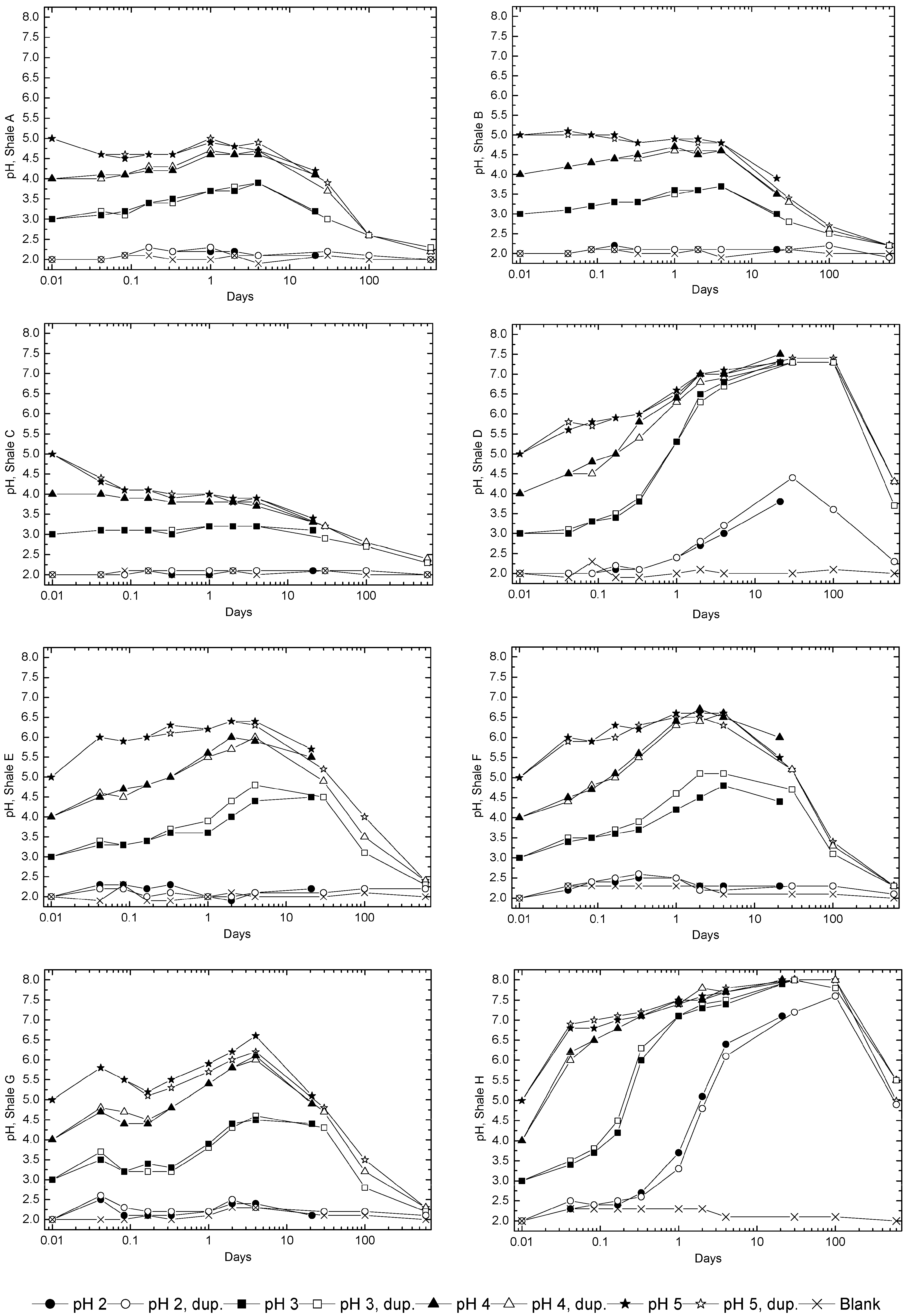
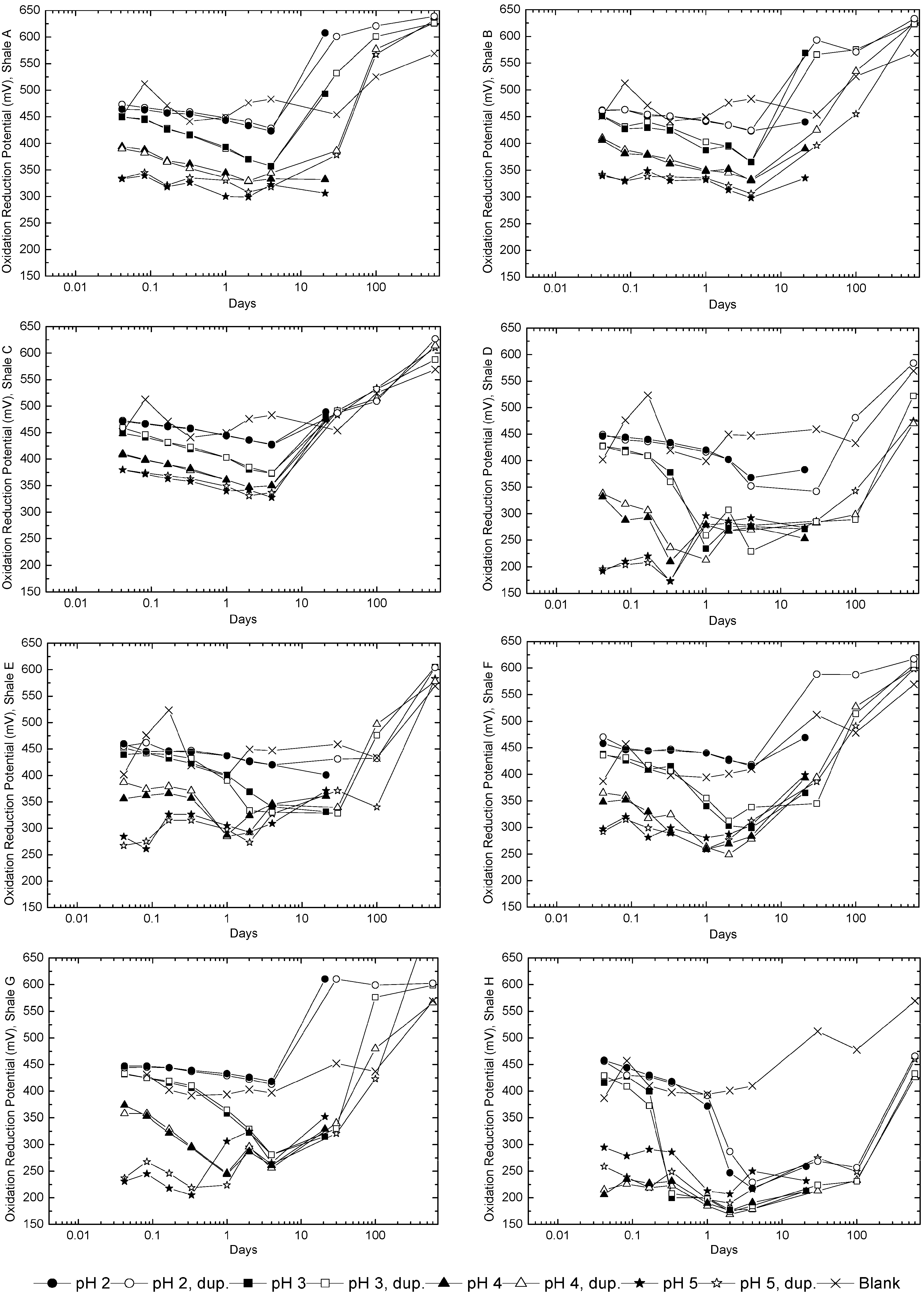
3.2. Sample Acidification and Leaching

As the experiment was not conducted in a temperature controlled chamber, solution temperatures followed ambient temperatures of 19 to 29 °C. Temperature has been shown to impact on the weathering rates of pyrite [27], however we assume this effect is negligible over the range observed here. Dissolved oxygen (DO) measurements confirmed that conditions remained oxygenated (7.4–9.4 mg/L) for all samples over the sampling period.

pH varied significantly over time and between samples over the 600 day reaction period (Figure 1). Shales A, B, C, E, F, and G experienced an overall decline in solution pH from their initial set point after 100 days. Conversely Shale D and particularly H exhibited significant increases in pH, up to the 100 day sampling time. This variation is likely due to the presence of dolomite in Shales D and H (Table 2). The buffering capacity was overcome by 600 days with all pH values reducing.

ORP results (Figure 2) tended to reflect the pH values, with lower pH solutions generally recording higher ORP values. The ORP values recorded were also consistently within the range considered to be a high oxidation potential often encountered in ARD environments, i.e., >+300 mV [13]. ORP values were relatively stable until between 4 and 21 days (except Shales D and H) and then increased up until 600 days reflecting the drop in pH (data may be found in the Supplementary Information).

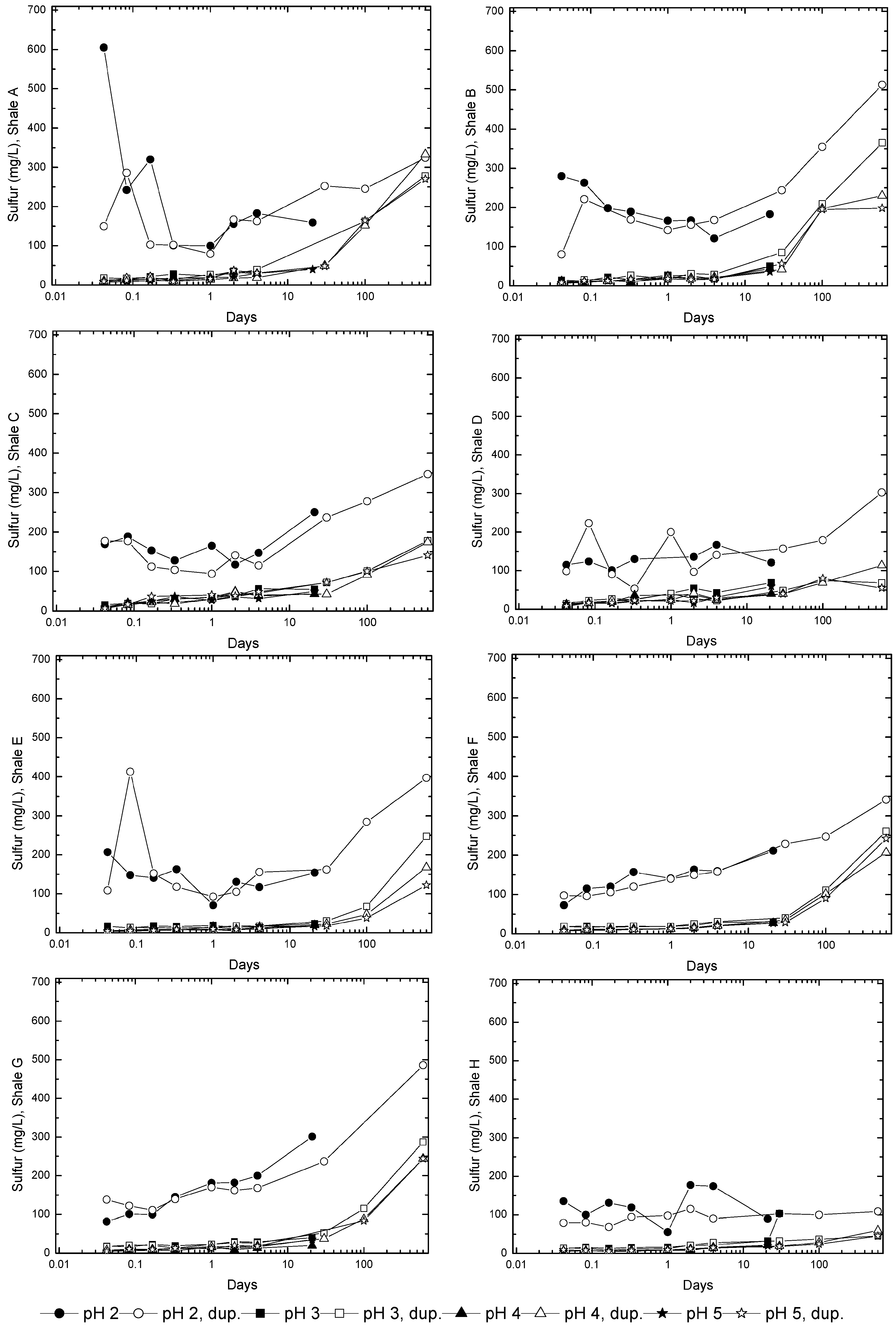
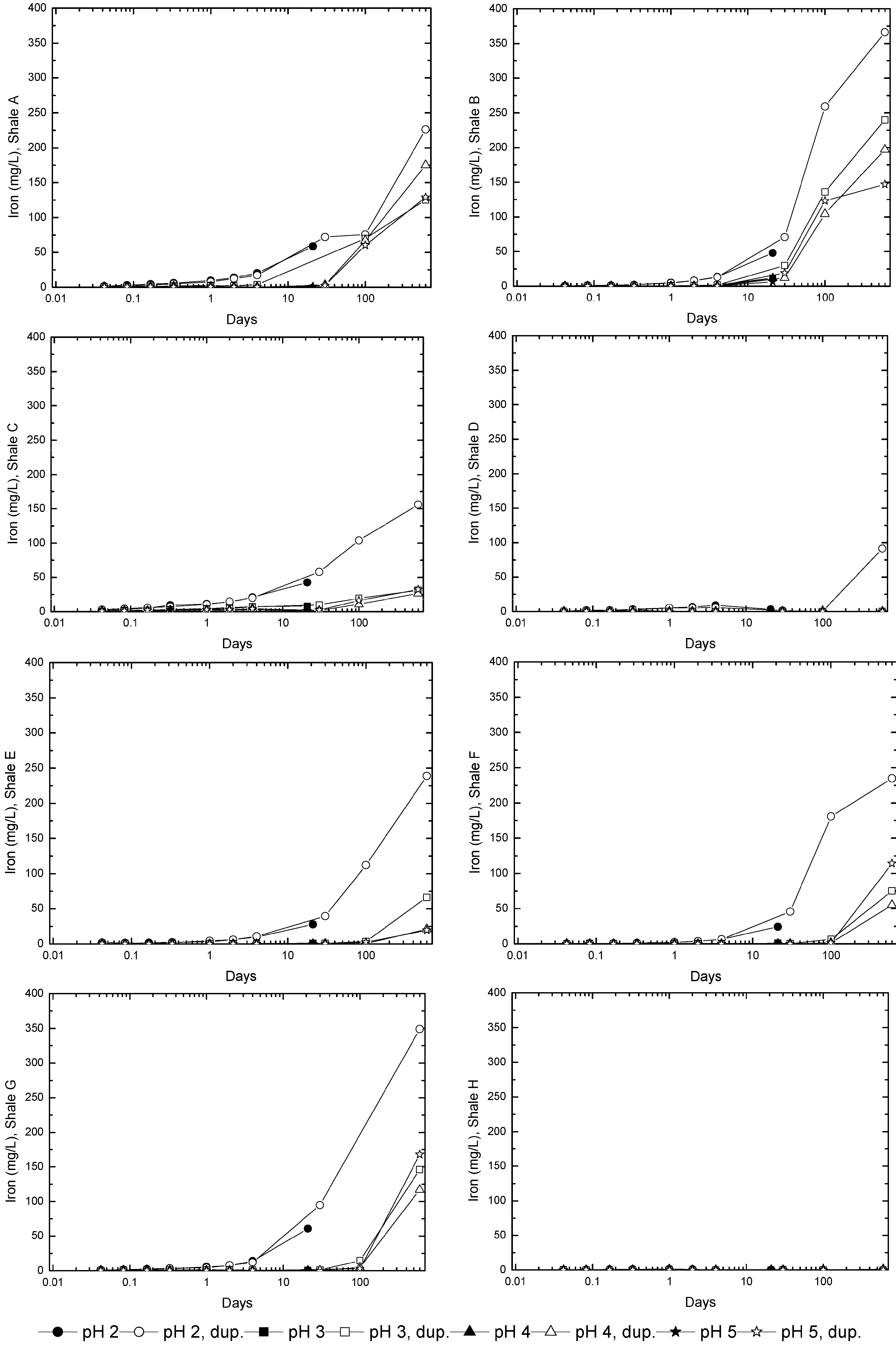
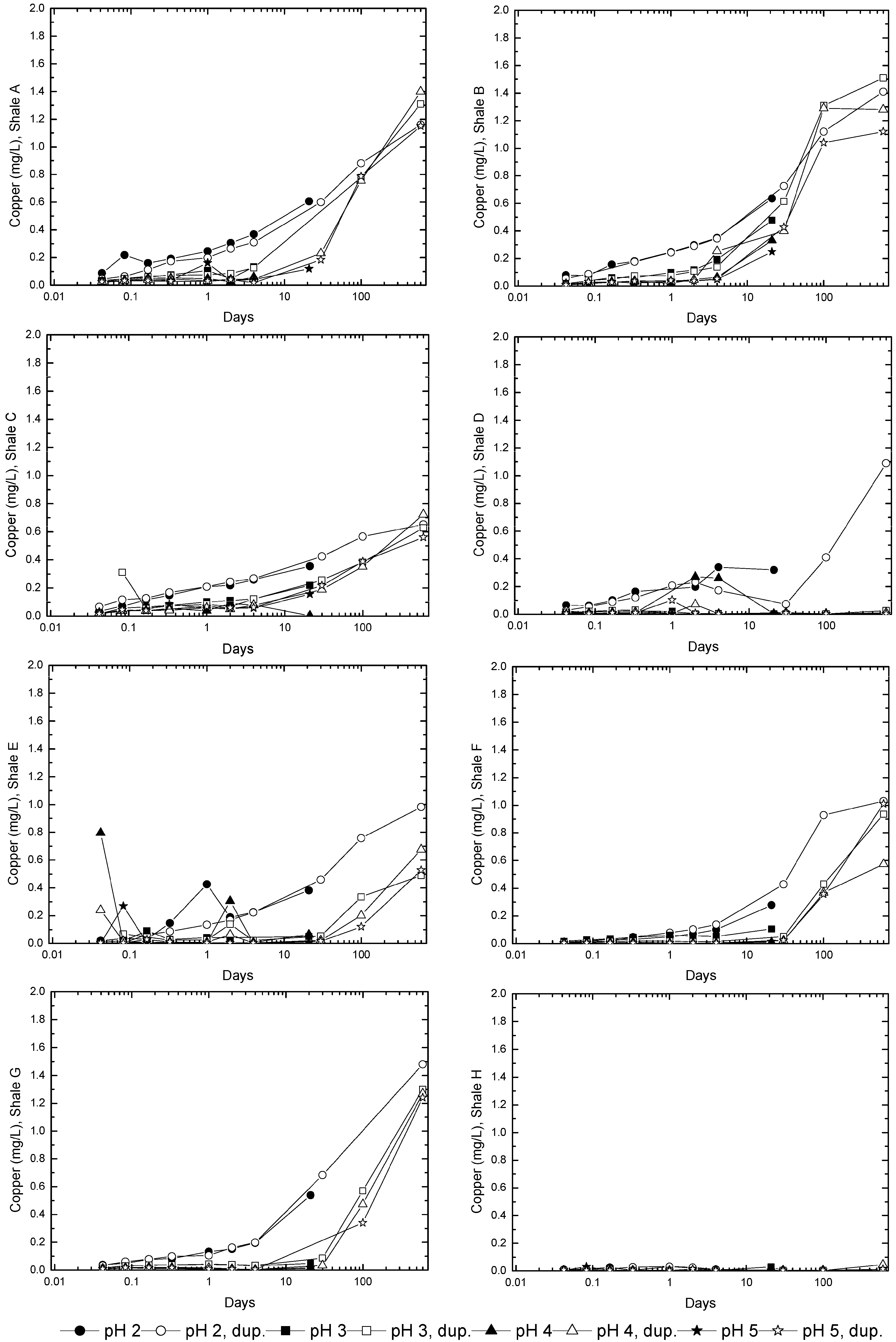
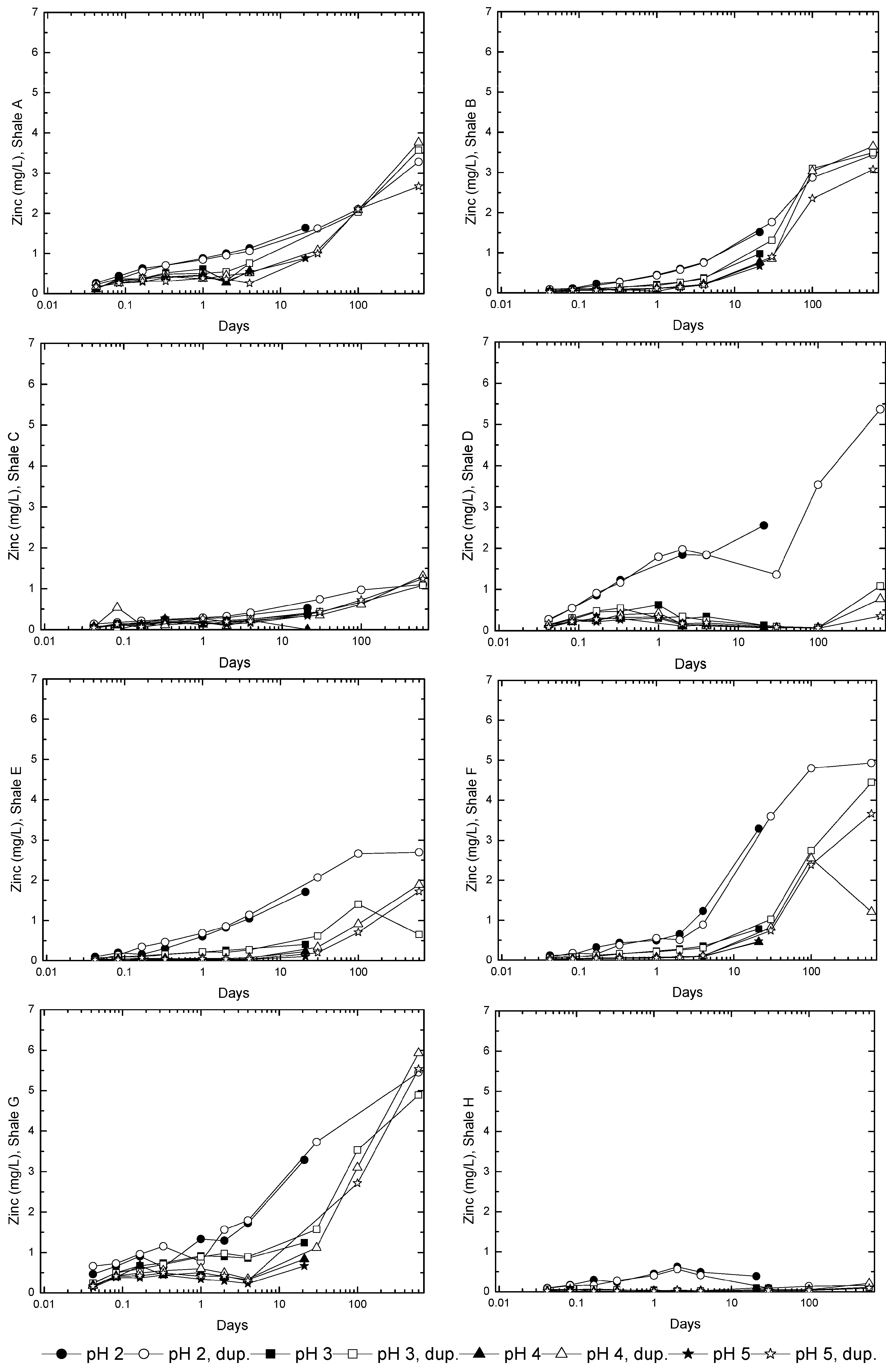
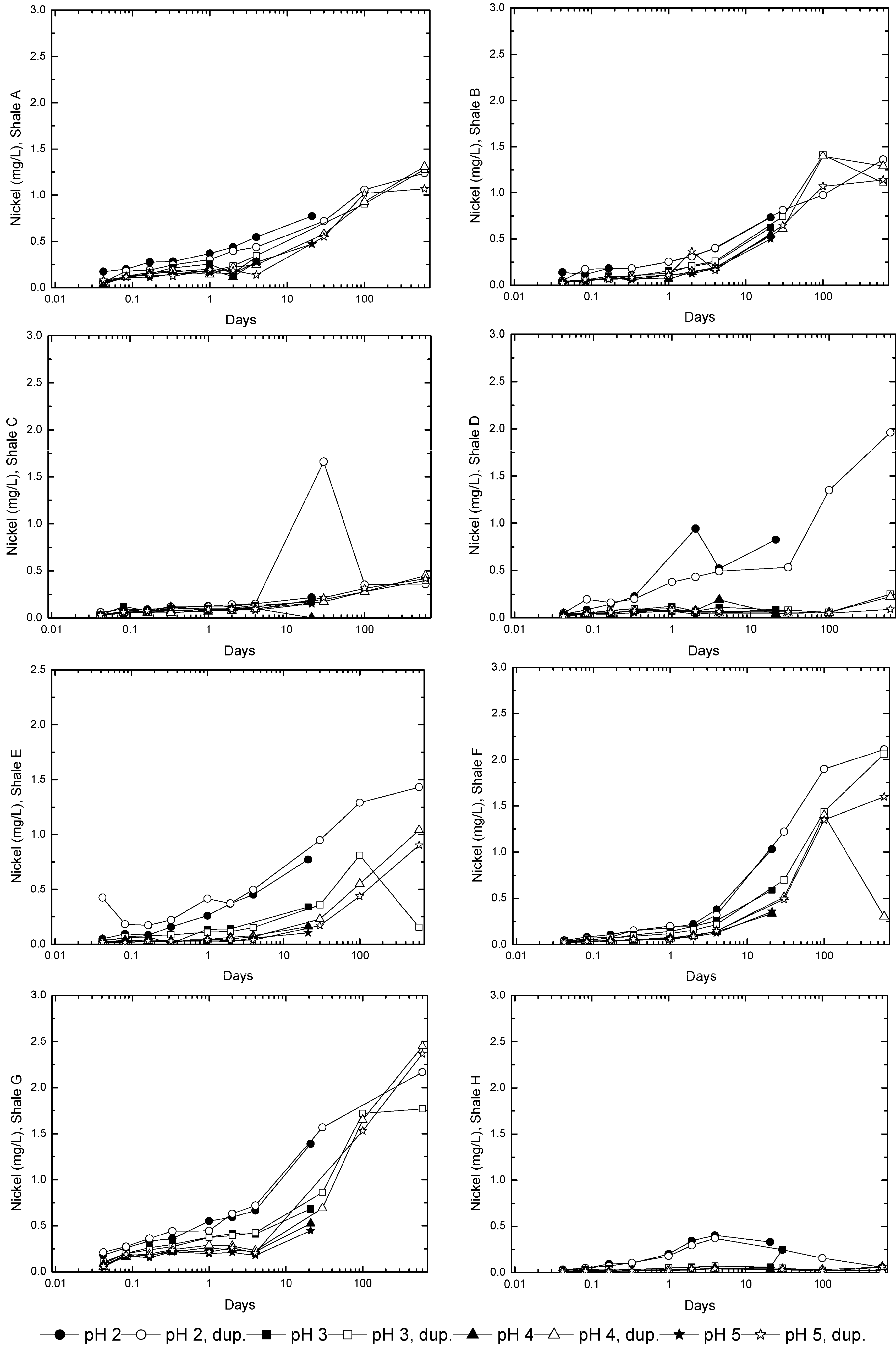
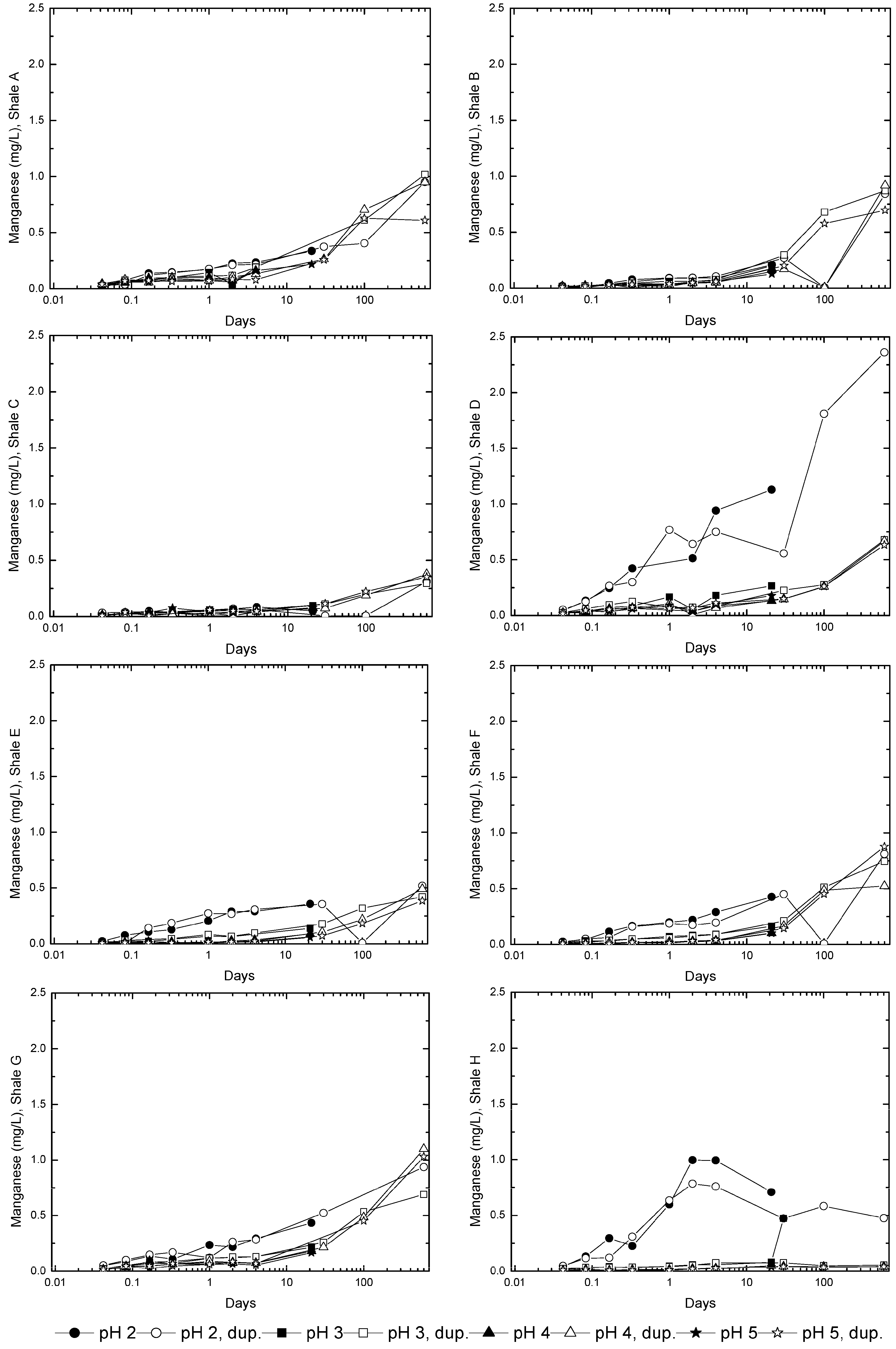
3.3. Evolution of Sulfur and Metal Concentrations

TRXRF was used to measure a spectrum of elements, however only a sub-sample of results is reported here for illustrative purposes. Results presented include S, Fe, Ni, Cu, Zn and Mn concentrations and are shown in Figure 3, Figure 4, Figure 5, Figure 6, Figure 7 and Figure 8, respectively. S in solution correlates to sulfuric acid concentrations and hence acidity. Figure 3 shows that S concentrations generally remained below 200 mg/L for all samples (except Shale A for a short period, decreasing probably due to the formation of sulfur-bearing precipitates) until approximately 10 days after the commencement of the experiment. After this time period, S concentrations increased significantly for all samples except for Shale D which increased after 100 days and H which remained generally unchanged. These concentrations correlate to the pH values observed (Figure 1) as pH values also generally dropped after 10 days. In addition Figure 3 shows there is little change to S concentrations when the initial pH is reduced from 5 to 3, but a large increase in S concentration when the pH is reduced further to 2. As noted below, the increase of S into solution over the experiment is probably due to the dissolution of metal sulfide minerals.

Leachate metal concentrations generally increased for all elements over the 600 days (Figure 4, Figure 5, Figure 6, Figure 7 and Figure 8), most significantly for Shales A, B, C, E, F and G, reflecting the increased acidity of these samples. Samples with an initial pH of 2 reported significantly higher metal concentrations in the leachate which sequentially reduced with each increase in pH value.

Figure 1. Solution pH recorded over time for all reaction vessels for all samples. Points on lines mark sample intervals from experiment commencement and 1, 2, 3, and 8 h, and 1, 2, 4, 21, 30, 100 and 600 days (logarithmic scale). The legend indicates initial sample pH.

Figure 1. Solution pH recorded over time for all reaction vessels for all samples. Points on lines mark sample intervals from experiment commencement and 1, 2, 3, and 8 h, and 1, 2, 4, 21, 30, 100 and 600 days (logarithmic scale). The legend indicates initial sample pH.

Figure 2. Oxidation reduction potential (ORP) recorded over time for all reaction vessels for all samples. Points on lines mark sample intervals from experiment commencement and 1, 2, 3, and 8 h, and 1, 2, 4, 21, 30, 100 and 600 days (logarithmic scale). The legend indicates initial sample pH.

Figure 2. Oxidation reduction potential (ORP) recorded over time for all reaction vessels for all samples. Points on lines mark sample intervals from experiment commencement and 1, 2, 3, and 8 h, and 1, 2, 4, 21, 30, 100 and 600 days (logarithmic scale). The legend indicates initial sample pH.

Figure 3. Solution Sulfur concentration recorded over time for all reaction vessels for all samples. Points on lines mark sample intervals from experiment commencement and 1, 2, 3, and 8 h, and 1, 2, 4, 21, 30, 100 and 600 days (logarithmic scale). The legend indicates initial sample pH.

Figure 3. Solution Sulfur concentration recorded over time for all reaction vessels for all samples. Points on lines mark sample intervals from experiment commencement and 1, 2, 3, and 8 h, and 1, 2, 4, 21, 30, 100 and 600 days (logarithmic scale). The legend indicates initial sample pH.

Figure 4. Solution Iron concentration recorded over time for all reaction vessels for all samples. Points on lines mark sample intervals from experiment commencement and 1, 2, 3, and 8 h, and 1, 2, 4, 21, 30, 100 and 600 days (logarithmic scale). The legend indicates initial sample pH.

Figure 4. Solution Iron concentration recorded over time for all reaction vessels for all samples. Points on lines mark sample intervals from experiment commencement and 1, 2, 3, and 8 h, and 1, 2, 4, 21, 30, 100 and 600 days (logarithmic scale). The legend indicates initial sample pH.

Figure 5. Solution Nickel concentration recorded over time for all reaction vessels for all samples. Points on lines mark sample intervals from experiment commencement and 1, 2, 3, and 8 h, and 1, 2, 4, 21, 30, 100 and 600 days (logarithmic scale). The legend indicates initial sample pH.

Figure 5. Solution Nickel concentration recorded over time for all reaction vessels for all samples. Points on lines mark sample intervals from experiment commencement and 1, 2, 3, and 8 h, and 1, 2, 4, 21, 30, 100 and 600 days (logarithmic scale). The legend indicates initial sample pH.

Figure 6. Solution Copper concentration recorded over time for all reaction vessels for all samples. Points on lines mark sample intervals from experiment commencement and 1, 2, 3, and 8 h, and 1, 2, 4, 21, 30, 100 and 600 days (logarithmic scale). The legend indicates initial sample pH.

Figure 6. Solution Copper concentration recorded over time for all reaction vessels for all samples. Points on lines mark sample intervals from experiment commencement and 1, 2, 3, and 8 h, and 1, 2, 4, 21, 30, 100 and 600 days (logarithmic scale). The legend indicates initial sample pH.

Figure 7. Solution Zinc concentration recorded over time for all reaction vessels for all samples. Points on lines mark sample intervals from experiment commencement and 1, 2, 3, and 8 h, and 1, 2, 4, 21, 30, 100 and 600 days (logarithmic scale). The legend indicates initial sample pH.

Figure 7. Solution Zinc concentration recorded over time for all reaction vessels for all samples. Points on lines mark sample intervals from experiment commencement and 1, 2, 3, and 8 h, and 1, 2, 4, 21, 30, 100 and 600 days (logarithmic scale). The legend indicates initial sample pH.

Figure 8. Solution Manganese concentration recorded over time for all reaction vessels for all samples. Points on lines mark sample intervals from experiment commencement and 1, 2, 3 and 8 h, and 1, 2, 4, 21, 30, 100 and 600 days (logarithmic scale). The legend indicates initial sample pH.

Figure 8. Solution Manganese concentration recorded over time for all reaction vessels for all samples. Points on lines mark sample intervals from experiment commencement and 1, 2, 3 and 8 h, and 1, 2, 4, 21, 30, 100 and 600 days (logarithmic scale). The legend indicates initial sample pH.

Fe concentrations in solution (Figure 4) behaved similarly to those of S, due to its association with S in the minerals pyrite and marcasite. No other major metal sulfide phases were detected in the X-ray diffractometry of the reactants, which contributed to the reasonably good relationship between S and Fe in Figure 3 and Figure 4. Concentrations of Fe increased most significantly after 10 days for all samples except for Shales D and H, with higher concentrations recorded at lower initial pH values. Ni concentrations increased over the 600 days for all samples (Figure 5) except Shale H even though this sample reported the highest Ni concentration within the raw material (Table 4). Shale C also presented low concentrations within the leachate, however this sample was also characterised by a low nickel concentration in the initial shale sample (Table 4).

Cu followed similar trends to that of sulfur and iron as Shales A, B, C, E, F and G reported increasing copper concentrations throughout the experiment correlating with the overall decline in pH and rise in ORP (Figure 6). As with many other metals Shale H recorded relatively low Cu concentrations, remaining stable at the 0–5 μg/L level. Zn concentrations also mirrored trends in pH, with all shales displaying an increase in Zn concentration except for Shale H which was only found to vary minimally over time (Figure 7) [28].

Compared with other metals reported, Mn showed higher potential to leach from Shale D and H (Figure 8). This is likely to be due to a higher initial Mn concentration in these samples combined with the less oxidising conditions in the vessel (Figure 2). Mn has previously been found to be more mobile with a move to more reducing conditions to a greater extent than other metallic elements such as Fe, Cu and Zn [2].

Pourbaix diagrams, which show the likely stable form of an element given a certain range of pH and ORP, are depicted in Figure 9 for selected metals. The charting of the pH and ORP results from this investigation show that when air is in excess, leachates from the shale can produce mildly oxidizing alkaline conditions to strongly oxidizing acidic (highly reactive) conditions depending on the mineral assemblage. In this instance there is a linear relationship between pH and ORP for the samples, with lower pH associated with increased ORP values, and progression towards this highly reactive state with increasing time.

Generally, Shale A, B, C and G fall closer to the reactive end of sample measurements, while Shale D and in particular Shale H fall closer to the less reactive end, with Shale E and F showing a wider range, but falling largely in between. The less reactive nature of Shales D and H is likely due to the presence of dolomite and halite present in these samples (Table 2). The strongly oxidizing and low pH conditions for all samples presented in the pourbaix diagrams would likely result in all sulfur being present as sulfate, and thus any precipitates probably forming oxy-hydroxysulfates.

The pourbaix diagram for Fe indicates that most of the Fe is present as Fe²⁺. However for samples at high pH conditions, i.e., greater than 5.8–6.0, which is particularly true for Shale D and H, Fe is likely present as solid Fe₂O₃. This interpretation is reiterated by the low Fe²⁺ concentrations determined for Shale D and H (Figure 3). This characteristic can also have important impacts for the concentrations of other metals in solution. Precipitation of iron oxide minerals will tend to result in the adsorption of other ions with co-precipitation and removal of these other ions from solution as a consequence. The pourbaix diagrams for Mn, Cu, Ni and Zn suggest their most likely ionic form in solution is Mn²⁺, Cu²⁺, Ni²⁺ and Zn²⁺ for the range of conditions observed in the reaction vessels. However, the metal concentration results determined and presented in Figure 4 to Figure 8 suggest for Shale D and H the metal concentrations remain lower than anticipated until the point at which Fe solubilizes, releasing the adsorbed metals into solution. This is in contrast to Shales A, B, C and G which recorded higher metal concentrations in solution throughout the experiment as the lower solution pH and iron solubilization prevented these minerals from forming.

Biofilms were not observed in the reaction vessels, and while some amount of biological activity may have been present, it was not enough to warrant further investigation. It may have been that the prevailing oxidizing conditions, coupled with the low resultant pH and low nutrient content, may have suppressed biological activity. While it possible that microbially-produced H₂S could have left the reaction vessels, this gas would have been particularly noticeable in the laboratory and was not noticed at any time.

Figure 9. Pourbaix diagrams for elements of interest. Phases are based on chemical reaction models which combine the element of interest with H₂O [29].

Figure 9. Pourbaix diagrams for elements of interest. Phases are based on chemical reaction models which combine the element of interest with H₂O [29].

4. Conclusions

This research demonstrates the importance not only of sample buffering capacity, but also dissolution and reaction kinetics on system pH and release of metal leachate from shale materials for ARD processes. pH, ORP and metal concentrations in solution changed significantly throughout the 600 day experiment, which could have significant effects on overall site impacts when occurring on a gravel pad site. Importantly, this research demonstrates the buffering capacity of minerals such as dolomite to halt metal leaching by shales for extended periods of time. However, this capacity does become exhausted over long periods, even years, resulting in a reduction in pH and an increase in metals which eventually leach into solution into groundwater and potentially surface discharge into sensitive receiving waters.

Although this investigation has demonstrated the importance of reaction kinetics on ARD processes there are experimental improvements that may be made. As reaction kinetics are important it follows that water retention times are equally important. Ideally this work would be conducted in flow-through systems on-site whereby the effects of local geology, water flow rates, soil and water chemistry, dilution by uncontaminated groundwater and local could be incorporated into the analysis.

The use of gravel platforms to elevate infrastructure above boggy muskeg areas with seasonally frozen ground overlying permafrost is common practice throughout the Arctic and sub-Arctic. This work has shown that some shale materials from these sites have the potential to be acid generating and to leach metals into the environment over time, even if the material initially contains buffering materials. The natures of the processes involved are complex and time dependant, and careful investigation is warranted to ensure suitable ARD mitigation strategies are adopted.

References

1. Neculita, C.M.; Zagury, G.J.; Bussiere, B. Passive treatment of acid mine drainage in bioreactors using sulfate-reducing bacteria: Critical review and research needs. J. Environ. Qual. 2007, 36, 1–16. [Google Scholar] [CrossRef]
2. Pareuil, P.; Penilla, S.; Ozkan, N.; Bordas, F.; Bollinger, J.C. Influence of reducing conditions on metallic elements released from various contaminated soil samples. Environ. Sci. Technol. 2008, 42, 7615–7621. [Google Scholar] [CrossRef]
3. Akcil, A.; Koldas, S. Acid Mine Drainage (AMD): Causes, treatment and case studies. J. Clean Prod. 2006, 14, 1139–1145. [Google Scholar] [CrossRef]
4. Tabak, H.H.; Scharp, R.; Burckle, J.; Kawahara, F.K.; Govind, R. Advances in biotreatment of acid mine drainage and biorecovery of metals: 1. Metal precipitation for recovery and recycle. Biodegradation 2003, 14, 423–436. [Google Scholar] [CrossRef]
5. Pandey, P.K.; Sharma, R.; Roy, M.; Pandey, M. Toxic mine drainage from Asia’s biggest copper mine at Malanjkhand, India. Environ. Geochem. Health 2007, 29, 237–248. [Google Scholar] [CrossRef]
6. Luis, A.T.; Teixeira, P.; Almeida, S.F.P.; Ector, L.; Matos, J.X.; da Silva, E.A.F. Impact of acid mine drainage (AMD) on water quality, stream sediments and periphytic diatom communities in the surrounding streams of Aljustrel mining area (Portugal). Water Air Soil Pollut. 2009, 200, 147–167. [Google Scholar] [CrossRef]
7. Askaer, L.; Schmidt, L.B.; Elberling, B.; Asmund, G.; Jonsdottir, I.S. Environmental impact on an arctic soil-plant system resulting from metals released from coal mine waste in Svalbard (78 degrees N). Water Air Soil Pollut. 2008, 195, 99–114. [Google Scholar] [CrossRef]
8. El Khalil, H.; El Hamiani, O.; Bitton, G.; Ouazzani, N.; Boularbah, A. Heavy metal contamination from mining sites in South Morocco: Monitoring metal content and toxicity of soil runoff and groundwater. Environ. Monit. Assess. 2008, 136, 147–160. [Google Scholar]
9. Khan, M.S.; Zaidi, A.; Wani, P.A.; Oves, M. Role of plant growth promoting rhizobacteria in the remediation of metal contaminated soils. Environ. Chem. Lett. 2009, 7, 1–19. [Google Scholar] [CrossRef]
10. Brake, S.S.; Dannelly, H.K.; Connors, K.A.; Hasiotis, S.T. Influence of water chemistry on the distribution of an acidophilic protozoan in an acid mine drainage system at the abandoned Green Valley coal mine, Indiana, USA. Appl. Geochem. 2001, 16, 1641–1652. [Google Scholar] [CrossRef]
11. Lee, J.S.; Chon, H.T. Hydrogeochemical characteristics of acid mine drainage in the vicinity of an abandoned mine, Daduk Creek, Korea. J. Geochem. Explor. 2006, 88, 37–40. [Google Scholar] [CrossRef]
12. Migaszewski, Z.M.; Galuszka, A.; Paslawski, P.; Starnawska, E. An influence of pyrite oxidation on generation of unique acidic pit water: A case study, podwisniowka quarry, Holy Cross Mountains (south-central Poland). Pol. J. Environ. Stud. 2007, 16, 407–421. [Google Scholar]
13. Tutu, H.; McCarthy, T.S.; Cukrowska, E. The chemical characteristics of acid mine drainage with particular reference to sources, distribution and remediation: The Witwatersrand Basin, South Africa as a case study. Appl. Geochem. 2008, 23, 3666–3684. [Google Scholar] [CrossRef]
14. Smith, R.M.; Sobek, A.A.; Arkele, T.; Sencindiver, J.C.; Freeman, J.K. Extensive Overburden Potentials for Soil and Water Quality; EPA-600/2-76-185; U.S. Environmental Protection Agency (EPA): Washington, DC, USA, 1976.
15. McDonald, D.M.; Webb, J.A.; Taylor, J. Chemical stability of acid rock drainage treatment sludge and implications for sludge management. Environ. Sci. Technol. 2006, 40, 1984–1990. [Google Scholar] [CrossRef]
16. Sapsford, D.J.; Bowell, R.J.; Dey, M.; Williams, K.P. Humidity cell tests for the prediction of acid rock drainage. Miner. Eng. 2009, 22, 25–36. [Google Scholar]
17. Ardau, C.; Blowes, D.W.; Ptacek, C.J. Comparison of laboratory testing protocols to field observations of the weathering of sulfide-bearing mine tailings. J. Geochem. Explor. 2009, 100, 182–191. [Google Scholar]
18. Carbone, C.; Dinelli, E.; Marescotti, P.; Gasparotto, G.; Lucchetti, G. The role of AMD secondary minerals in controlling environmental pollution: Indications from bulk leaching tests. J. Geochem. Explor. 2013, 132, 188–200. [Google Scholar] [CrossRef]
19. Wobrauschek, P. Total reflection X-ray fluorescence analysis—A review. X-Ray Spectrom. 2007, 36, 289–300. [Google Scholar] [CrossRef]
20. Zou, H.F.; Xu, S.K.; Fang, Z.L. Determination of chromium in environmental samples by flame AAS with flow injection on-line coprecipitation. At. Spectrosc. 1996, 17, 112–118. [Google Scholar]
21. Capota, P.; Baiulescu, G.E.; Constantin, M. The analysis of environmental samples by ICP-AES. Chem. Anal. 1996, 41, 419–427. [Google Scholar]
22. Ammann, A.A. Inductively coupled plasma mass spectrometry (ICP-MS): A versatile tool. J. Mass Spectrom. 2007, 42, 419–427. [Google Scholar] [CrossRef]
23. Townsend, A.T. The accurate determination of the first row transition metals in water, urine, plant, tissue and rock samples by sector field ICP-MS. J. Anal. At. Spectrom. 2000, 15, 307–314. [Google Scholar] [CrossRef]
24. Wang, H.; Bigham, J.A.; Tuovinen, O.H. Oxidation of marcasite and pyrite by iron-oxidizing bacteria and archaea. Hydrometallurgy 2007, 88, 127–131. [Google Scholar]
25. Gurung, S.R.; Stewart, R.B.; Gregg, P.E.H.; Bolan, N.S. An assessment of requirements of neutralising materials of partially oxidised pyritic mine waste. Aust. J. Soil Res. 2000, 38, 329–344. [Google Scholar] [CrossRef]
26. Canadian Council of Ministers of the Environment (CCME). Canadian Water Quality Guidelines for the Protection of Aquatic Life: Summary Table, Updated 7.1, December 2007; Canadian Council of Ministers of the Environment (CCME): Winnipeg, MB, Canada, 2007. Available online: https://www.halifax.ca/environment/documents/CWQG.PAL.summaryTable7.1.Dec2007.pdf (accessed on 20 January 2014).
27. Chandra, A.P.; Gerson, A.R. The mechanisms of pyrite oxidation and leaching: A fundamental perspective. Surf. Sci. Rep. 2010, 65, 293–315. [Google Scholar] [CrossRef]
28. Chuan, M.C.; Shu, G.Y.; Liu, J.C. Solubility of heavy metals in a contaminated soil: Effects of redox potential and pH. Water Air Soil Pollut. 1996, 90, 543–556. [Google Scholar] [CrossRef]
29. Takeno, N. Atlas of Eh-pH Diagrams: Intercomparison of Thermodynamic Databases; Open File Report No. 419. Geological Survey of Japan: Tsukuba, Japan, 2005. Available online: http://www.gsj.jp/GDB/openfile/files/no0419/openfile419e.pdf (accessed on 20 January 2014).