An Agent-Based Co-Evolutionary Multi-Objective Algorithm for Portfolio Optimization


AGH University of Science and Technology, Department of Computer Science, 30-059 Kraków, Poland
*
Author to whom correspondence should be addressed.
Symmetry 2017, 9(9), 168; https://doi.org/10.3390/sym9090168
Submission received: 19 June 2017
/
Revised: 8 August 2017
/
Accepted: 17 August 2017
/
Published: 23 August 2017
Abstract
:Algorithms based on the process of natural evolution are widely used to solve multi-objective optimization problems. In this paper we propose the agent-based co-evolutionary algorithm for multi-objective portfolio optimization. The proposed technique is compared experimentally to the genetic algorithm, co-evolutionary algorithm and a more classical approach—the trend-following algorithm. During the experiments historical data from the Warsaw Stock Exchange is used in order to assess the performance of the compared algorithms. Finally, we draw some conclusions from these experiments, showing the strong and weak points of all the techniques.
1. Introduction
The portfolio optimization problem is very important for every investor willing to risk their money in order to obtain potential benefits exceeding the average rate of profit of the capitalist economy. Before the 1950s, investors relied on common sense, experience or even premonitions in order to construct their portfolios. Then, some theories establishing the relation between the risk and the potential return of the investment were formulated [1]. Finally, the investors had solid tools at hand to ease the complex process of investing their money. Obviously, the proposed theories could not make each of us a millionaire—they are merely used as a yet another source of analytic information that can be taken into consideration.
In this paper we propose the agent-based co-evolutionary multi-objective algorithm for portfolio optimization and we will compare the quality of its solutions to the those obtained with the use of evolutionary, co-evolutionary and trend-following algorithms.
Two groups of experiments were carried out. In the first experiment, data from the year 2010—a year of moderate stock market rises—was used. In the second experiment, data was used from the year 2008, which was an extremely difficult time for investors—the Warsaw Stock Exchange (WSE) WIG20 index (WIG20 is the capitalization-weighted stock market index of the twenty largest companies on the Warsaw Stock Exchange) lost over 47% in value. The model of co-evolutionary multi-agent system (CoEMAS), developed in our previous papers, allows for using many different biologically and socially inspired computation and simulation techniques and algorithms within one coherent agent-based system. Such techniques can be introduced in a very natural way because of the decentralized character of the CoEMAS model. They can also be combined together on the basis of the agent-based approach, eventually causing a synergistic effect and emergent phenomena to appear during experiments.
Thanks to the possibilities of introducing the co-evolutionary interaction and sexual selection mechanisms, we have techniques for maintaining population diversity, which are very important in the case of multi-modal optimization and multi-objective optimization problems. One such mechanism, based on the co-evolution of sexes and the sexual selection, is proposed in this paper. The multi-objective portfolio optimization problem is used as a testbed for assessing the agent-based co-evolutionary multi-objective algorithm and the proposed technique for maintaining population diversity. This is of course only a small fragment of much broader research aiming at the formulation of a general model of agent-based systems for computing and simulation, utilizing biologically and socially inspired techniques and algorithms.
The rest part of the paper is organized as follows. First, we will introduce basic concepts of multi-objective optimization and agent-based evolutionary algorithms and we will present related research on applications of the bio-inspired techniques to financial and economic problems. In the next part of the paper the evolutionary algorithm, the co-evolutionary algorithm, and the proposed agent-based co-evolutionary algorithm are presented. Also, the trend-following technique used as a reference point in our experiments is described. The last part of the paper includes the results of two types of experiments, discussion of the results, and conclusions.
1.1. Multi-Objective Optimization
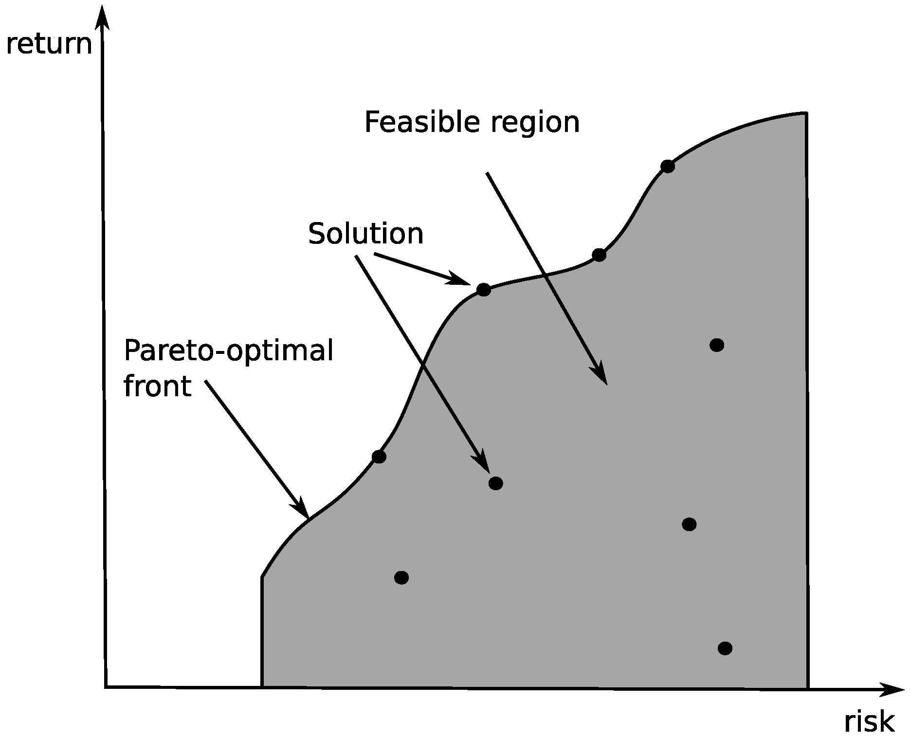
The main goal of continuous optimization is to find the very best solution from a most likely infinite set of possible solutions. The optimization procedure relies on finding and comparing feasible solutions until no better solution can be found. Each solution can be classified as a good or a bad one in terms of the specific objective we are interested in. For example, we could define an objectives in terms of costs of fabrication, efficiency of a technological process, etc. In the case of multi-objective optimization, as opposed to single-objective optimization, there is no clearly defined optimum. Instead, we have to deal with a set of trade-off optimal solutions. They are generally known as Pareto-optimal solutions [2].
The vast majority of the real-world problems involve more than one objective. That is why it is so crucial to develop methods that can efficiently solve this type of optimization problem [2,3].
The multi-objective optimization problem (MOOP) deals with more than one objective function. It turns out that the objectives are most likely contradictory, which makes the MOOP difficult to solve. In fact, it is the most common situation we will ever encounter. Following [3], the formal definition of the MOOP is as follows:
The constraints and bounds (, and are the constraint functions) constitute a decision space (set ) [3]. Any solution that satisfies all the constraints and bounds is called the feasible solution [3].
Because in the case of multi-objective problems there are many minimized/maximized criteria, we have to somehow indicate which solution is better than the other one. In order to avoid converting the minimization to maximization (or the maximization to minimization) problems, the additional operator ⊲ has to be defined—notation indicates that the solution is better than the solution for the objective (regardless of whether the criterion is minimized or maximized). Now, the dominance relation can be defined—it is said that the solution dominates the solution () if and only if [2]:
A solution is non-dominated when it is not dominated by any other solution of a given problem. A solution in the Pareto sense of the multi-objective optimization problem is a set of all non-dominated alternatives from the set . The set of all non-dominated solutions (see Figure 1) can be then presented to a human decision-maker who chooses one of them.
1.2. Evolutionary Multi-Objective Algorithms
During over 20 years of research on evolutionary algorithms (EAs) for multi-objective optimization many techniques have been proposed [4,5,6,7,8]. Deb [3] provides the typology of the evolutionary multi-objective algorithms (EMOAs). He distinguishes elitist and non-elitist techniques, although his typology includes also so-called constrained EMOAs—the techniques that support constraint handling [3]. Elitist EMOAs, among others, include Rudolph’s algorithm [9], the distance-based Pareto genetic algorithm (GA) [10], strength Pareto EA (SPEA) [11] and SPEA2 [12], the Pareto-archived evolution strategy [13], multi-objective messy GA [14] and multi-objective micro GA [15]. Non-elitist EMOAs include the vector-optimized evolution strategy [16], random weighted GA [17], weight-based GA [18], niched-pareto GA [19], non-dominated sorting GA (NSGA) [20] (in NSGA-II the elitism was added), multiple objective GA [21], and distributed sharing GA [22].
The main difference between these two groups of techniques is the utilization of the so-called elite-preserving operators. Thanks to the elite-preserving techniques the best individuals can be directly transferred to the next generation, omitting the actual selection mechanism. Of course there is a rotation within the elite set—if the algorithm finds a better solution then it replaces one of the individuals from the elite.
1.3. Maintaining Population Diversity in Evolutionary Multi-Objective Algorithms
Maintaining population diversity and introducing speciation are two very important issues in the case of evolutionary algorithms. Techniques used for obtaining these goals are called niching (or speciation) mechanisms.
Maintaining population diversity and finding many different solutions through the use of niching techniques are very important in the case of multi-modal optimization problems and of course also in the case of multi-objective optimization problems, since we are interested in finding all non-dominated solutions—the whole Pareto frontier should be evenly “covered” by the individuals.
The niching techniques allow for finding multiple solutions (forming sub-populations or species of individuals) via the modification of the mechanism of selecting individuals for a new generation (crowding model [23]), a modification of the parent selection mechanism (fitness sharing technique [24] or sexual selection mechanism [25]). Other possibilities include limited application of the selection and/or the recombination mechanisms (by explicit grouping of individuals into sub-populations [26] or by introducing the environment, in which the individuals are located and which restricts the possibilities of recombination [27,28]). Some of the above techniques were used in the multi-objective evolutionary algorithms. For example the fitness-sharing technique was used in Hajela and Lin genetic algorithms for multi-objective optimization based on weighting method [29]. Fitness sharing was also used by Fonseca and Fleming in their multi-objective genetic algorithm using a Pareto-based ranking procedure [21]. In the niched Pareto genetic algorithm (NPGA) [19] the fitness-sharing mechanism was used in the objective space during the tournament selection (when the mechanism based on the domination relation failed to choose the winner). In the case of a non-dominated sorting genetic algorithm (NSGA) [20] fitness sharing is used within each set of non-dominated individuals separately in order to maintain the population diversity. In the strength Pareto evolutionary algorithm (SPEA) [2] a special type of fitness sharing (based on the Pareto dominance) is used in order to maintain the population diversity.
Co-evolutionary techniques for evolutionary algorithms are applicable in the cases where the fitness function formulation is difficult (or even impossible), like in the problem of generating strategies for computer games. However, co-evolutionary algorithms can also be used as techniques for maintaining population diversity because they eventually lead to speciation and formation of sub-populations.
Generally speaking, co-evolutionary techniques can be classified as competitive [30] or co-operative [31]. In the case of competitive co-evolution two (or more) individuals coming from the same or different sub-populations compete in a game and their “competitive fitness functions” are calculated on the basis of their performance [32]. In the case of co-operative co-evolutionary algorithms a problem is decomposed into sub-problems solved by different sub-populations [31].
In [33] the co-evolutionary algorithm with predator–prey model and spatial graph-like structure for multi-objective optimization was proposed. Deb later modified this algorithm in such a way that predators eliminated prey on the basis of the weighted sum of all criteria [3]. Additional modification was introduced by Li [34]. In his algorithms prey could migrate within the environment. In [35] the model of cooperative co-evolution was applied to multi-objective optimization.
Sexual selection results from the fact that the proportion of individuals from each sex within a given species is almost 1:1 and the reproduction costs are much higher in the case of one of the sexes (usually females). These facts lead to female–male co-evolution, in which the females evolve to keep the reproduction at the optimal level and the males evolve to attract females. Sexual selection is considered to be one of the mechanisms responsible for biodiversity and sympatric speciation [36,37]. The sexual selection mechanism was used in the multi-objective evolutionary algorithms as a tool for maintaining the population diversity.
In [38] Allenson proposed the genetic algorithm with sexual selection for multi-objective optimization. The number of sexes was the same as the number of criteria of the given problem being solved. The sex of the child was determined randomly and the child replaced the poorest individual from its sex in the population. The partner for reproduction was selected on the basis of preferences encoded within the genotype of the given individual.
Lis and Eiben proposed the multi-sexual genetic algorithm (MSGA) for multi-objective optimization [39]. One sex for each criterion was used. The recombination operator was used randomly. The partners for reproduction were chosen from each sex separately with the use of a ranking mechanism. The offspring was created with the use of a multi-parent crossover operator. The sex of child was the same as the sex of the parent that provided most of the genes. The group of Pareto-optimal individuals found so far was maintained during the run of the algorithm.
Bonissone and Subbu [40] further developed Lis and Eiben’s algorithm. Additional mechanisms for determining the sex of the offspring were proposed. One of them was to determine the sex at random and the second mechanism was based on the solution encoded within the individual—the sex of the child was determined by the criterion for which it best fitted.
Co-evolution of species and sexual selection are the biological mechanisms responsible for sympatric speciation and the introduction of diversity of the population. However, these techniques were not widely used as mechanisms for maintaining the population diversity and as speciation mechanisms for classical evolutionary algorithms. It was probably caused by the centralized nature of these algorithms and the problems with introducing some more advanced techniques based on the ecological phenomena existing in nature. On the other hand, co-evolution and sexual selection can be quite easily introduced into agent-based evolutionary algorithms because they quite well suit the decentralized character of these algorithms. In fact in some of the previous papers we developed the niching techniques for CoEMAS working on the basis of sexual selection and co-evolution [41].
1.4. Agent-Based Co-Evolutionary Algorithms
The idea of agent-based evolutionary algorithms was proposed in [42]. In this approach the individuals are agents which “live” within an environment and act independently, making the decisions about reproduction, migration and interactions with other agents. The selection mechanism is based on resources, which are needed for performing every action, so when an agent runs out of the resources it dies and is removed from the multi-agent system. The resources are also used to maintain the functional integrity of the system [43].
The model of agent-based evolutionary algorithms was further developed in [44]. In this work the model of co-evolutionary interactions between species and sexes was introduced—basically it allowed for constructing the agent-based evolutionary algorithms utilizing many co-evolving species and sexes. Co-evolutionary multi-agent systems (CoEMAS) were applied with success to multi-modal optimization (for example see [41]) and multi-objective optimization (for example see [45,46,47]), in which case it allowed for constructing novel and very effective mechanisms for maintaining the population diversity [48]. The CoEMAS model was then generalized and the bio-inspired multi-agent system for simulation and computations was proposed in [49]. This approach was applied to the modeling and simulation of species formation processes based on the co-evolutionary interactions.
Our generalized model allows for use together the computation and simulation techniques within one coherent system. It was possible due to the agent-based approach. Using agent-based simulation algorithms together with biologically and socially inspired computation techniques opens up quite new possibilities. We can simulate biological, social, economical and political systems, additionally using the computation algorithms within agents for optimization and learning. Additionally, we can simulate selected biological mechanisms and introduce them into social and economical simulations. It is possible to observe emergent phenomena resulting from the interactions of the agents acting within the system. Using the agent-based approach, it is quite natural and relatively easy to model and simulate whole artificial societies, with different modes of production and social relations. It is possible to simulate the effects of social stratification, social power, political systems etc. Hence, our model is not just a tool for constructing computational systems but the more general approach allowing for the agent-based simulations of biological and social systems, additionally allowing for using the computational techniques within the agents. This opens quite new possibilities of introducing learning, perception and reasoning components into the social, economical and biological simulations.
In this paper we focus on only one aspect of our research—agent-based computing systems. We introduce the co-evolutionary multi-agent system with two co-evolving sexes for solving the multi-objective portfolio optimization problem, which serves as a testbed for our algorithm and techniques. We will compare the results of the proposed system with the results of genetic algorithm, co-evolutionary algorithm and trend-following approach in order to asses the quality of the results and the ability to maintain the population diversity.
2. Previous Research
The goal of the portfolio optimization is to decide in what proportions various assets should be held in order to obtain the best portfolio according to some criterion. The foundation of all modern theories for building efficient portfolios is Harry Markowitz’ modern portfolio theory (MPT) proposed in 1952 [50,51] and its extension consisting of introducing risk-free assets to the model proposed in 1958 by James Tobin [52]. These theories and models are the formal foundations of risk—rate of return investment decision-making.
In recent years there has been a growing interest in research on bio-inspired artificial intelligence algorithms for solving economic and financial problems [53,54,55,56,57]. Below, we present some selected applications of the bio-inspired techniques in the investment decision support systems.
In [58] the authors presented a genetic algorithm used for investment decision support. The main task of the algorithm was to choose (on the basis of historical data) the company to invest in. In the system some logical operations were performed on the historical data and the task of the genetic algorithm was to choose proper logical operators in the given situation.
The genetic algorithm for the automatic generation of trade models represented by financial indicators was proposed in [59]. The goal of the proposed algorithm was to select the parameters for indicators. The authors presented three algorithms: the genetic algorithm (which performed rather poorly because it converged to local minima and was weak when it came to generalization); the genetic algorithm with the fitness-sharing technique developed by X. Yin and N. Germay [60] (it generally performed better than the genetic algorithm); and the genetic algorithm with the fitness-sharing technique developed by the authors themselves (with the best capability for generalization).
The authors of [61] proposed a genetic algorithm for finding trading rules for the S&P 500 index. The genetic algorithm was used to select the structures and parameters for rules composed of functions organized into a tree and a returned value (which indicated whether the stocks should be bought or sold at a given price). The authors used the following components of the rules: functions operating on historical data, numerical or logical constants, and logical functions (used to build more complex rules).
In [62], genetic programming was used to predict bankruptcy. The authors used historical data to build a function assessing whether the particular company was heading toward financial problems. Approximately 75% of the test data was classified correctly.
Evolutionary algorithms were also used to design and optimize the artificial neural networks designated to automate trading (trading is a process of buying and selling financial instruments). An example of such a system was described in [63]—the authors pointed out that the trading rules were unsophisticated but the systematic execution of them could lead to some substantial returns.
Very interesting modifications to the standard evolutionary approach—quantum-inspired EAs—were used for option pricing model calibration in [64].
The evolutionary approach was compared with some simple investing strategies and the stock market index in [65]. In some cases the proposed technique outperformed the basic version of the buy and hold strategy as well as the market index.
The authors of [66] extended the classical mean-variance optimization problem with a third objective—robustness. As a result, it was possible to group the sets of portfolios according to their reliability and provide this additional information to a human decision-maker.
In [67] the authors used multi-objective genetic algorithm for portfolio optimization. Two objectives based on the Markowitz model were used: the risk and the rate of return. The authors of [68] used three higher moment models: mean-variance-skewness with three objectives, mean-variance-skewness-kurtosis with four objectives, and mean-variance-skewness-kurtosis with eight objectives. Three median models with two objectives were used: the median value at risk, median conditional value at risk, and median mean absolute deviation. They constructed multi-objective problems using these models and used the NSGA-II multi-objective evolutionary algorithm to solve them. The real financial data coming from Egyptian Exchange (EGX) was used during the experiments. Generally speaking, the authors concluded that the median models outperformed the higher moments models during the experiments with real data coming from the emerging market.
The co-evolutionary multi-agent system using predator–prey interactions was presented in [69]. The system was run against well-known test problems as well as portfolio optimization problem. The results obtained from both groups of experiments proved that the CoEMAS approach is a robust technique, providing more general solutions that can be used in many different market conditions.
The agent-based co-evolutionary genetic programming approach was also applied with success to investment strategy generation [70,71]. During the experiments the agent-based approach was compared to the evolutionary algorithm, a co-evolutionary algorithm, and the buy-and-hold strategy. Also in this case the results of experiments confirmed that the agent-based approach led to obtaining more general investment strategies.
The co-evolutionary multi-agent system with sexual selection was applied to multi-objective optimization problems in [72]. This was the very first attempt to realize agent-based sexual selection in the co-evolutionary system for multi-objective optimization. There were two sexes used but they were not connected with any particular objectives of the problem being solved. The partner for reproduction was chosen on the basis of the level of resources. This algorithm was compared experimentally with SPEA and NSGA multi-objective evolutionary algorithms. The results showed that agent-based approach maintains the population diversity much better than the “classic” algorithms.
In [73] another variant of the agent-based sexual selection was proposed. In this algorithm each agent used vector of weights in order to choose the partner for reproduction. This algorithm was compared experimentally with SPEA2 and NSGA-II multi-objective evolutionary algorithms. It was found that each step of the “classical” algorithms is computationally much more complex than the single step of the agent-based approach.
In this paper we propose the agent-based multi-objective co-evolutionary algorithm, which is applied to portfolio optimization and compared to evolutionary and co-evolutionary algorithms. The main contributions of this paper, as compared to the works presented above, are as follows:
- The idea, design and realization of the agent-based multi-objective co-evolutionary algorithm for portfolio optimization. As compared to our previous research, we propose here different architectures, algorithms and a modified technique for maintaining population diversity. The proposed algorithm utilizes two co-evolving sexes and the competition for limited resources mechanism (dominating agents obtain resources from the dominated ones) in order to obtain high quality solutions and maintain population diversity. The number of the sexes corresponds with the number of objectives of the problem being solved. Each sub-population (sex) is optimized with the use of different objectives. The agents choose partners for the reproduction from the opposite sex and the decision is made on the basis of the quality of the solutions and also on the basis of the resources possessed by the agents.
- Design (including the adjustments needed for solving the multi-objective portfolio optimization problem) and realization of a genetic algorithm and co-evolutionary algorithm (including the fitness function, all genetic operators and the diversity maintaining mechanisms) for multi-objective portfolio optimization.
- Experimental comparison of evolutionary, co-evolutionary, proposed agent-based co-evolutionary and trend-following algorithms with the use of historical data dating two years prior (2010 and 2008) with quite different stock market trends.
The research presented in this paper is the part of our more general research project aiming at the development of a model, architectures, and algorithms for biologically and socially inspired agent-based systems for use in simulation and computation. Our approach would unify many different biologically and socially inspired techniques on the basis of the agent-based approach. The agent-based approach provides a common architecture for designing and implementing mechanisms and algorithms inspired by biological and social mechanisms in a very natural way similar to reality-based techniques.
3. Evolutionary, Co-Evolutionary and Agent-Based Algorithms for Portfolio Optimization
All of the algorithms mentioned in this chapter are implemented to calculate the best possible portfolio throughout a specified time period, which forces an adjustment to the changing market’s conditions and provides a trading strategy whereby we can follow the portfolio’s composition adjustments made on a daily basis.
3.1. Genetic Algorithm
Genetic algorithms (GAs) [74] are well-known and popular techniques of dealing with multi-objective optimization problems (MOOPs) [3].
Every time we try to use GA to solve a given problem we have to adjust it accordingly. In our implementation each potential solution should be encoded inside a chromosome. Each chromosome represents the portfolio composition (it is a normalized vector of double values representing the percentage share of each stock)—the same representation is used in the co-evolutionary and the agent-based co-evolutionary algorithms. Before the first round of computation, the entire population is created from scratch using random values in chromosomes.
The following modified GA operations have been implemented:
- mutation—the mutation operator changes exactly one value, , representing the percentage share of a specific stock i (each time the value i is chosen randomly) to ( (0,1) is chosen randomly). After that, we have to normalize the vector. Mutation_coefficient determines which part of the population will be subjected to the mutation operator.
- selection—the breeding_coefficient determines which part of the population will be subjected to crossover operator. Selection is based on the fitness function (only the fittest part of the population will be selected);
- crossover—after selecting chromosomes eligible for the reproduction, each pair of chromosomes is subjected to crossover operator. As a result, new chromosomes are created (each pair produces two new chromosomes) and added to the population. Crossover chooses left and right points (both are chosen randomly) which cut parents’ chromosomes in the way presented in the Figure 2a. Children are created according to the process shown in the Figure 2b.
Apart from that, an extinction mechanism has been implemented. At the end of each GA round the part of the population that has the lowest fitness is exterminated. The extinction_coefficient determines which part of the population will be subjected to extinction.
3.1.1. Pseudo-code
The pseudo-code of the GA is presented in Algorithm 1. We start by evaluating each chromosome using the fitness function (described in Section 3.1.2), which uses current stock prices. The fittest individuals are allowed to reproduce (this is further controlled by the breeding_coefficient that determines which part of the population will be subjected to crossover operator). New individuals are merged with the existing population. After that, the mutation is applied to a part of the least fit population to assure that population is diverse (in fact it is a way of implementing a reinitialization method, mentioned in [2]) and we do not miss any potentially better solutions. Then, we destroy some of the least fit individuals—in such a way we can control the overall population size and we get rid of the individuals with chromosomes not likely to be successful in the future. Finally, we return the best individual, which becomes our trading strategy for the next day (we adjust our current portfolio to the fittest individual solution).
| Algorithm 1: GA pseudo-code |
 |
3.1.2. Fitness Function
Fitness is calculated according to the following formula (for portfolio with N stocks):
where:
- is the value of the portfolio’s fitness calculated for specific ;
- is the percentage share of a specific stock i in the whole portfolio;
- returns the price of the stock i for the specific .
Clearly, the fitness function favors portfolios which have the highest day-to-day increase in value. Of course ,such methods of calculating fitness have many drawbacks, e.g., they completely omits the aspect of risk associated with the investing in highly volatile stocks. However, it turns out that in spite of this obvious flaw the algorithm performs quite well.
3.2. Co-Evolutionary System
Contrary to the genetic algorithm described in Section 3.1, in the co-evolutionary algorithm (CEA) two sub-populations coexist side by side. Each individual represents a potential solution to the portfolio optimization problem. The risk-oriented sub-population tries to optimize the risk (the lower risk value the better), whereas the return oriented sub-population tries to maximize expected return. Usually the greater the expected return, the riskier the investment, so our solutions will involve some trade-offs. However that should not startle us, as we have already predicted in Section 1.1 that optimization under such circumstances is not an easy task.
As presented in Figure 3, the reproduction is allowed only between the members of different sub-populations. Not every member of a particular sub-population is allowed to reproduce—only the fittest ones (fitness of a particular individual depends on the sub-population it belongs to—the fittest one in one sub-population would probably be considered as one of the weakest in another one). Thanks to this approach, the offspring that are created are very diverse. In fact, it is an application of restricted mating [2]. Some of the weakest members of both sub-populations are subjected to extinction. Because of that, we do not end up with a too-large population full of useless solutions. In the place of extinct members, the offspring of the fittest individuals are introduced to both sub-populations.
Apart from that, some members of the sub-populations are subjected to mutations in order to even further maintain the sub-population diversity. The migration mechanism has the same purpose—it is applied in order to avoid local optima. It is also described in [2] as an isolation by distance. The individuals for migration are selected at random with probability of 0.1. During the migration, selected individuals are moved from one sub-population to another—this introduces new chromosomes into the given sub-population and makes it more diverse.
The risk as well as the expected return are calculated according to capital asset pricing model (described in [75]).
3.2.1. Maintaining Population Diversity
To sum up, several mechanisms have been implemented to keep both sub-populations diverse:
- crossover is allowed only between the fittest chromosomes from different sub-populations;
- mutations introduce random genetic change;
- migration allows chromosomes to travel to different nodes.
3.2.2. Pseudo-Code
Contrary to the GA, we are dealing with two sub-populations (with different objectives) at once (see Algorithm 2). Apart from that, the pseudo-code looks very similar. The reproduction is only allowed between individuals from different sub-populations. To even further assure that populations remain diverse, we mutate part of the least fit individuals. Migration of the individuals between the nodes also helps maintaining the population diversity. Extinction helps to control population size and get rid of useless individuals. A non-dominated solution (in Pareto sense) is returned as a result.
| Algorithm 2: Co-evolutionary algorithm (CEA) pseudo-code |
 |
3.3. The Co-Evolutionary Multi-Agent System
The co-evolutionary multi-agent system (CoEMAS) is the most sophisticated system that has been implemented. CoEMAS model [44] is the result of merging co-evolutionary computations and multi-agent systems paradigms.
Such systems need an environment as well as a set of autonomous agents interacting with each other. A potential solution to the portfolio optimization problem is stored inside each agent—it is encoded within its genotype. In the CoEMAS model the environment is usually a graph with vertices (nodes) connected with the edges. Agents live within the environment, and can migrate from one node to another (looking for better living conditions), reproduce, and interact with each other. The agents need resources for every activity and these resources can be obtained from the environment or from other agents. An agent dies when it runs out of resources. Each agent can reproduce when it has enough resources—it usually selects a partner for reproduction and when it succeeds offspring are created with the use of the recombination and mutation operators.
Contrary to the co-evolutionary system described in Section 3.2 there are no sub-populations. Instead, we introduced individuals of two different sexes (see Figure 4). Each sex focuses on a different task:
- sex1—tries to achieve the lowest risk possible;
- sex2—tries to achieve the highest expected return possible.
The risk as well as the expected return is calculated due to the capital asset pricing model (defined in [75]).
3.3.1. CoEMAS Model
A formal model of the co-evolutionary multi-agent system was proposed for the first time in [44] and was further developed and generalized in [49]. Below, we will use the CoEMAS model for describing in a more formal way the co-evolutionary multi-agent system used for multi-objective portfolio optimization.
The multi-agent system with two co-evolving sexes is defined as follows:
where:
- is the set of environment types in the time t;
- is the set of environments of the in the time t;
- is the set of types of elements that can exist within the system in time t;
- is the set of vertice types that can exist within the system in time t;
- is the set of object (not an object in the sense of object-oriented programming but an object as an element of the simulation model) types that may exist within the system in time t;
- is the set of agent types that may exist within the system in time t;
- is the set of resource types that exist in the system in time t; the amount of resource of type will be denoted by ;
- is the set of information types that exist in the system, the information of type will be denoted by ;
- is the set of relations between sets of agents, objects, and vertices;
- is the set of attributes of agents, objects, and vertices; and
- is the set of actions that can be performed by agents, objects, and vertices.
The set of actions is defined as follows:
The actions have the following meaning:
- death—if the amount of the resource that an agent possesses is lower than the threshold value, the agent dies;
- mig—the agent is allowed to migrate but the probability of this action is low;
- rep—the agents from different sexes are allowed to reproduce provided that they both exceed the minimum amount of resource allowing to reproduce;
- give/get—the agent can get a resource from other, dominated agents;
- rec—agents produce offspring by means of recombination;
- mut—a mutation introduces random change to the potential solution, and normalization of the solution vector is then required;
- seek—agents appropriate to the rep as well as get operations can be found thanks to this action.
Environment type is defined in the following way:
is the set of environment types that may be connected with the environment. is the set of vertice types that may exist within the environment of type . is the set of resource types that may exist within the environment of type . is the set of information types that may exist within the environment of type .
Environment of type is defined as follows:
where is directed graph , with the function defined is the set of vertices, and is the set of arches. The distance between two nodes is defined as the length of the shortest path between them in graph . is the set of environments of types from connected with the environment (in our case it is an empty set).
Vertice type is defined in the following way:
where:
- is the set of attributes of the vertice at the beginning of its existence;
- is the set of actions which the vertice can perform at the beginning of its existence, when asked for it;
- is the set of resource types which can exist within the vertice at the beginning of its existence;
- is the set of information types which can exist within the vertice at the beginning of its existence;
- is the set of types of vertices that can be connected with the vertice at the beginning of its existence;
- is the set of types of objects that can be located within the vertice at the beginning of its existence; and
- is the set of types of agents that can be located within the vertice at the beginning of its existence.
The element of the structure of the system’s environment (vertice) of type is given by:
where:
- is the set of attributes of vertice —it can change during its lifetime;
- is the set of actions, which vertice can perform when asked for it—it can change during its lifetime;
- is the set of resources of types from that exist within the ;
- is the set of information of types from that exists within the — is the information about agents of sex1 that are located within the given vertice and is the information about the agents of sex2;
- is the set of vertices of types from connected with the vertice —in our case it is the set of four vertices (see Figure 4);
- is the set of objects of types from that are located in the vertice ;
- is the set of agents of types from that are located within the vertice .
There are two types of agents (sexes) in the system: and . The agent type is defined in the following way:
where:
- is the set of goals of the agent at the beginning of its existence;
- is the set of attributes of the agent at the beginning of its existence;
- is the set of actions which the agent can perform at the beginning of its existence;
- is the set of resource types which can be used by the agent at the beginning of its existence;
- is the set of information types which can be used by the agent at the beginning of its existence;
- is the set of types of objects that can be located within the agent at the beginning of its existence; and
- is the set of types of agents that can be located within the agent at the beginning of its existence.
is the goal get resource—an agent can get the resources from a dominated agent that is located within the same vertice, is the goal reproduce, and is the goal migrate to the other vertice.
The agent type is defined in the same way as agent—the only difference between these two types of agents is that tries to achieve the lowest risk possible and tries to achieve the highest expected return possible.
Agent (of type ) is defined in the following way:
where:
- is the set of goals, which agent tries to realize—it can change during its lifetime;
- is the set of attributes of agent —it can change during its lifetime;
- is the set of actions which agent can perform in order to realize its goals—it can change during its lifetime;
- is the set of resources of types from , which are used by agent ;
- is the set of information of types from which agent can possess and use—an agent uses information about the other agents located within the same vertice;
- is the set of objects of types from that are located within the agent ;
- is the set of agents of types from that are located within the agent .
Notation means “the set of goals of agent of type ”. is the amount of resource of type that is possessed by the agent .
Agent (of type ) is defined in the same way as agent of type .
The set of relations is defined as follows:
The first relation is defined as follows:
is the set of agents capable of performing actions seek, get. is the set of agents capable of performing the action give. This relation represents competition for resources between agents—dominated agents have to give some of its resources to dominating agents.
The second relation is defined as follows:
is the set of agents of type capable of performing actions seek, rep, rec, mut. is the set of agents of type capable of performing action rep, rec, mut. is the set of agents of type capable of performing actions seek, rep, rec, mut. is the set of agents of type capable of performing action rep, rec, mut.
This relation represents searching for reproduction partners and the process of reproduction. It can be initiated by any agent that has enough resources. Reproducing partners come from the opposite sex.
The interactions between the agents are implemented in the following way:
- co-evolution is implemented as a sequence of turns;
- in each turn every agent performs its action (the action to perform at any particular turn is chosen with a well defined probability, e.g., there is a 10% chance that the agent will try to find a partner for reproduction, and a 60% chance that the agent will try to obtain some resources from the dominated agent);
- after every agent performes some action the turn ends and the entire population of agents is checked as to whether some of them should die (when not enough resources are left after other agents take resource from them).
Each agent performs one of the above actions with some probability.
3.3.2. Pseudocode
The pseudocode of CoEMAS is presented in Algorithm 3. The actions are performed with the following probabilities:
- —with probability 0.6;
- —with probability 0.2;
- —with probability 0.1;
- —with probability 0.1.
| Algorithm 3: CoEMAS pseudocode |
 |
Similarly to Section 3.2, the mutation is used as a mean of maintaining the population diversity.
The role of the environment composed of the computation nodes is to additionally help maintain population diversity. When the agents are located within different nodes, each sub-population evolves in a different direction, so the whole population can avoid local optima (it is the model of speciation caused by the geographic separation of sub-populations). The agent can migrate between the computation nodes when the level of the resource possessed is above the minimal level (the migration costs some amount of the resource). The agent tries to migrate because it can not find asuitable partner for reproduction within the current node or it can not find dominated agents to get resources from them. The decision of migration is made with the probability 0.1.
4. Trend Following
The concept of price as the trading cue lays the foundations for trend following (TF). Contrary to the other trading strategies based on fundamental analysis (which use the factors like overall state of the economy, interest rates, production, etc. to predict the stock price), TF uses only price as the key trading variable.
Trend following basically does not try to predict when the trend will occur. Instead of that, trend followers will react to the market’s movement and adapt accordingly (an example of how TF works in practice is shown in Figure 5). This strategy simply analyses the stock prices and decides whether the current situation is suitable for buying or selling a specific stock. Market breakouts are a great buying opportunities, on the other hand when you recognize that you are wrong you exit immediately in order to cut losses. A set of predefined rules decides whether to take any action (they should recognize when the trend starts as well as when to exit) so the entire process can be easily automated. Such rules are quite simple but disciplined execution of them could lead to achieving spectacular returns year after year. It is all about cutting the losses and letting the profits run. Many leading hedge funds successfully use strategies based on trend following to manage their portfolios [76].
Another advantage of this investing method is the fact that the investor does not have to know much about what is being traded (it could be stocks, oil, gold, etc.) Normally, people tend to gather some information about the company they are willing to invest in. They analyze its market situation, competitors, financial performance, etc. which is time consuming, especially for someone who is not a professional trader. With trend following we just have to focus on elaborating trading rules that should reflect our trading strategy. After that, we can automate the decision-making process by designing and implementing our own trading system.
4.1. Types of Trends
There are three main types of trends:
- Short-term trend: any price movement that occurs over a few hours or days.
- Intermediate-term trend: general movement in price data that lasts from three weeks to six months.
- Long-term trend: any price movement that occurs over a significant period of time, often over one year or several years.
4.2. Designing Trading System Based on Trend Following
Following [76], the core of each trading system based on a trend-following strategy is a set of rules governing each buy/sell decision. More specifically, we have to devise the rules to answer the following questions:
- how much money are we willing to put on a single trade;
- when to exit (what kind of losses are acceptable);
- when to enter (when the trend has started);
- which markets are we interested in and how to split the money between them (we would like to have a diverse portfolio: stocks, gold, etc.).
These rules should reflect our investing style.
The simple moving sverage (SMA) is especially useful for highlighting the longer-term trends in a set of data points [76].
SMA is formulated as the unweighted mean of the previous N data points [76]:
where is the value of data on day j. In this case, data points will represent closing stock prices.
Entry points:
- Simple moving average (SMA) of the last N days is greater than SMA of last M days ();
- Current stock price is maximal of the last N days (that is usually a good indicator of lucrative opportunity on the market).
As soon as at least one of the above conditions is satisfied we go long (we buy a particular asset).
Exit points:
- Losses on a single trade are greater than 2% (this rule is used to quickly abandon an investment where we were wrong about its trend direction; the amount of tolerable loss solely depends on our strategy and does not have to be exactly 2%);
- The simple moving average (SMA) of the last N days is lesser than the SMA of last M days ().
As soon as the exit condition is satisfied we go short (we sell a particular asset).
Obviously the above rules are very simple and quite straightforward. Nonetheless, the system based on them proves to be robust, as shown in Section 5.
By manipulating the value of N we can seek out different types of trends, as mentioned in Section 4.1.
4.3. Pseudo-Code
The Algorithm 4 shows pseudo-code of the trend-following approach. It uses the following functions:
- SMA(i,N) calculates the simple moving average for stock i, N last days are taken into account;
- go_short(i) sell stock i;
- go_long(i) buy stock i;
- get_current_stock_price(i, day) returns stock i price for specific ;
- get_most_recent_trade_price(i) returns the price we paid for stock i (we have stock i in our portfolio);
- max(i,N) returns the maximum price for stock i in the last N days;
- N, M, maximal_value_loss modifiable parameters.
The trend-following algorithm has been implemented as a standalone R script—it is not the part of our multi-agent system.
| Algorithm 4: The trend-following pseudo-code |
 |
5. Experimental Results
In this section selected results from the experiments with data coming from the Warsaw Stock Exchange (WSE) are presented. The goal was to test the proposed and reference algorithms during different periods of time on the real data and to compare the obtained results. In the first set of experiments we used the data from the year 2010—a year of moderate stock market rises. In the second set of experiments we used the data from the year 2008—a year which was extremely hard for investors (the WIG20 lost over 47% in value). In this section we will try to answer the question as to which of the used algorithms gives the best results and under what conditions.
5.1. First Set of Tests
The first set of tests uses historical data from the year 2010 (data of three different stocks have been used). In spite of the short periods of downturns, 2010 was a year of stock market rises on the Warsaw Stock Exchange (WSE). The upward trend started in the first quarter of 2009 was maintained. The annual change of the stock exchange index (WIG) was +20.5%. The WIG reached its highest value in two years on 15 December 2010 (47,892.91 points). The minimal value of WIG in 2010 was 37,038.90 points.
Portfolio contained three assets (they are one of the biggest companies present on WSE):
- KGHM Polska Miedź S.A. (KGHM)—mining sector company;
- Telekomunikacja Polska (TPSA)—telecommunication sector company;
- PKO Bank Polski (PKOBP)—finance and insurance sector company.
The multi-agent platform has been used to run algorithms. It was configured in the following way:
- using a simulation of the trading strategy throughout the entire year 2010;
- all investing decisions have been based solely on the results from the implemented algorithms;
- the migration mechanism between computing nodes has been enabled;
- two computing nodes (with the appropriate algorithms) have been used to obtain results.
The trend-following algorithm has been tested without a multi-agent running platform as it is a standalone R script. Apart from that, it is a completely deterministic algorithm so each time we run it, we will get the same results.
5.1.1. Trend Following
5.1.1.1. Short-Term Trend Results
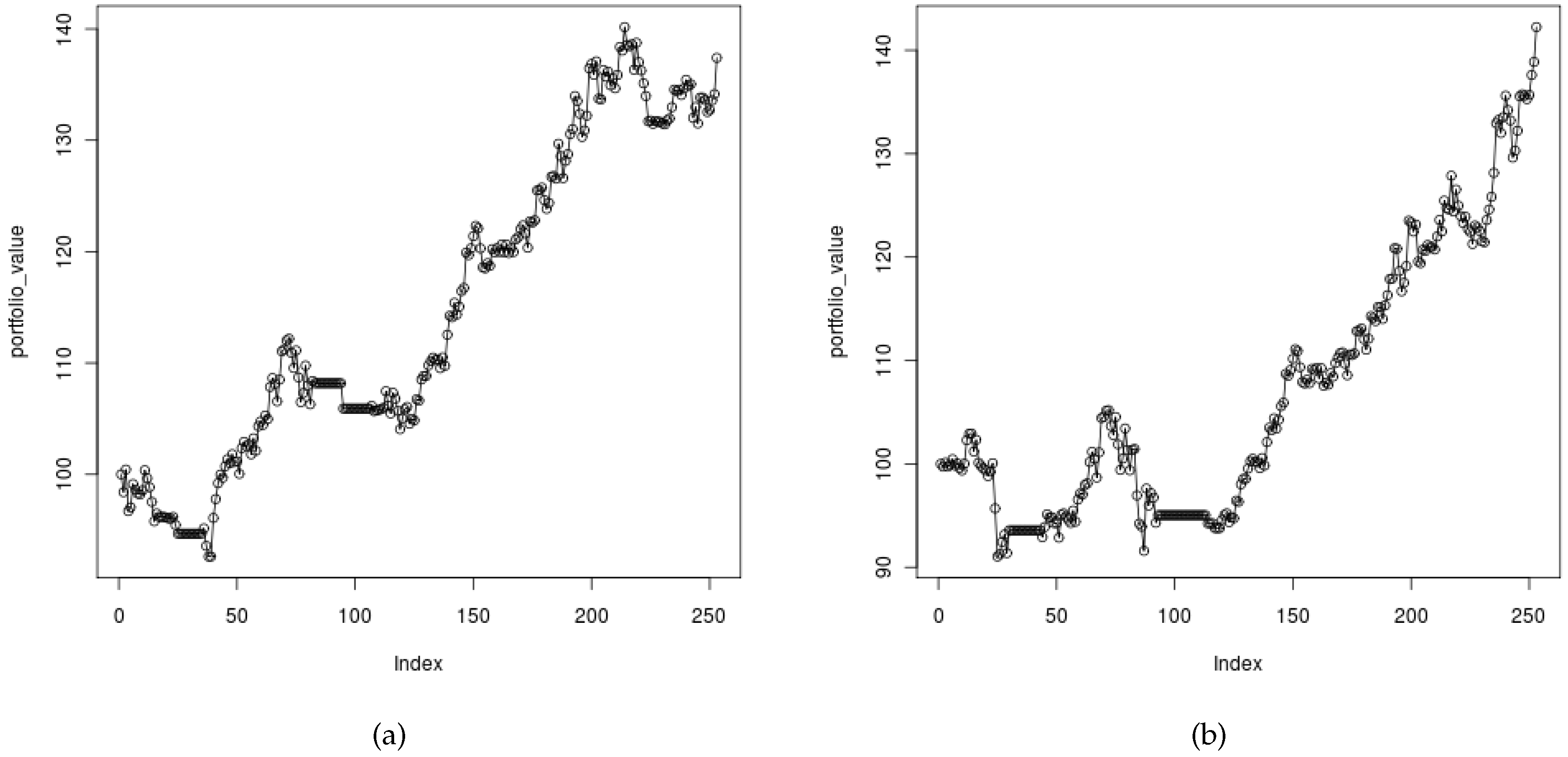
As described in Section 4, we can adjust our trading rules to seek out the short-term trends (by changing the values of N and M in the Simple Moving Average method). With values , the SMA method focused on the short-term trends.
There are easily visible periods of time (Figure 6a) when the portfolio value is not changing. It is a time when our portfolio does not contain any assets (but we still have the money). After a while, the conditions change and the trend-following algorithm decides some assets should be bought.
5.1.1.2. Intermediate-Term Trend Results
In this particular test (with values: , ), the trend-following algorithm has been adjusted to focus on the intermediate-term trends. The results are presented in Figure 6b. It can be seen that they are slightly better compared with the short-term trends approach.
It turned out that focusing on the short-term or intermediate-term trends leads to almost the same results. The intermediate-term trend approach offers a slightly better return from investment. In both cases we encountered periods of time when the portfolio contained no assets because the situation on the market was not good enough to invest in any of the available stocks.
5.1.2. Genetic Algorithm
The best results that we were able to obtain with the use of genetic algorithm are presented in Figure 7a. Apart from that, the average values of 5 runs are shown in Figure 7b. As can be easily spotted, the algorithm performs reasonably well on the average.
The following configuration was used:
- reproduction_coeff was set to 0.2;
- population size was 512;
- mutation_coeff was set to 0.1;
- extinction_coeff was set to 0.3.
5.1.3. Co-Evolutionary Algorithm
Results for the CEA, presented in Figure 8, clearly show that the return of our investment is much higher than any other algorithm could achieve. The analysis of Figure 9 explains why the results are so good—the risk associated with our portfolio is substantially higher compared to other methods. In this case the algorithm was tuned to prefer the non-dominated solutions from the return-oriented sub-population—this explains why the results provide so much return and risk.
The following configuration was used:
- reproduction_coeff was set to 0.2;
- sub-population size in each computing node was set to 64;
- number of computing nodes was set to 2;
- mutation_coeff was set to 0.1;
- extinction_coeff was set to 0.3.
5.1.4. CoEMAS
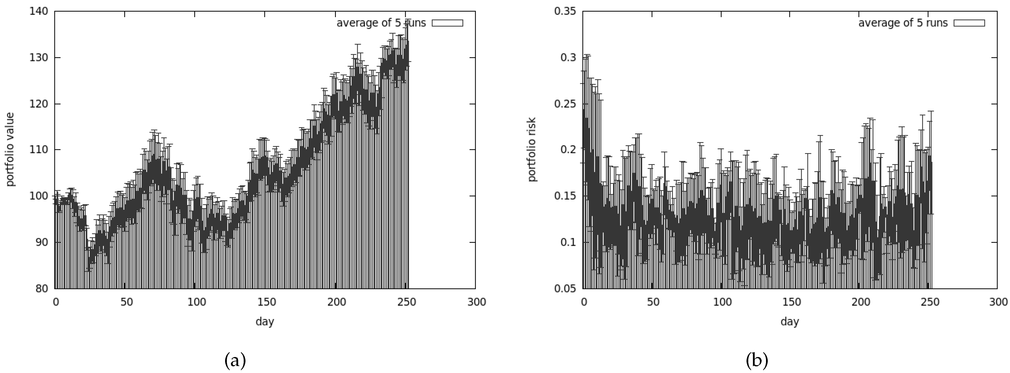
Figure 10a presents the average portfolio value in time while Figure 10b presents the average risk associated with our investments. Returns are not as spectacular as in CEA but on the other hand the amount of risk we have to take is much lower.
The following configuration was used:
- reproduction_coeff was set to 0.2;
- each sex was represented initially by 64 agents (in each computing node);
- number of computing nodes was set to 2;
- mutation_coeff was set to 0.1;
- extinction_coeff was set to 0.3.
5.1.5. Conclusions from the First Set of Tests
The first set of tests showed that all algorithms give reasonable results. It is very hard to pinpoint one approach that is substantially better than the others. The co-evolutionary system (cf. Section 3.2) outperformed other algorithms in the terms of return. Such good results can be explained by the fact that the trading strategy proposed by this algorithm is much riskier than using CoEMAS.
On the other hand, CoEMAS offers a substantially lower return but it is much safer. As Figure 10b shows, the risky moves are mixed with safe ones, resulting in a much more balanced strategy.
Trend following and the genetic algorithm can not give us any information about the risk we are taking by investing according to the results they provide. On the other hand, we can specify the rules (in the trend-following approach) that should reflect our attitude to risk-taking (cf. Section 4). With the genetic algorithm (GA) we have no such option as our abilities to customize GA are quite limited. Obviously we could test different values of coefficients responsible for simulating the evolution process but it turns out that the fitness function that does not take risk into the account is the most serious limitation.
5.2. Second Set of Tests
The second set of tests uses historical data from year 2008. The same three companies stocks as in the previous set of tests have been selected to construct our portfolio. The year 2008 was extremely hard for investors due to the crisis caused by the credit crunch back in 2007. During 2008, the WIG20 lost over 47% in value. Hence, it is tempting to run tests under such difficult circumstances in order to assess each algorithm’s ability to minimize the losses. The best solutions obtained as well as the average ones are included.
5.2.1. Trend Following
TF algorithm using the short-term trend is configured in the same way as in Section 5.1.1.1. The results are presented in Figure 11a.
TF algorithm using the intermediate-term trend is configured in the same manner as in Section 5.1.1.2. The results are presented in Figure 11b.
The intermediate-term trend seeking tends to give much better results than focusing on the short-term trends. We managed to minimize the losses thanks to the fact that we completely ceased trading during the worst time on the market.
5.2.2. Genetic Algorithm
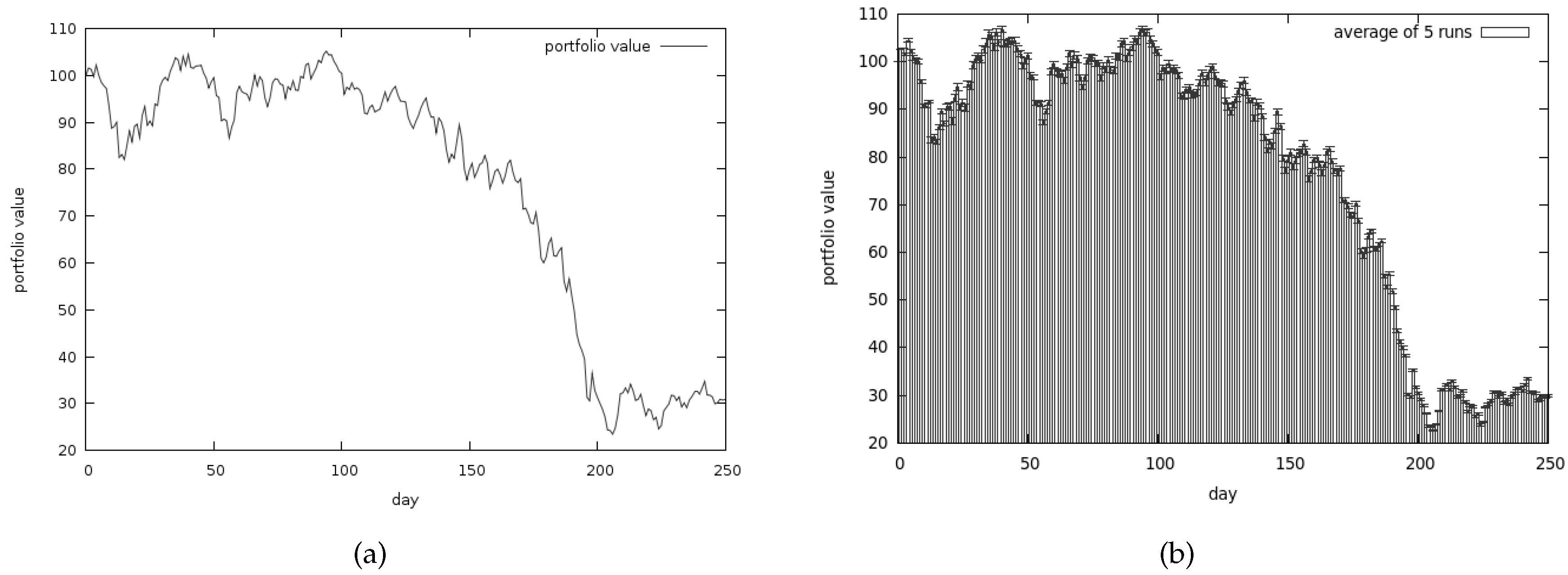
The best results that we were able to obtain are presented in Figure 12a. Apart from that, the average values of 5 runs are shown in Figure 12b. As can be easily spotted the algorithms perform reasonably well on the average (especially compared with CEA).
The following configuration was used:
- reproduction_coeff was set to 0.2;
- population size was 512;
- mutation_coeff was set to 0.1;
- extinction_coeff was set to 0.3.
5.2.3. Co-Evolutionary Algorithm
The results presented in Figure 13a are very poor (and yet they are the best results obtained from a series of tests). The average results are shown in Figure 13b.
We have lost almost all our money—approximately 70% of it. Average risk associated with our portfolio is presented in Figure 15a. As we can observe the best obtained results are quite similar to the average ones.
The following configuration was used:
- was set to 0.2;
- sub-population size in each computing node was set to 64;
- number of computing nodes was set to 2;
- was set to 0.1;
- was set to 0.3.
5.2.4. CoEMAS
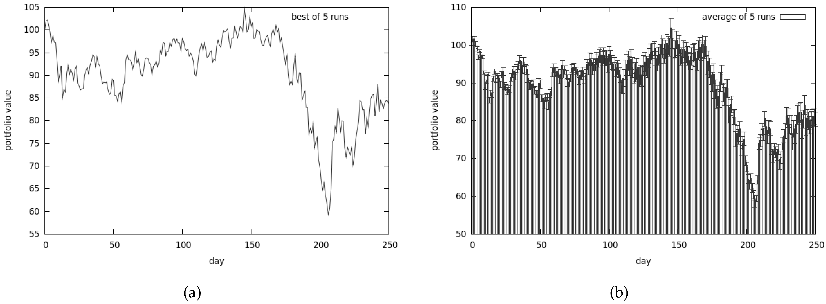
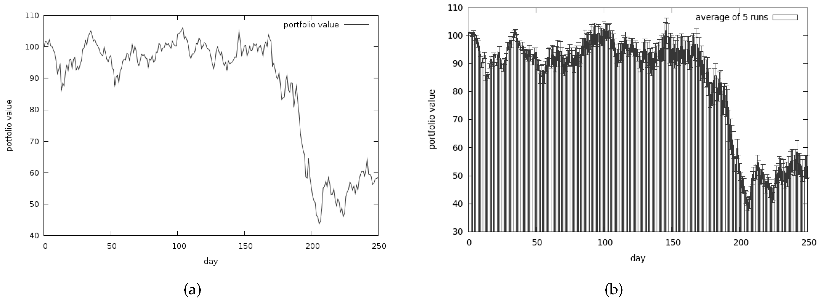
Figure 14a presents the best returns that we managed to obtain with the use of CoEMAS, while Figure 14b presents the average return. The average risk associated with our investments is shown in the Figure 15b. Once again it turns out that the average values are pretty similar to the best we managed to get. It turns out that CoEMAS performs much better in the difficult times than CEA.
The following configuration was used:
- was set to 0.2;
- each sex was represented initially by 64 agents (in each computing node);
- number of computing nodes was set to 2;
- was set to 0.1;
- was set to 0.3.
5.2.5. Conclusions from the Second Set of Tests
Clearly, the trend-following approach managed to save almost the entire capital. Losses that we had to experience due to this algorithm seem almost negligible compared with the other methods.
In spite of the fact that fitness function used in the genetic algorithm completely ignores the risk associated with the assets in portfolio, it actually performed better then the solution taking risk into consideration.
The results of the co-evolutionary algorithm are particularly poor. Almost 70% of initial money is lost. CoEMAS performs slightly better, but it is still worse than the simple genetic algorithm approach.
In summary, it appears that algorithms performing exceptionally well in a bull market can potentially lead to catastrophic losses during difficult times. The trend following algorithm has one major advantage among all discussed methods—it allows us to withdraw all our money during the periods of time that are not investor-friendly.
6. Conclusions
In this paper we have proposed the agent-based co-evolutionary multi-objective algorithm and we have applied it to the portfolio optimization problem. We have also described the proposed algorithm with the use of formal model of co-evolutionary multi-agent system (CoEMAS) proposed in our previous works. Also, the evolutionary algorithm and the co-evolutionary algorithm were implemented within our framework in order to compare the results obtained during the experiments carried out with the use of real world data coming from Warsaw Stock Exchange. Additionally, the trend-following algorithm was implemented as a standalone R script and used during the experiments as the reference point.
All implemented algorithms have been exhaustively tested using the historical data reflecting two completely different situations on the market. Taking into consideration both good and bad times leads to the conclusions that all approaches have advantages as well as disadvantages. That raises a question as to which algorithm to use if we want to build our own portfolio.
The trend-following algorithm obtains good results for unstable times because it somehow guarantees that the losses would be minimized according to our preferences. However, during stock market rise it is outperformed by other algorithms.
The proposed agent-based multi-objective co-evolutionary algorithm gives quite good results. It maintains a high level of population diversity and proposes sustainable strategies, where the risky and safe moves are mixed together. Maintaining high level of the population diversity is especially important in the times when there are rapid and frequent changes on the market. The proposed algorithm can easily adapt to the changing conditions of the environment and escape from local optima. High population diversity also leads to more robust strategies, that can be applied with success in many different conditions and situations.
Future work will include the application of our agent-based co-evolutionary approach in business intelligence systems. It would be used not only as an investment strategies generation algorithm but also as a data mining algorithm (with the use of neural and fuzzy classifiers) for market segmentation and preparation of customized products/services and targeted adds. Also, we will integrate the proposed algorithm within a framework (“virtual laboratory”) for reproducible research on artificial intelligence techniques supporting financial and economical decision-making.
Acknowledgments
This research was partially financed by AGH University of Science and Technology Statutory Fund.
Author Contributions
Rafal Drezewski proposed and developed the idea, the model, the architecture and the algorithms of the agent-based co-evolutionary approach; Rafal Drezewski co-authored the plan of experiments; Rafal Drezewski co-authored all sections of this paper; Krzysztof Doroz implemented the agent-based co-evolutionary algorithm, adapted and implemented the genetic algorithm, the co-evolutionary algorithm and implemented the trend-following algorithm; Krzysztof Doroz co-authored the plan of experiments and carried out the experiments; Krzysztof Doroz co-authored all sections of this paper.
Conflicts of Interest
The authors declare no conflict of interest. The founding sponsors had no role in the design of the study; in the collection, analyses, or interpretation of data; in the writing of the manuscript, and in the decision to publish the results.
References
- Rom, B.M.; Ferguson, K.W. Post-Modern Portfolio Theory Comes of Age. J. Investig. 1994, 3, 11–17. [Google Scholar] [CrossRef]
- Zitzler, E. Evolutionary Algorithms for Multiobjective Optimization: Methods and Applications. Ph.D. Thesis, ETH Zurich, Zürich, Switzerland, 1999. [Google Scholar]
- Deb, K. Multi-Objective Optimization Using Evolutionary Algorithms; John Wiley & Sons, Inc.: New York, NY, USA, 2001. [Google Scholar]
- Coello Coello, C.A.; Van Veldhuizen, D.A.; Lamont, G.B. Evolutionary Algorithms for Solving Multi-Objective Problems; Kluwer Academic Publishers: Dordrecht, The Netherlands, 2002. [Google Scholar]
- Osyczka, A. Evolutionary Algorithms for Single and Multicriteria Design Optimization; Physica Verlag: Heidelberg, Germany, 2002. [Google Scholar]
- Tan, K.C.; Khor, E.F.; Lee, T.H. Multiobjective Evolutionary Algorithms and Applications; Springer: London, UK, 2005. [Google Scholar]
- Villalobos, M.A. Analisis de Heuristicas de Optimizacion para Problemas Multiobjetivo. Ph.D. Thesis, Centro de Investigacion y de Estudios Avanzados del Instituto Politecnico Nacional, Mexico City, Mexico, 2005. [Google Scholar]
- Toscano, G. On the Use of Self-Adaptation and Elitism for Multiobjective Particle Swarm Optimization. Ph.D. Thesis, Centro de Investigacion y de Estudios Avanzados del Instituto Politecnico Nacional, Mexico City, Mexico, 2005. [Google Scholar]
- Rudolph, G. Evolutionary Search under Partially Ordered Finite Sets. In Proceedings of the International NAISO Congress on Information Science Innovations (ISI 2001), Dubai, UAE, 17–21 March 2001; Sebaaly, M.F., Ed.; ICSC Academic Press: Dubai, UAE, 2001; pp. 818–822. [Google Scholar]
- Osyczka, A.; Kundu, S. A new method to solve generalized multicriteria optimization problems using the simple genetic algorithm. Struct. Multidiscip. Optim. 1995, 10, 94–99. [Google Scholar] [CrossRef]
- Zitzler, E.; Thiele, L. An Evolutionary Algorithm for Multiobjective Optimization: The Strength Pareto Approach; Technical Report 43; Swiss Federal Institute of Technology: Zurich, Switzerland, 1998. [Google Scholar]
- Zitzler, E.; Laumanns, M.; Thiele, L. SPEA2: Improving the Strength Pareto Evolutionary Algorithm; Technical Report 103; Swiss Federal Institute of Technology: Zurich, Switzerland, 2001. [Google Scholar]
- Knowles, J.; Corne, D. Approximating the Nondominated Front Using the Pareto Archived Evolution Strategy. Evol. Comput. 2000, 8, 149–172. [Google Scholar] [CrossRef] [PubMed]
- Van Veldhuizen, D.A. Multiobjective Evolutionary Algorithms: Classifications, Analyses and New Innovations. Ph.D. Thesis, Graduate School of Engineering of the Air Force Institute of Technology Air University, Dayton, OH, USA, 1999. [Google Scholar]
- Coello Coello, C.; Toscano, G. Multiobjective Structural Optimization using a Micro-Genetic Algorithm. Struct. Multidiscip. Optim. 2005, 30, 388–403. [Google Scholar] [CrossRef]
- Kursawe, F. A Variant of Evolution Strategies for Vector Optimization. In Parallel Problem Solving from Nature; 1st Workshop, PPSN I; Schwefel, H., Manner, R., Eds.; Springer: Berlin, Germany, 1991; Volume 496, pp. 193–197. [Google Scholar]
- Murata, T.; Ishibuchi, H. MOGA: Multi-objective genetic algorithms. In Proceedings of the IEEE International Conference on Evolutionary Computation, Perth, Australia, 29 November–1 December 1995; IEEE Service Center: Piscataway, NJ, USA, 1995; Volume 1, pp. 289–294. [Google Scholar]
- Hajela, P.; Lee, E.; Lin, C. Genetic algorithms in structural topology optimization. In Topology Design of Structures; Bendsøe, M.P., Soares, C.A.M., Eds.; Springer: Amsterdam, The Netherlands, 1993; Volume 1, pp. 117–133. [Google Scholar]
- Horn, J.; Nafpliotis, N.; Goldberg, D.E. A Niched Pareto Genetic Algorithm for Multiobjective Optimization. In Proceedings of the First IEEE Conference on Evolutionary Computation, IEEE World Congress on Computational Intelligence, Orlando, FL, USA, 27–29 June 1994; IEEE Service Center: Piscataway, NJ, USA, 1994; Volume 1, pp. 82–87. [Google Scholar]
- Srinivas, N.; Deb, K. Multiobjective Optimization Using Nondominated Sorting in Genetic Algorithms. Evol. Comput. 1994, 2, 221–248. [Google Scholar] [CrossRef]
- Fonseca, C.; Fleming, P. Genetic Algorithms for Multiobjective Optimization: Formulation, Discussion and Generalization. In Proceedings of the Fifth International Conference on Genetic Algorithms, Urbana-Champaign, IL, USA, 17–21 July 1993; Morgan Kaufmann Publishers Inc.: San Francisco, CA, USA, 1993; pp. 416–423. [Google Scholar]
- Hiroyasu, T.; Miki, M.; Watanabe, S. Distributed Genetic Algorithms with a New Sharing Approach. In Proceedings of the Conference on Evolutionary Computation, Washington, DC, USA, 6–9 July 1999; IEEE Service Center: Piscataway, NJ, USA, 1999; Volume 1. [Google Scholar]
- Mahfoud, S.W. Crowding and preselection revisited. In Parallel Problem Solving from Nature—PPSN-II; IlliGAL Report No. 92004; Männer, R., Manderick, B., Eds.; Elsevier: Amsterdam, The Netherlands, 1992; pp. 27–36. [Google Scholar]
- Goldberg, D.E.; Richardson, J. Genetic algorithms with sharing for multimodal function optimization. In Proceedings of the 2nd International Conference on Genetic Algorithms, Cambridge, MA, USA, 29–31 July 1987; Grefenstette, J.J., Ed.; Lawrence Erlbaum Associates: Hillsdale, NJ, USA, 1987; pp. 41–49. [Google Scholar]
- Ratford, M.; Tuson, A.L.; Thompson, H. An Investigation of Sexual Selection as a Mechanism for Obtaining Multiple Distinct Solutions; Technical Report 879; Department of Artificial Intelligence, University of Edinburgh: Edinburgh, UK, 1997. [Google Scholar]
- Jelasity, M.; Dombi, J. GAS, a concept of modeling species in genetic algorithms. Artif. Intell. 1998, 99, 1–19. [Google Scholar] [CrossRef]
- Adamidis, P. Parallel Evolutionary Algorithms: A Review. In Proceedings of the 4th Hellenic-European Conference on Computer Mathematics and Its Applications (HERCMA 1998), Athens, Greece, 24–26 September 1998. [Google Scholar]
- Cantú-Paz, E. A Survey of Parallel Genetic Algorithms. Calc. Paralleles Reseaux Syst. Repartis 1998, 10, 141–171. [Google Scholar]
- Hajela, P.; Lin, C. Genetic search strategies in multicriterion optimal design. Struct. Optim. 1992, 4, 99–107. [Google Scholar] [CrossRef]
- Paredis, J. Coevolutionary Computation. Artif. Life 1995, 2, 355–375. [Google Scholar] [CrossRef] [PubMed]
- Potter, M.A.; De Jong, K.A. Cooperative Coevolution: An Architecture for Evolving Coadapted Subcomponents. Evol. Comput. 2000, 8, 1–29. [Google Scholar] [CrossRef] [PubMed]
- Darwen, P.J.; Yao, X. On evolving robust strategies for iterated prisoner’s dilemma. In Process in Evolutionary Computation; AI’93 and AI’94 Workshops on Evolutionary Computation, Selected Papers; Yao, X., Ed.; Springer: Berlin/Heidelberg, Germany, 1995; Volume 956. [Google Scholar]
- Laumanns, M.; Rudolph, G.; Schwefel, H.P. A Spatial Predator-Prey Approach to Multi-objective Optimization: A Preliminary Study. In Parallel Problem Solving from Nature—PPSN V; Eiben, A.E., Bäck, T., Schoenauer, M., Schwefel, H.P., Eds.; Springer: Berlin/Heidelberg, Germany, 1998; Volume 1498. [Google Scholar]
- Li, X. A Real-Coded Predator-Prey Genetic Algorithm for Multiobjective Optimization. In Evolutionary Multi-Criterion Optimization, Proceedings of the Second International Conference (EMO 2003), Faro, Portugal, 8–11 April 2003; Fonseca, C.M., Fleming, P.J., Zitzler, E., Deb, K., Thiele, L., Eds.; Springer: Berlin/Heidelberg, Germany, 2003; Volume 2632. [Google Scholar]
- Iorio, A.; Li, X. A Cooperative Coevolutionary Multiobjective Algorithm Using Non-dominated Sorting. In Genetic and Evolutionary Computation—GECCO 2004; Deb, K., Poli, R., Banzhaf, W., Beyer, H.G., Burke, E.K., Darwen, P.J., Dasgupta, D., Floreano, D., Foster, J.A., Harman, M., Eds.; Springer: Berlin/Heidelberg, Germany, 2004; Volume 3102–3103, pp. 537–548. [Google Scholar]
- Todd, P.M.; Miller, G.F. Biodiversity through sexual selection. In Artificial Life V: Proceedings of the Fifth International Workshop on the Synthesis and Simulation of Living Systems; Bradford Books; Langton, C.G., Shimohara, K., Eds.; The MIT Press: Cambridge, MA, USA, 1997; pp. 289–299. [Google Scholar]
- Gavrilets, S. Models of speciation: What have we learned in 40 years? Evolution 2003, 57, 2197–2215. [Google Scholar] [CrossRef] [PubMed]
- Allenson, R. Genetic Algorithms with Gender for Multi-Function Optimisation; Technical Report EPCC-SS92-01; Edinburgh Parallel Computing Centre: Edinburgh, UK, 1992. [Google Scholar]
- Lis, J.; Eiben, A.E. A Multi-Sexual Genetic Algorithm for Multiobjective Optimization. Proceedings of 1997 IEEE International Conference on Evolutionary Computation (ICEC'97), Indianapolis, IN, USA, 13–16 April 1997; IEEE Press: Piscataway, NJ, USA, 1997; pp. 59–64. [Google Scholar]
- Bonissone, S.; Subbu, R. Exploring the Pareto Frontier Using Multi-Sexual Evolutionary Algorithms: An Application to a Flexible Manufacturing Problem; Technical Report 2003GRC083; GE Global Research: Schenectady County, NY, USA, 2003. [Google Scholar]
- Dreżewski, R. Co-Evolutionary Multi-Agent System with Speciation and Resource Sharing Mechanisms. Comput. Inform. 2006, 25, 305–331. [Google Scholar]
- Cetnarowicz, K.; Kisiel-Dorohinicki, M.; Nawarecki, E. The application of Evolution Process in Multi-Agent World to the Prediction System. In Proceedings of the 2nd International Conference on Multi-Agent Systems (ICMAS 1996), Kyoto, Japan, 9–13 December 1996; Tokoro, M., Ed.; AAAI Press: Menlo Park, CA, USA, 1996; pp. 26–32. [Google Scholar]
- Cetnarowicz, K.; Dreżewski, R. Maintaining Functional Integrity in Multi-Agent Systems for Resource Allocation. Comput. Inform. 2010, 29, 947–973. [Google Scholar]
- Dreżewski, R. A Model of Co-evolution in Multi-agent System. In Multi-Agent Systems and Applications III, Proceedings of the 3rd International Central and Eastern European Conference on Multi-Agent Systems, Prague, Czech Republic, 16–18 June 2003; Marik, V., Muller, J., Pechoucek, M., Eds.; Springer: Berlin/Heidelberg, Germany, 2003; Volume 2691, pp. 314–323. [Google Scholar]
- Dreżewski, R.; Siwik, L. Multi-objective Optimization Using Co-evolutionary Multi-agent System with Host-Parasite Mechanism. In Computational Science—ICCS 2006, Proceedings of the 6th International Conference on Computational Science, Reading, UK, 28–31 May 2006; Part III; Alexandrov, V.N., van Albada, G.D., Sloot, P.M.A., Dongarra, J., Eds.; Springer: Berlin/Heidelberg, Germany, 2006; Volume 3993, pp. 871–878. [Google Scholar]
- Dreżewski, R.; Siwik, L. Multi-objective Optimization Technique Based on Co-evolutionary Interactions in Multi-agent System. In Applications of Evolutionary Computing, Proceedings of the 2007 EvoWorkshops EvoCoMnet, EvoFIN, EvoIASP, EvoINTERACTION, EvoMUSART, EvoSTOC and EvoTransLog, Valencia, Spain, 11–13 April 2007; Giacobini, M., Brabazon, A., Cagoni, S., Di Caro, G.A., Drechsler, R., Farooq, M., Fink, A., Lutton, E., Machado, P., Minner, S., et al., Eds.; Springer: Berlin/Heidelberg, Germany, 2007; Volume 4448, pp. 179–188. [Google Scholar]
- Dreżewski, R.; Siwik, L. Agent-Based Co-Operative Co-Evolutionary Algorithm for Multi-Objective Optimization. In Artificial Intelligence and Soft Computing—ICAISC 2008, Proceedings of the 9th International Conference, Zakopane, Poland, 22–26 June 2008; Rutkowski, L., Tadeusiewicz, R., Zadeh, L.A., Zurada, J.M., Eds.; Springer: Berlin/Heidelberg, Germany, 2008; Volume 5097, pp. 388–397. [Google Scholar]
- Dreżewski, R.; Siwik, L. Techniques for Maintaining Population Diversity in Classical and Agent-Based Multi-objective Evolutionary Algorithms. In Computational Science—ICCS 2007, Proceedings of the 7th International Conference, Beijing, China, 27–30 May 2007; Part II; Shi, Y., van Albada, G.D., Dongarra, J., Sloot, P.M.A., Eds.; Springer: Berlin/Heidelberg, Germany, 2007; Volume 4488, pp. 904–911. [Google Scholar]
- Dreżewski, R. Agent-Based Modeling and Simulation of Species Formation Processes. In Multi-Agent Systems—Modeling, Interactions, Simulations and Case Studies; Alkhateeb, F., Al Maghayreh, E., Abu Doush, I., Eds.; InTech: Rijeka, Croatia, 2011; pp. 3–28. [Google Scholar]
- Markowitz, H. Portfolio selection. J. Financ. 1952, 7, 77–91. [Google Scholar]
- Markowitz, H. The early history of portfolio theory: 1600–1960. Financ. Anal. J. 1999, 55, 5–16. [Google Scholar] [CrossRef]
- Tobin, J. Liquidity preference as behavior towards risk. Rev. Econ. Stud. 1958, 25, 65–86. [Google Scholar] [CrossRef]
- Brabazon, A.; O’Neill, M. Biologically Inspired Algorithms for Financial Modelling; Springer: Berlin/Heidelberg, Germany, 2006. [Google Scholar]
- Brabazon, A.; O’Neill, M. (Eds.) Natural Computation in Computational Finance; Springer: Berlin/Heidelberg, Germany, 2008. [Google Scholar]
- Brabazon, A.; O’Neill, M. (Eds.) Natural Computation in Computational Finance; Springer: Berlin/Heidelberg, Germany, 2009; Volume 2. [Google Scholar]
- Brabazon, A.; O’Neill, M. (Eds.) Natural Computation in Computational Finance; Springer: Berlin/Heidelberg, Germany, 2010; Volume 3. [Google Scholar]
- Brabazon, A.; O’Neill, M.; Maringer, D. (Eds.) Natural Computation in Computational Finance; Springer: Berlin/Heidelberg, Germany, 2011; Volume 4. [Google Scholar]
- Kassicieh, S.K.; Paez, T.L.; Vora, G. Investment Decisions Using Genetic Algorithms. In Proceedings of the 30th Hawaii International Conference on System Sciences, Maui, Hawaii, USA, 7–10 January 1997; IEEE Computer Society: Los Alamitos, CA, USA, 1997; Volume 5, pp. 484–490. [Google Scholar]
- Pictet, O.V.; Dacorogna, M.M.; Dave, R.D.; Chopard, B.; Schirru, R.; Tomassini, M. Genetic Algorithms with Collective Sharing for Robust Optimization in Financial Applications; Technical Report; Olsen & Associates: Zurich, Switzerland, 1995. [Google Scholar]
- Yin, X.; Germay, N. A Fast Genetic Algorithm with Sharing Scheme Using Cluster Analysis Methods in Multimodal Function Optimization. In Artificial Neural Nets and Genetic Algorithms, Proceedings of the International Conference in Innsbruck, Austria, 1993; Albrecht, R.F., Reeves, C.R., Steele, N.C., Eds.; Springer: Vienna, Austria, 1993; pp. 450–457. [Google Scholar]
- Allen, F.; Karjalainen, R. Using Genetic Algorithms to Find Technical Trading Rules. J. Financ. Econ. 1999, 51, 245–271. [Google Scholar] [CrossRef]
- Alfaro-Cid, E.; Sharman, K.; Esparcia-Alcázar, A.I. A Genetic Programming Approach for Bankruptcy Prediction Using a Highly Unbalanced Database. In Applications of Evolutionary Computing, Proceedings of the 2007 EvoWorkshops on EvoCoMnet, EvoFIN, EvoIASP, EvoINTERACTION, EvoMUSART, EvoSTOC and EvoTransLog, Valencia, Spain, 11–13 April 2007; Springer: Berlin/Heidelberg, Germany, 2007; pp. 169–178. [Google Scholar]
- Azzini, A.; Tettamanzi, A.G.B. Evolutionary Single-Position Automated Trading. In Applications of Evolutionary Computing. EvoWorkshops 2008: EvoCOMNET, EvoFIN, EvoHOT, EvoIASP, EvoMUSART, EvoNUM, EvoSTOC, and EvoTransLog; Giacobini, M., Brabazon, A., Cagnoni, S., Di Caro, G.A., Drechsler, R., Ekart, A., Esparcia-Alcazar, A.I., Farooq, M., Fink, A., McCormack, J., et al., Eds.; Springer: Berlin/Heidelberg, Germany, 2008; Volume 4974, pp. 62–72. [Google Scholar]
- Fan, K.; Brabazon, A.; O’Sullivan, C.; O’Neill, M. Quantum-Inspired Evolutionary Algorithms for Calibration of the VG Option Pricing Model. In Applications of Evolutionary Computing, Proceedings of the 2007 EvoWorkshops EvoCoMnet, EvoFIN, EvoIASP, EvoINTERACTION, EvoMUSART, EvoSTOC and EvoTransLog; Giacobini, M., Brabazon, A., Cagoni, S., Di Caro, G.A., Drechsler, R., Farooq, M., Fink, A., Lutton, E., Machado, P., Minner, S., et al., Eds.; Springer: Berlin/Heidelberg, Germany, 2007; Volume 4448, pp. 189–198. [Google Scholar]
- Lipinski, P.; Winczura, K.; Wojcik, J. Building Risk-Optimal Portfolio Using Evolutionary Strategies. In Applications of Evolutionary Computing, Proceedings of the 2007 EvoWorkshops EvoCoMnet, EvoFIN, EvoIASP, EvoINTERACTION, EvoMUSART, EvoSTOC and EvoTransLog, Valencia, Spain, 11–13 April 2007; Springer: Berlin/Heidelberg, Germany, 2007; pp. 208–217. [Google Scholar]
- García, S.; Quintana, D.; Galván, I.; Isasi, P. Extended mean-variance model for reliable evolutionary portfolio optimization. AI Commun. 2014, 27, 315–324. [Google Scholar]
- Ke, J.; Yu, Y.; Yan, B.; Ren, Y. Asset Risk Diversity and Portfolio Optimization with Genetic Algorithm. In Recent Advances on Applied Mathematics and Computational Methods in Engineering, Proceedings of the International Conference on Applied Mathematics and Computational Methods in Engineering (AMCME 2015), Barcelona, Spain, 7–9 April 2015; Mastorakis, N.E., Rudas, I., Shitikova, M.V., Shmaliy, Y.S., Eds.; pp. 54–57.
- Ibrahim, M.A.; El-Beltagy, M.; Khorshid, M. Evolutionary Multiobjective Optimization for Portfolios in Emerging Markets: Contrasting Higher Moments and Median Models. In Applications of Evolutionary Computation, Proceedings of the 19th European Conference (EvoApplications 2016), Porto, Portugal, 30 March–1 April 2016; Part I; Squillero, G., Burelli, P., Eds.; Springer: Berlin/Heidelberg, Germany, 2016; Volume 9597, pp. 73–87. [Google Scholar]
- Dreżewski, R.; Siwik, L. Co-evolutionary Multi-Agent System for Portfolio Optimization. In Natural Computing in Computational Finance; Brabazon, A., O’Neill, M., Eds.; Springer: Berlin/Heidelberg, Germany, 2008; Volume 1, pp. 271–299. [Google Scholar]
- Dreżewski, R.; Sepielak, J. Evolutionary System for Generating Investment Strategies. In Applications of Evolutionary Computing, Proceedings of the EvoWorkshops 2008: EvoCOMNET, EvoFIN, EvoHOT, EvoIASP, EvoMUSART, EvoNUM, EvoSTOC, and EvoTransLog, Naples, Italy, 26–28 March 2008; Giacobini, M., Brabazon, A., Cagnoni, S., Di Caro, G.A., Drechsler, R., Ekart, A., Esparcia-Alcazar, A.I., Farooq, M., Fink, A., McCormack, J., et al., Eds.; Springer: Berlin/Heidelberg, Germany, 2008; Volume 4974, pp. 83–92. [Google Scholar]
- Dreżewski, R.; Sepielak, J.; Siwik, L. Classical and Agent-Based Evolutionary Algorithms for Investment Strategies Generation. In Natural Computing in Computational Finance; Brabazon, A., O’Neill, M., Eds.; Springer: Berlin/Heidelberg, Germany, 2009; Volume 2, pp. 181–205. [Google Scholar]
- Dreżewski, R.; Siwik, L. Co-Evolutionary Multi-Agent System with Sexual Selection Mechanism for Multi-Objective Optimization. In Proceedings of the IEEE World Congress on Computational Intelligence (WCCI 2006), Vancouver, BC, Canada, 16–21 July 2006; pp. 769–776. [Google Scholar]
- Dreżewski, R.; Siwik, L. Agent-Based Multi-Objective Evolutionary Algorithm with Sexual Selection. In Proceedings of the IEEE Congress on Evolutionary Computation (CEC 2008), Hong Kong, China, 1–6 June 2008; pp. 3679–3684. [Google Scholar]
- Mitchell, M. An Introduction to Genetic Algorithms; MIT Press: Cambridge, MA, USA, 1996. [Google Scholar]
- Fama, E.F. Risk, Return and Equilibrium: Some Clarifying Comments. J. Financ. 1968, 23, 29–40. [Google Scholar] [CrossRef]
- Covel, M.W. Trend Following (Updated Edition); FT Press: Upper Saddle River, NJ, USA, 2009. [Google Scholar]
Figure 1.
The example of the Pareto-optimal front of a portfolio optimization problem.

Figure 2.
The example of two (A and B) parents’ chromosomes split into three parts (a) and two children’s chromosomes containing mixed genetic material of their parents (b).
Figure 2.
The example of two (A and B) parents’ chromosomes split into three parts (a) and two children’s chromosomes containing mixed genetic material of their parents (b).
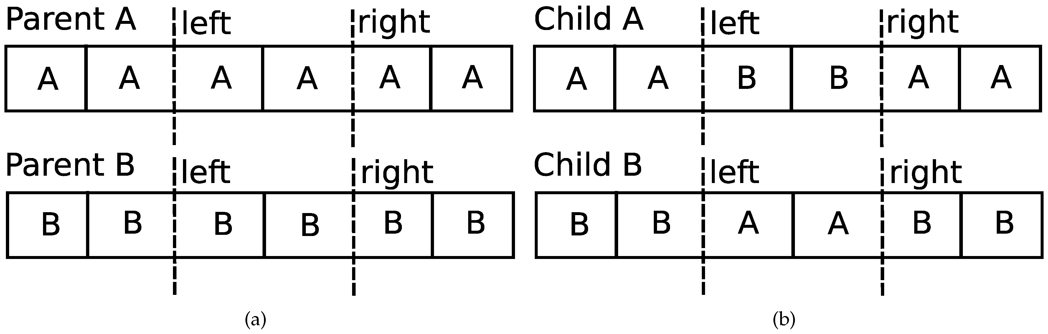
Figure 3.
Overview of the co-evolutionary system.
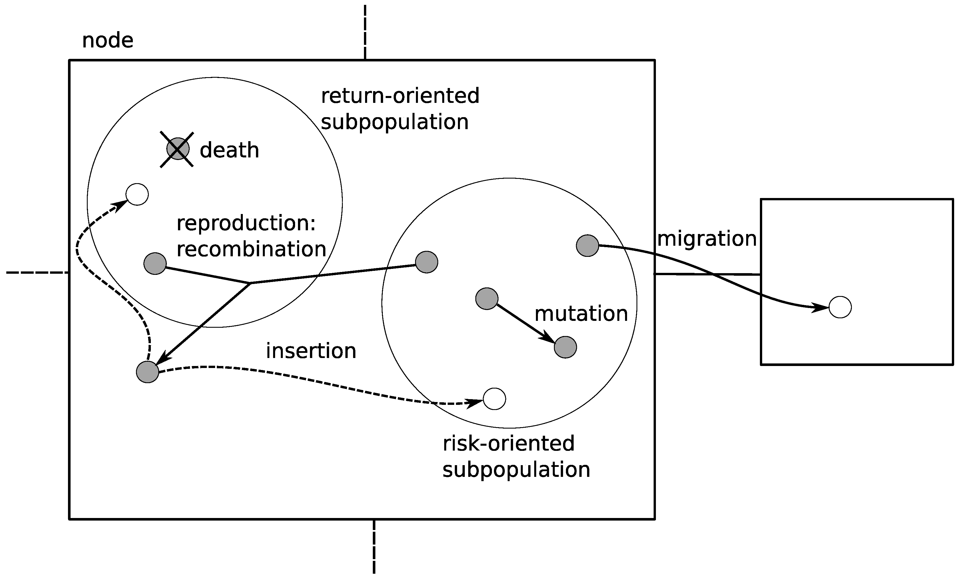
Figure 4.
Overview of co-evolutionary multi-agent system (CoEMAS).
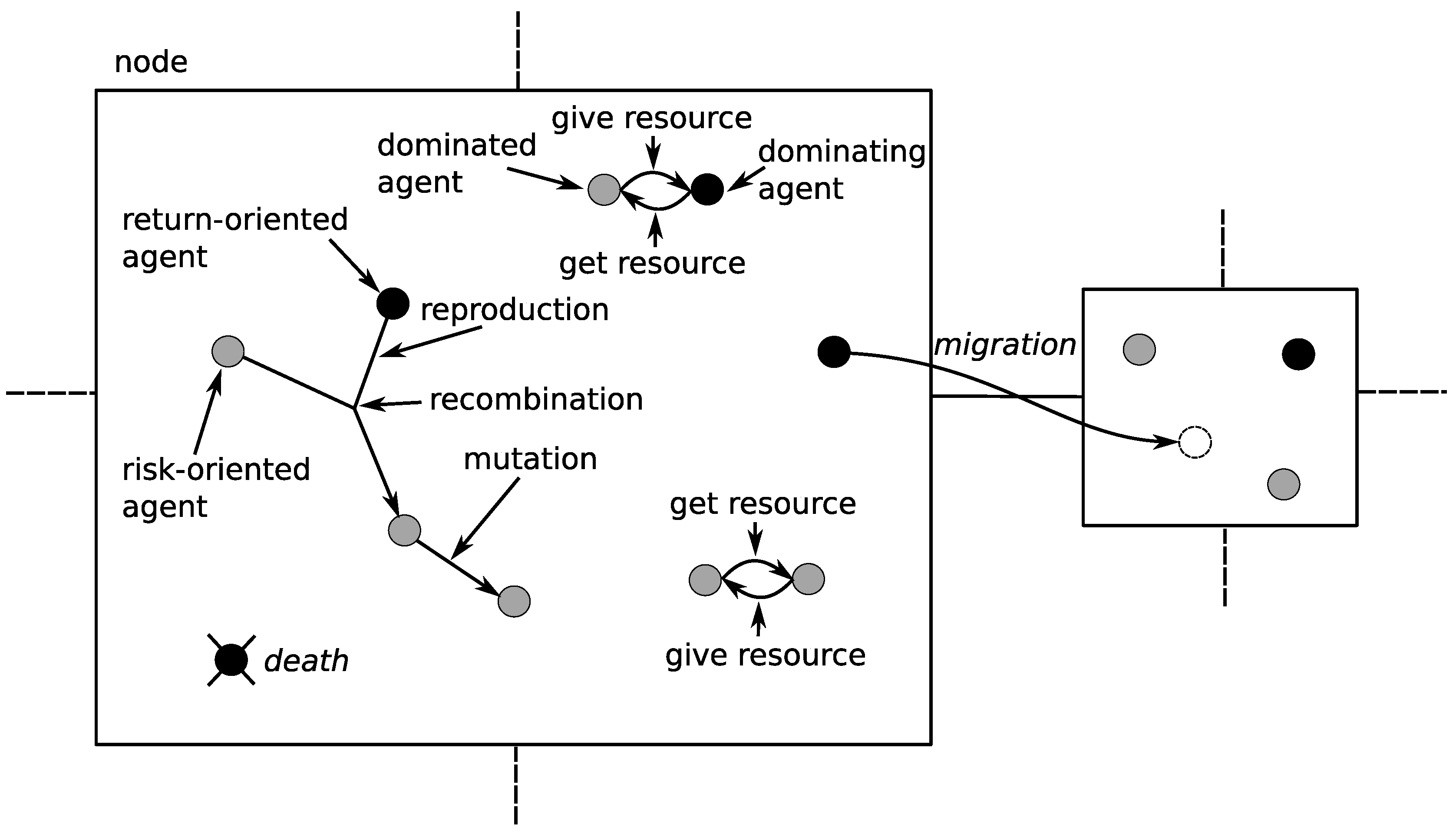
Figure 5.
Simple example of how trend following works in practice [76].
Figure 5.
Simple example of how trend following works in practice [76].
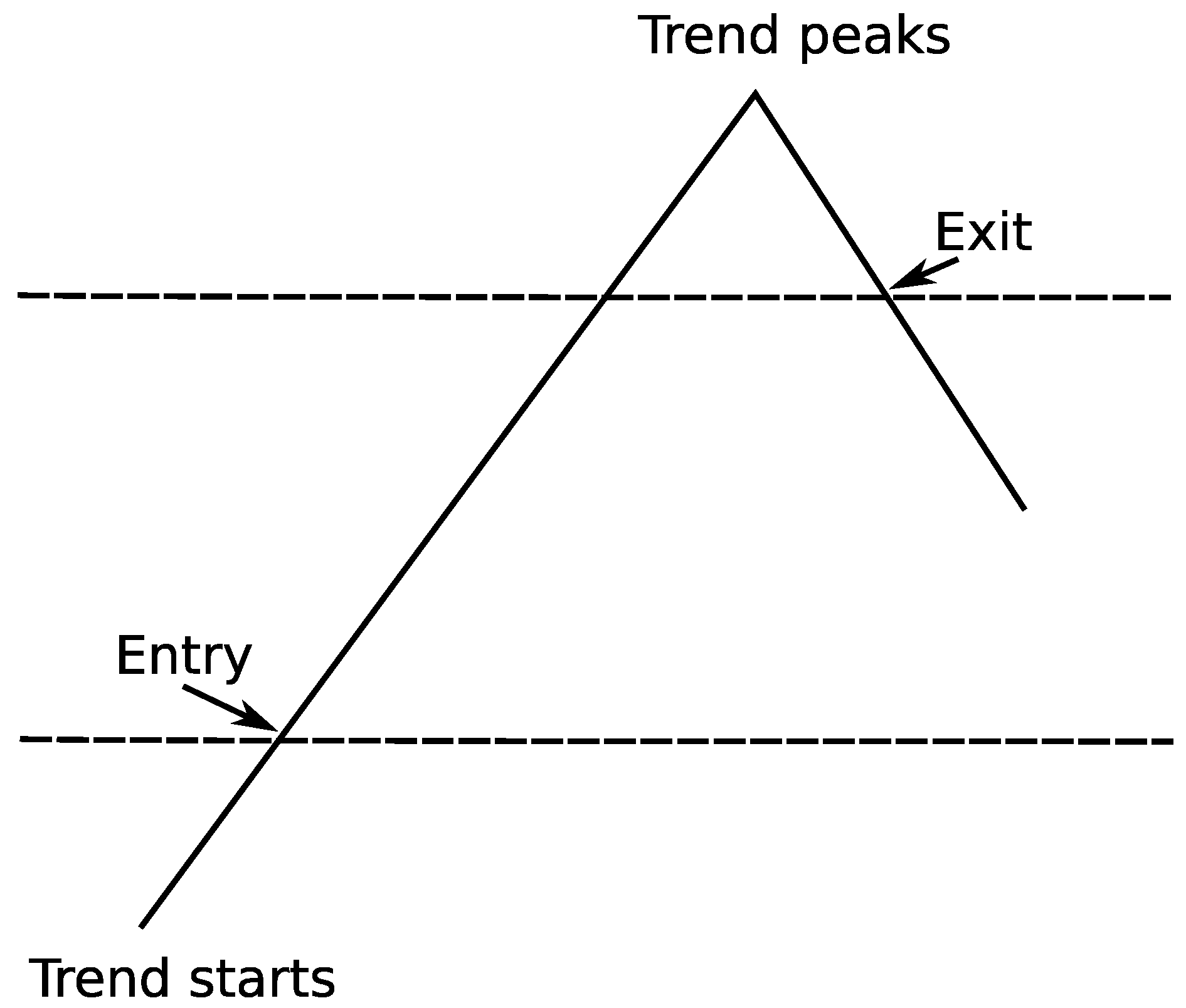
Figure 6.
Portfolio value in time for trend following (TF) using the short-term (a) and intermediate-term (b) trends.
Figure 6.
Portfolio value in time for trend following (TF) using the short-term (a) and intermediate-term (b) trends.

Figure 7.
Best (a) and average (b) portfolio values obtained for the genetic algorithm (GA).
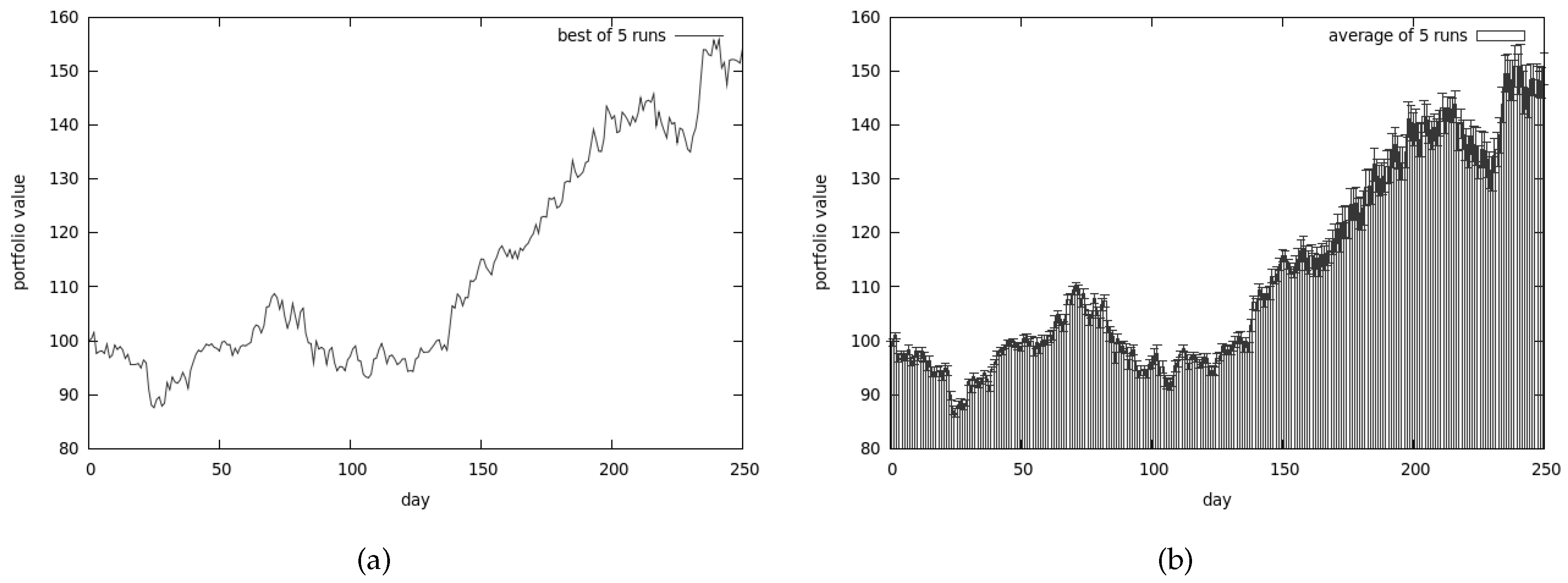
Figure 8.
Best (a) and average (b) portfolio values obtained for CEA.
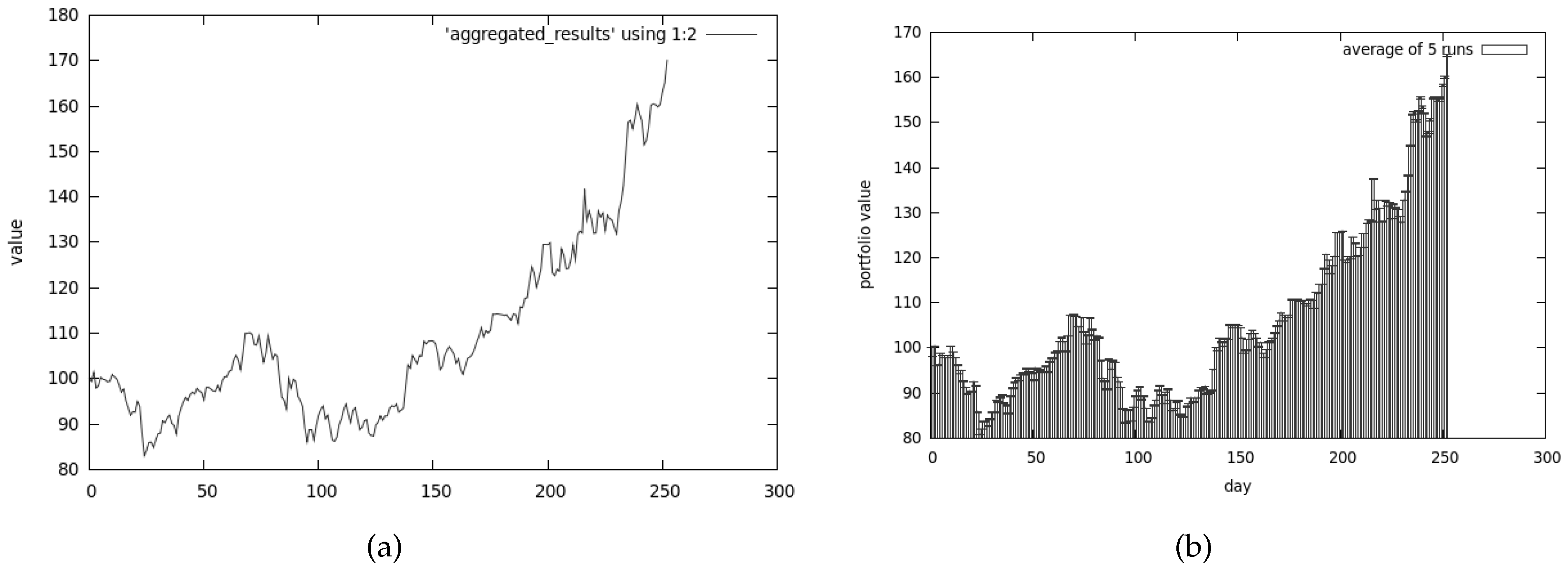
Figure 9.
Average value of risk in time for CEA.
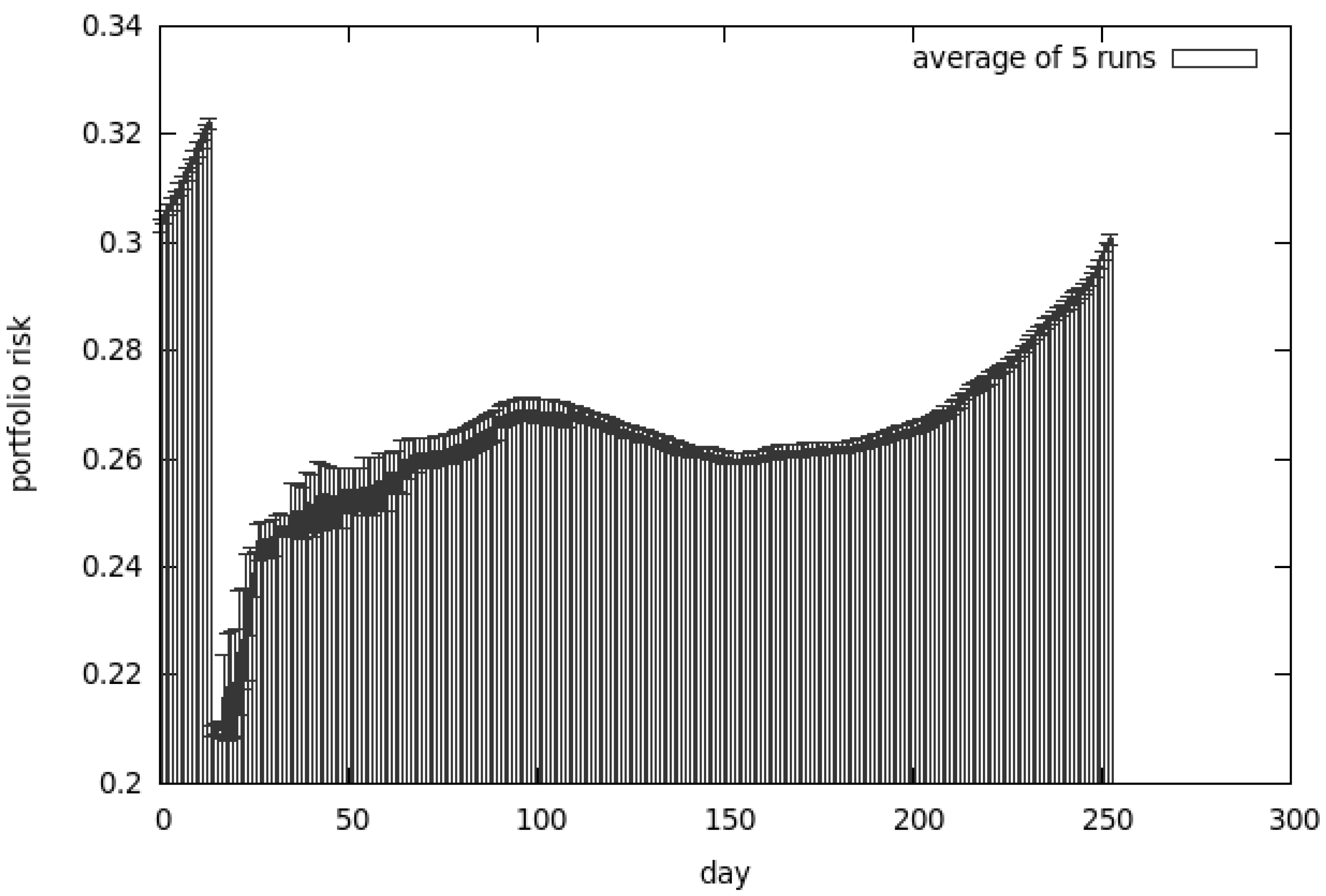
Figure 10.
Average portfolio value (a) and average risk value (b) for CoEMAS.

Figure 11.
Portfolio value in time for TF using short-term (a) and intermediate-term (b) trends.
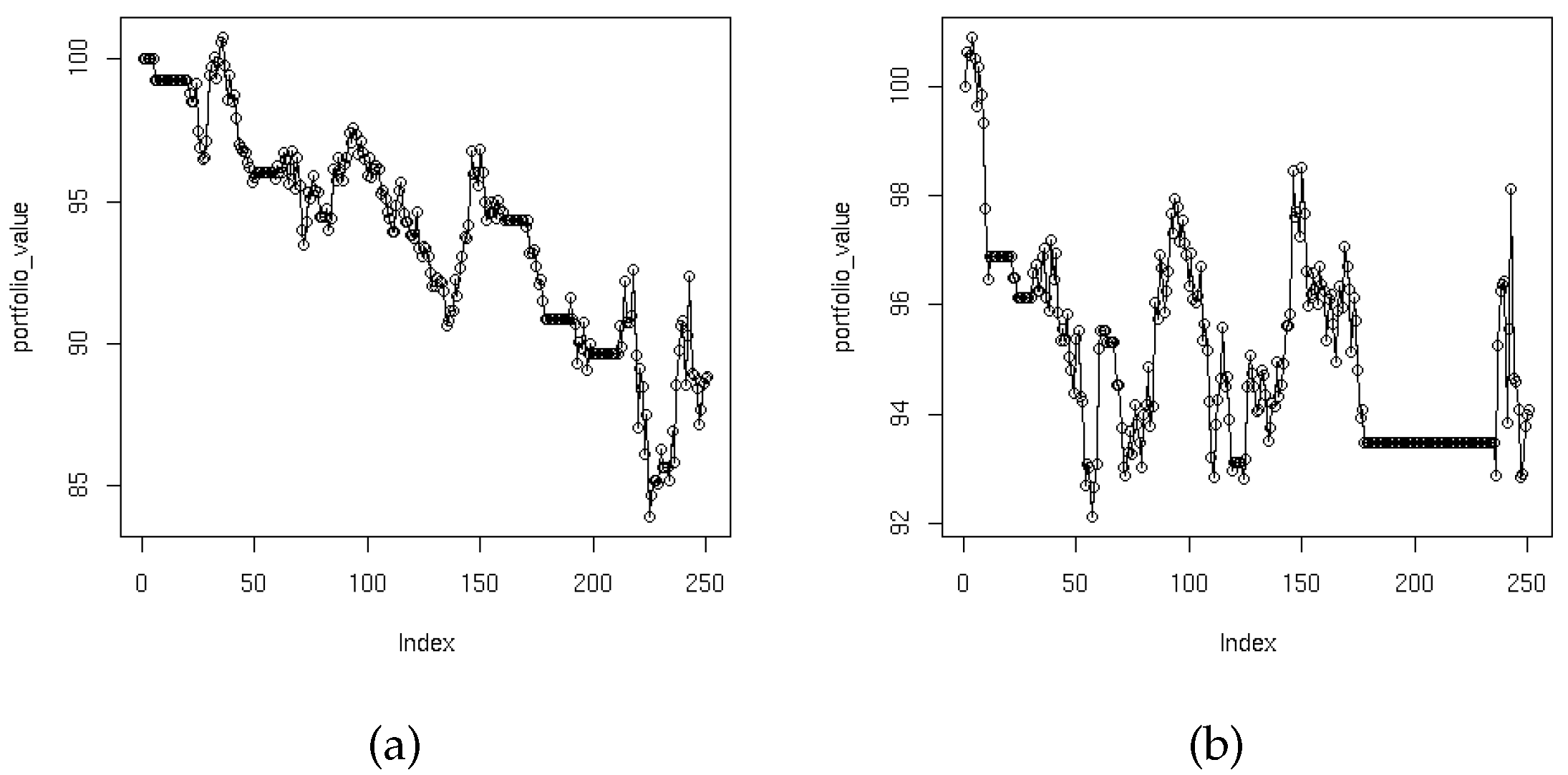
Figure 12.
Best (a) and average (b) portfolio value for the GA.

Figure 13.
Best (a) and average (b) portfolio value for CEA.

Figure 14.
Best (a) and average (b) portfolio value for CoEMAS.

Figure 15.
Average portfolio risk for CEA (a) and CoEMAS (b).
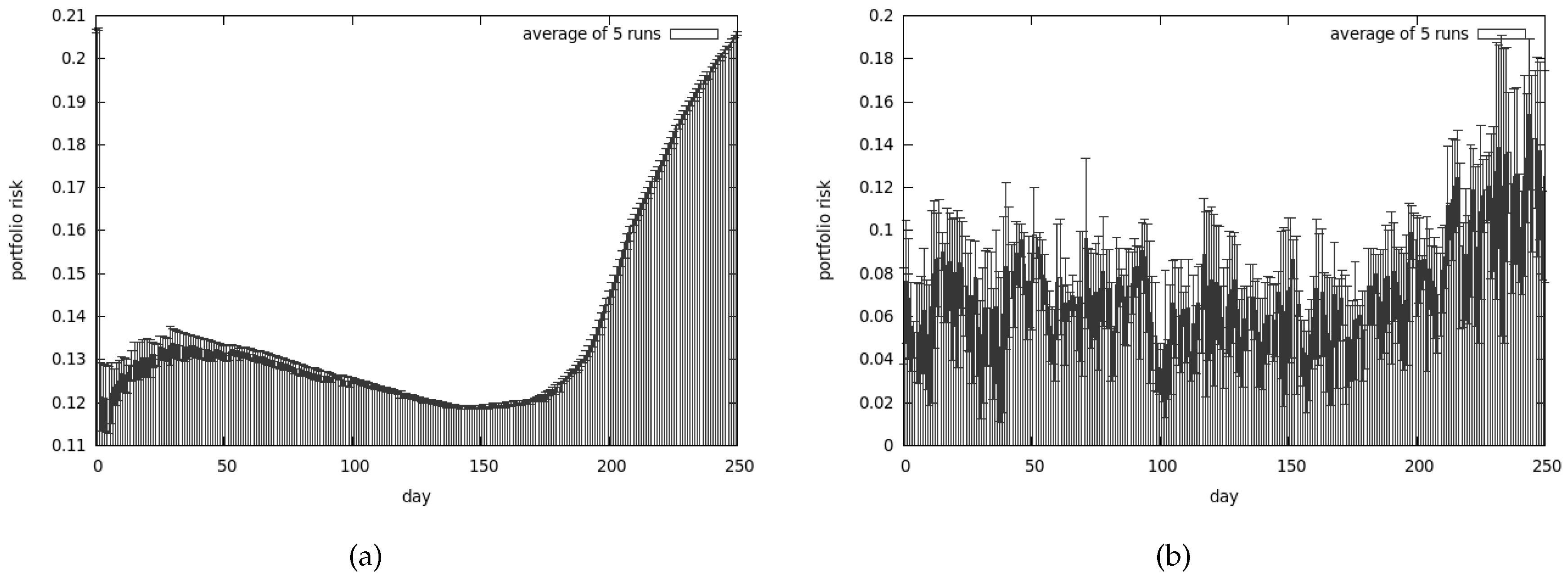
© 2017 by the authors. Licensee MDPI, Basel, Switzerland. This article is an open access article distributed under the terms and conditions of the Creative Commons Attribution (CC BY) license (http://creativecommons.org/licenses/by/4.0/).
Share and Cite
MDPI and ACS Style
Dreżewski, R.; Doroz, K. An Agent-Based Co-Evolutionary Multi-Objective Algorithm for Portfolio Optimization. Symmetry 2017, 9, 168. https://doi.org/10.3390/sym9090168
AMA Style
Dreżewski R, Doroz K. An Agent-Based Co-Evolutionary Multi-Objective Algorithm for Portfolio Optimization. Symmetry. 2017; 9(9):168. https://doi.org/10.3390/sym9090168
Chicago/Turabian StyleDreżewski, Rafał, and Krzysztof Doroz. 2017. "An Agent-Based Co-Evolutionary Multi-Objective Algorithm for Portfolio Optimization" Symmetry 9, no. 9: 168. https://doi.org/10.3390/sym9090168
Note that from the first issue of 2016, this journal uses article numbers instead of page numbers. See further details here.