A Novel Single-Valued Neutrosophic Set Similarity Measure and Its Application in Multicriteria Decision-Making

Abstract

The single-valued neutrosophic set is a subclass of neutrosophic set, and has been proposed in recent years. An important application for single-valued neutrosophic sets is to solve multicriteria decision-making problems. The key to using neutrosophic sets in decision-making applications is to make a similarity measure between single-valued neutrosophic sets. In this paper, a new method to measure the similarity between single-valued neutrosophic sets using Dempster–Shafer evidence theory is proposed, and it is applied in multicriteria decision-making. Finally, some examples are given to show the reasonable and effective use of the proposed method.

1. Introduction

The concept of a neutrosophic set, which generalizes the above-mentioned sets from philosophical point of view, was proposed by Smarandache [1] in 1999, and it is defined as a set about the degree of truth, indeterminacy, and falsity. According to the definition of a neutrosophic set, a neutrosophic set A in a universal set X is characterized independently by a truth-membership function $T_A\left(x\right)$, an indeterminacy-membership function $I_A\left(x\right)$, and a falsity-membership function $F_A\left(x\right)$, where in X are real standard or nonstandard subsets of ${]}^{-}0,1^{+}[$. However, the neutrosophic set generalizes the above-mentioned sets from a philosophical point of view. It is difficult to apply in practical problems. So, the concept of interval neutrosophic sets (INSs) [2] and single-valued neutrosophic sets (SVNSs) [3] were proposed by Wang et al. Because INS and SVNS are easy to express, and due to the fuzziness of subjective judgment, these two kinds of neutrosophic sets are widely used in reality, such as in multicriteria decision-making [4,5,6,7,8,9], image processing [10,11,12], medicine [13], fault diagnosis [14], and personnel selection [15]. Among them, decision-making is a hot issue of research for scholars in various fields [16,17].

This paper introduces how to measure the similarity between SVNSs, which is an important topic in the neutrosophic theory. Similarity measure is key in the SVNS application, and many similarity measures have been proposed by some researchers. In [18], the notion of distance between two SVNSs is introduced and entropy of SVNS is also defined by Majumdar and Samanta. In [6], Ye presented similarity measure of SVNSs using the weighted cosine. Then, in [5], a multicriteria decision-making method is introduced based on the two aggregation operators and cosine similarity measure for SVNSs. In [14], Ye presented two cotangent similarity measures for SVNSs based on cotangent function, and these similarity measures were applied in the fault diagnosis of a steam turbine. However, the cosine similarity measures defined [5,6] have some drawbacks. The results using cosine similarity measures are not consistent with intuition in some situations. Specific analysis will be presented in the following sections. Therefore, similarity measure is still an open problem.

In this paper, a new method of calculating the similarity between SVNSs using Dempster–Shafer (D–S) evidence theory is proposed and is applied in multicriteria decision-making. D–S evidence theory was first proposed by Dempster and then developed by Shafer, and has received recent attention in the field of information fusion. A significant advantage of D–S evidence theory over the traditional probability is that a better fusion result can be obtained via simple reasoning process without knowing the prior probability. In addition, an important property of this theory is that it can easily describe the uncertainty of information [19,20,21]. In recent years, a number of papers about further research in D–S evidence theory have been published. The main research topics include combination rule [22,23,24], basic probability assignment(BPA) approximation [25,26], distance of evidence [27,28], and BPA generation [29]. Besides, to solve the problem that frame of discernment is often not incomplete, the generalized evidence theory (GET) is proposed and now there are many studies on GET [30,31,32]. What is more, D–S evidence theory has been widely used in many fields, such as image fusion [33,34], sensor data fusion [35], gender profiling [36], device fault diagnosis [37,38], and so on [39,40,41,42,43]. In this paper, the method of measuring similarity between SVNSs is that SVNSs are first converted to the basic probability assignment(BPA). Then, the value of similarity measure between SVNSs can be obtained by computing the similarity of BPAs. The correlation between BPAs can be obtained by the correlation coefficient or the evidential distance [44] in D–S evidence theory. The correlation coefficient by Jiang [45] will be applied in our method to measure the similarity between the SVNSs. This correlation coefficient is one of the coefficients which can effectively measure the similarity or relevance of evidence. Finally, the new SVNSs similarity measure method-based D–S evidence theory is used in multicriteria decision-making for single-valued neutrosophic sets, and some examples are given to show its effectiveness.

The remainder of this paper is organized as follows: Section 2 introduces the theoretical background of this research. The method which measures the similarity between SVNSs using D–S evidence theory is introduced in Section 3. Next, compared with existing methods, some tests and analysis are given in Section 4. Finally, D–S evidence theory is applied in multicriteria decision-making under SVNS in Section 4 and we present our conclusions in Section 6.

2. Preliminaries

2.1. Neutrosophic Sets

The definition of a neutrosophic set as proposed by Smarandache [1] is as follows.

Definition 1.

Let X be a space of points (objects), with a generic element in X denoted by x. A neutrosophic set A in X is characterized by a truth-membership function $T_A$, an indeterminacy membership function $I_A$, and a falsity membership function $F_A$. $T_A\left(x\right)$, $I_A\left(x\right)$, and $F_A\left(x\right)$ are real standard or non-standard subsets of $]0^{-},1^{+}[$. That is

$$\begin{array}{c}{T}_A:X\to ]0^{-},1^{+}[\hfill \\ I_A:X\to ]0^{-},1^{+}[\hfill \\ F_A:X\to ]0^{-},1^{+}[\hfill \end{array}$$

(1)

There is no restriction on the sum of $T_A\left(x\right)$, $I_A\left(x\right)$, and $F_A\left(x\right)$, so $0^{-}\le sup{T}_A\left(x\right)+sup{I}_A\left(x\right)+sup{F}_A\left(x\right)\le 3^{+}$.

Definition 2.

The complement of a neutrosophic set A is denoted by c(A), and is defined by

$$\begin{array}{c}{T}_{c\left(A\right)}\left(x\right)=\left\{1^{+}\right\}-T_A\left(x\right)\hfill \\ I_{c\left(A\right)}\left(x\right)=\left\{1^{+}\right\}-I_A\left(x\right)\hfill \\ F_{c\left(A\right)}\left(x\right)=\left\{1^{+}\right\}-F_A\left(x\right)\hfill \end{array}$$

(2)

where all x is in X.

Definition 3.

A neutrosophic set A is contained in the other neutrosophic set B, $A\subseteq B$, if and only if

$$\begin{array}{c}inf{T}_A\left(x\right)\le inf{T}_B\left(x\right),sup{T}_A\left(x\right)\le sup{T}_B\left(x\right)\hfill \\ inf{F}_A\left(x\right)\le inf{F}_B\left(x\right),sup{F}_A\left(x\right)\le sup{F}_B\left(x\right)\hfill \end{array}$$

(3)

where all x is in X.

Definition 4.

The union of two neutrosophic sets A and B is a neutrosophic set C, written as $C=A\cup B$, whose truth-membership, indeterminacy membership, and falsity membership functions are related to those of A and B by

$$\begin{array}{c}{T}_C\left(x\right)=T_A\left(x\right)+T_B\left(x\right)-T_A\left(x\right)\times T_B\left(x\right)\hfill \\ I_C\left(x\right)=I_A\left(x\right)+I_B\left(x\right)-I_A\left(x\right)\times I_B\left(x\right)\hfill \\ F_C\left(x\right)=F_A\left(x\right)+F_B\left(x\right)-F_A\left(x\right)\times F_B\left(x\right)\hfill \end{array}$$

(4)

where all x is in X.

Definition 5.

The intersection of two neutrosophic sets A and B is a neutrosophic set C, written as $C=A\cap B$, whose truth-membership, indeterminacy membership, and falsity membership functions are related to those of A and B by

$$\begin{array}{c}{T}_C\left(x\right)=T_A\left(x\right)\times T_B\left(x\right)\hfill \\ I_C\left(x\right)=I_A\left(x\right)\times I_B\left(x\right)\hfill \\ F_C\left(x\right)=F_A\left(x\right)\times F_B\left(x\right)\hfill \end{array}$$

(5)

where all x is in X.

2.2. Single-Valued Neutrosophic Set

The definition of SVNS [3] and the weighted aggregation operators of SVNS [5] are introduced as follows:

Definition 6.

[3] Let X be a space of points (objects), with a generic element in X denoted by x. A single-valued neutrosophic set (SVNS) A in X is characterized by truth-membership function $T_A$, indeterminacy-membership function $I_A$, and falsity-membership function $F_A$, For each point x in X, $T_A\left(x\right),I_A\left(x\right),F_A\left(x\right)\in [0,1]$. Then, a simplification of the neutrosophic set A is denoted by

$$A=\left\{〈x,T\left(x\right),I\left(x\right),F\left(x\right)〉\right|x\in X\}$$

(6)

It is a subclass of neutrosophic sets. In this paper, for the sake of simplicity, the SVNS $A=\left\{〈x,T\left(x\right),I\left(x\right),F\left(x\right)〉\right|x\in X\}$ is denoted by the simplified symbol $A=\left\{〈T\left(x\right),I\left(x\right),F\left(x\right)〉\right|x\in X\}$.

Definition 7.

[3] The complement of an SVNS A is denoted by c(A), and is defined:

$$\begin{array}{c}{T}_{c\left(A\right)}\left(x\right)=F_A\left(x\right)\hfill \\ I_{c\left(A\right)}\left(x\right)=1-I_A\left(x\right)\hfill \\ F_{c\left(A\right)}\left(x\right)=T_A\left(x\right)\hfill \end{array}$$

(7)

where all x is in X.

Definition 8.

[3] An SVNS A is contained in the other SVNS B, $A\subseteq B$, if and only if $T_A\left(x\right)\le T_B\left(x\right),I_A\left(x\right)\ge I_B\left(x\right),F_A\left(x\right)\ge F_B\left(x\right)$.

Definition 9.

[3] Two SVNSs A and B are equal, written as $A=B$ if and only if $A\subseteq B$ and $B\subseteq A$.

Definition 10.

[5] Let A, B be two SVNSs. Operational relations are defined by

$$\begin{array}{cc}\hfill A+B=& \hfill 〈T_A\left(x\right)+T_B\left(x\right)-T_A\left(x\right)T_B\left(x\right),\\ & \hfill I_A\left(x\right)+I_B\left(x\right)-I_A\left(x\right)I_B\left(x\right),\\ & \hfill F_A\left(x\right)+F_B\left(x\right)-F_A\left(x\right)F_B\left(x\right)〉\end{array}$$

(8)

$$A·B=〈T_A\left(x\right)T_B\left(x\right),I_A\left(x\right)I_B\left(x\right),F_A\left(x\right)F_B\left(x\right)〉$$

(9)

$$\lambda A=〈1-{(1-T_A\left(x\right))}^{\lambda },1-{(1-I_A\left(x\right))}^{\lambda },1-{(1-F_A\left(x\right))}^{\lambda }〉,\lambda >0$$

(10)

$$A^{\lambda }=〈T_A^{\lambda }\left(x\right),I_A^{\lambda }\left(x\right),F_A^{\lambda }\left(x\right)〉,\lambda >0$$

(11)

Definition 11.

[5] Let $A_j(j=1,2,\dots ,n)$ be an SVNS. The simplified neutrosophic weighted arithmetic average operator is defined by

$$F_w(A_1,A_2,\dots ,A_n)=\sum _{j=1}^n{w}_j{A}_j$$

(12)

where $W=(w_1,w_2,\dots ,w_n)$ is the weight vector of $A_j(j=1,2,\dots ,n),w_j\in [0,1]$ and ${\displaystyle \sum _{j=1}^n}{w}_j=1$

2.3. Dempster–Shafer Evidence Theory

The Dempster–Shafer (D–S) evidence theory was introduced by Dempster and then developed by Shafer, and has emerged from their works on statistical inference and uncertain reasoning.

Definition 12.

In D–S evidence theory, there is a fixed set of N mutually exclusive and exhaustive elements, called the frame of discernment. Let $\mathsf{\Theta }$ be a set, indicated by

$$\mathsf{\Theta }=\{{\theta }_1,{\theta }_2,\cdots {\theta }_i,\cdots ,{\theta }_N\}.$$

(13)

Let us denote $P\left(\mathsf{\Theta }\right)$ as the power set composed of $2^N$ elements of $\mathsf{\Theta }$

$$P\left(\mathsf{\Theta }\right)=\{\varnothing ,\left\{{\theta }_1\right\},\cdots \left\{{\theta }_N\right\},\{{\theta }_1,{\theta }_2\},\cdots ,\{{\theta }_1,{\theta }_2,\cdots {\theta }_i\},\cdots ,\mathsf{\Theta }\}.$$

(14)

Definition 13.

A mass function is a mapping m from $P\left(\mathsf{\Theta }\right)$ to [0,1], formally defined by:

$$m:P\left(\mathsf{\Theta }\right)\to [0,1],A\to m\left(A\right)$$

(15)

which satisfies the following condition:

$$m(\varnothing )=0$$

(16)

$$\sum _{A\in P\left(\mathsf{\Theta }\right)}m\left(A\right)=1.$$

(17)

A represents any one of the elements in the $P\left(\mathsf{\Theta }\right)$. The mass $m\left(A\right)$ represents how strongly the evidence supports A. When m(A)>0, A, which is a member of the power set, is called a focal element of the mass function.

Definition 14.

In D–S evidence theory, a mass function is also called a basic probability assignment (BPA). Let us assume there are two BPAs, operating on two sets of propositions B and C, respectively, indicated by $m_1$ and $m_2$. The Dempster’s combination rule is used to combine them as follows:

$$m\left(A\right)=\left\{\begin{array}{c}0,\hfill \\ \frac{1}{1-K}{\displaystyle \sum _{B\cap C=A}}{m}_1\left(B\right)m_2\left(C\right)\end{array}\right.\begin{array}{c}A=\varnothing \\ A\ne \varnothing \end{array}$$

(18)

$$K=\sum _{B\cap C=\varnothing }{m}_1\left(B\right)m_2\left(C\right),$$

(19)

In Equations (18) and (19), K shows the conflict between the two BPAs $m_1$ and $m_2$.

2.4. A Correlation Coefficient

In order to measure the similarity between two BPAs, a correlation coefficient of belief functions is proposed in [45], detailed as follows:

Definition 15.

For a discernment frame $\mathsf{\Theta }$ with N elements, suppose the mass of two pieces of evidence denoted by $m_1$, $m_2$. The correlation coefficient is defined as:

$$r_{BPA}\left(m_1,m_2\right)=\frac{c\left(m_1,m_2\right)}{\sqrt{c\left(m_1,m_1\right)·c\left(m_2,m_2\right)}}$$

(20)

where the correlation coefficient $r_{BPA}\in [0,1]$ and $c(m_1,m_2)$ is the degree of correlation denoted as:

$$c(m_1,m_2)=\sum _{i=1}^{2^N}\sum _{j=1}^{2^N}{m}_1\left(A_i\right)m_2\left(A_j\right)\frac{\left|A_i\cap A_j\right|}{\left|A_i\cup A_j\right|}$$

(21)

where $i,j=1,\cdots ,2^N$; $A_i$, $A_j$ are the focal elements of mass, and $\left|·\right|$ is the cardinality of a subset.

When the two BPAs are different absolutely, the degree of difference should be the least, which is 0. When the two BPAs are consistent absolutely, the result of the correlation coefficient is 1.

3. A New Similarity Measures for SNVS

The idea of the new similarity measure is that SNVSs can be converted to BPAs and the similarity measure between the two SNVSs be obtained by computing the correlation coefficient between the two BPAs by Equations (20) and (21). The innovation of our method is that a reasonable method for converting SVNS to BPA is proposed and the new idea of using correlation coefficients by Jiang [45] to measure similarity between SNVSs. The key of this method is to find the connection between SNVSs and BPA. In other words, finding a way to generate the BPA reasonably is very important.

Definition 16.

Suppose neutrosophic set A is an SNVS. A simplification of the neutrosophic set A is denoted by $A=\left\{〈T_A\left(x\right),I_A\left(x\right),F_A\left(x\right)〉\right|x\in X\}$. Each point x is in X and $T_A\left(x\right)$,$I_A\left(x\right)$, $F_A\left(x\right)\in [0,1]$. According to the meaning of SNVS and D–S evidence theory, the frame of discernment can be defined $\mathsf{\Theta }=\{T_x,F_x\}$. $T_x$ and $F_x$ represent the trust for x and the opposition for x respectively. Subset $\{T_x,F_x\}$ of $\mathsf{\Theta }$ represents supporting for both $T_x$ and $F_x$. In other words, it means choice between $T_x$ and $F_x$ cannot be made. So, the power set $\mathrm{P}\left(\mathsf{\Theta }\right)$ is $\{\varnothing ,\left\{T_x\right\},\left\{F_x\right\},\{T_x,F_x\}\}$. The BPA can be defined $m_A(\varnothing )$, $m_A\left(T_x\right)$, $m_A\left(F_x\right)$, $m_A(T_x,F_x)$. They respectively indicate the degree of the A support for ∅, $T_x$, $F_x$ and $T_x,F_x$.

Definition 17.

Suppose neutrosophic set A is an SNVS. A simplification of the neutrosophic set A is denoted by $A=\left\{〈T_A\left(x\right),I_A\left(x\right),F_A\left(x\right)〉\right|x\in X\}$. Each point x is in X and $T_A\left(x\right)$, $I_A\left(x\right)$, $F_A\left(x\right)\in [0,1]$. The relationship between SVNS and BPA can be expressed as follows:

$$\begin{array}{c}{m}_A\left(T\right)=T_A\left(x\right)/(T_A\left(x\right)+F_A\left(x\right)+(1-I_A\left(x\right)))\hfill \\ m_A\left(F\right)=F_A\left(x\right)/(T_A\left(x\right)+F_A\left(x\right)+(1-I_A\left(x\right)))\hfill \\ m_A(T,X)=(1-I_A\left(x\right))/(T_A\left(x\right)+F_A\left(x\right)+(1-I_A\left(x\right)))\hfill \end{array}$$

(22)

$T_A\left(x\right)$ represents the degree of the trust for x. Similarly, $m_A\left(T_x\right)$ can also express the degree of the trust for x. $T_A\left(x\right)$ and $m_A\left(F_x\right)$ both represent the degree of the opposition for x. So, $m_A\left(T_x\right)=T_A\left(x\right)$ and $m_A\left(F_x\right)=F_A\left(x\right)$ are defined when generating the BPA according to the SNVS. $I_A\left(x\right)$ indicates the degree of support for other, with the exception of trust and opposition. So, $1-I_A\left(x\right)$ expresses the degree of trust for x and opposition for x. The meaning of $m_A(T_x,F_x)$ is the same as $1-I_A\left(x\right)$. So, $m_A(T_x,F_x)=1-I_A\left(x\right)$ is defined in Equation (22). We can see that using basic probability assignment (BPA) can express the SNVS reasonably.

The new method to calculate the similarity between two SVNSs is presented as follows:

Assume that two SVNSs A and B are denoted by $A=\left\{〈T_A\left(x\right),I_A\left(x\right),F_A\left(x\right)〉\right|x\in X\}$, $B=\left\{〈T_B\left(x\right),I_B\left(x\right),F_B\left(x\right)〉\right|x\in X\}$.

• Step 1: According to A and B, two groups of BPAs $m_A$ and $m_B$ can be obtained by Equation (22);
• Step 2: Compute correlation coefficient $r_{BPA}$ between $m_A$ and $m_B$ by Equations (20) and (21);
• Step 3: The similarity measure $S_r(A,B)$ can be obtained as:

  $$S_r(A,B)=r_{BPA}(m_A,m_B)$$

In the following, one example is used to show the steps of our proposed method.

Example 1.

Suppose two SVNSs A and B in $X=x$. The value of A is <0.7 0.8 0.2> and the value of B is <0.6 0.8 0.1>. Calculating similarity using D–S evidence theory is as follows.

• Step 1: According to A and B of SVNS, we can know

  $$T_A\left(x\right)=0.7,I_A\left(x\right)=0.8,F_A\left(x\right)=0.2$$

  $$T_B\left(x\right)=0.6,I_B\left(x\right)=0.8,F_B\left(x\right)=0.1$$
  So, two groups of BPAs $m_A$ and $m_B$ can be obtained by Equation (22).

  $$\begin{gathered} m_A(\varnothing )=0, \\ {m}_A\left(T_x\right)=T_A\left(x\right)/(T_A\left(x\right)+F_A\left(x\right)+(1-I_A\left(x\right)))=0.6364, \\ {m}_A\left(F_x\right)=T_A\left(x\right)/(T_A\left(x\right)+F_A\left(x\right)+(1-I_A\left(x\right)))=0.1818, \\ {m}_A(T_x,F_x)=T_A\left(x\right)/(T_A\left(x\right)+F_A\left(x\right)+(1-I_A\left(x\right)))=0.1818 \end{gathered}$$

  $$\begin{gathered} m_B(\varnothing )=0, \\ {m}_B\left(T_x\right)=T_B\left(x\right)/(T_B\left(x\right)+F_B\left(x\right)+(1-I_B\left(x\right)))=0.6667, \\ {m}_B\left(F_x\right)=T_B\left(x\right)/(T_B\left(x\right)+F_B\left(x\right)+(1-I_B\left(x\right)))=0.1111, \\ {m}_B(T_x,F_x)=T_B\left(x\right)/(T_B\left(x\right)+F_B\left(x\right)+(1-I_B\left(x\right)))=0.2222 \end{gathered}$$
• Step 2: Compute correlation coefficient $r_{BPA}$ between $m_A$ and $m_B$ by Equations (20) and (21). Firstly, we can get the c by Equation (21).

  $$c(m_A,m_A)=0.5500, c(m_B,m_B)=0.7500, c(m_A,m_B)=0.6400$$
  Then, $r_{BPA}$ can be obtained by Equation (20).

  $$r_{BPA}(m_A,m_B)=0.9965$$
• Step 3: The similarity measure of SNVSs can be obtained as

  $$S_r(A,B)=0.9965.$$

4. Test and Analysis

In this section, to compare the similarity measures with existing similarity measures [6], the examples to demonstrate the effectiveness and rationality of similarity measures proposed of SVNSs is provided.

Example 2.

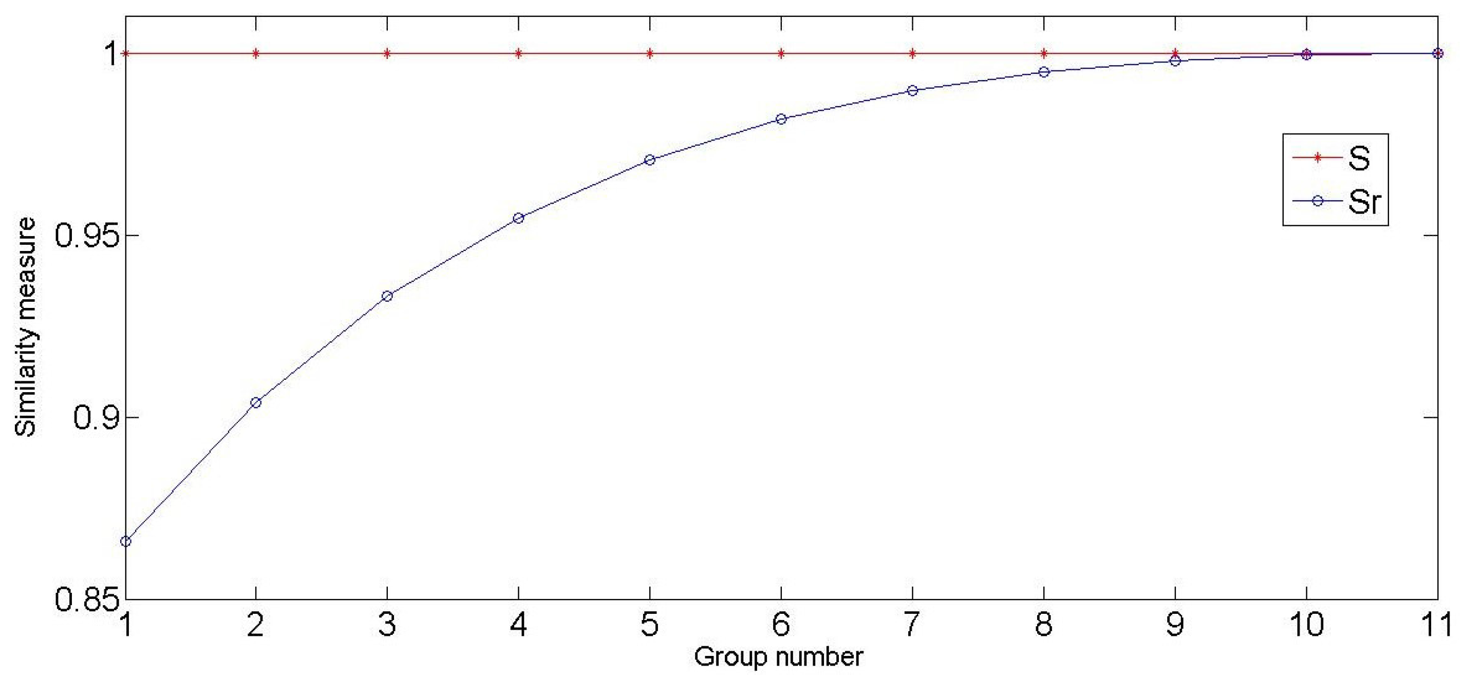
Suppose two SVNSs A and B in $X=x$. In this example, the value of A remains the unchanged, which is <1 0 0>. Meanwhile, $T_B\left(x\right)$ in B increased gradually. The similarity measures are computed by the method proposed by Ye’s method [6] and our method, respectively, and the results are shown in

Table 1. Similarity measure values.

Group Number	A	B	${\mathit{S}}_{\mathit{r}}$	S [6]
1	<1 0 0>	<0 0 0>	0.8660	1
2	<1 0 0>	<0.1 0 0>	0.9042	1
3	<1 0 0>	<0.2 0 0>	0.9333	1
4	<1 0 0>	<0.3 0 0>	0.9549	1
5	<1 0 0>	<0.4 0 0>	0.9707	1
6	<1 0 0>	<0.5 0 0>	0.9820	1
7	<1 0 0>	<0.6 0 0>	0.9897	1
8	<1 0 0>	<0.7 0 0>	0.9948	1
9	<1 0 0>	<0.8 0 0>	0.9979	1
10	<1 0 0>	<0.9 0 0>	0.9995	1
11	<1 0 0>	<1 0 0>	1	1

and Figure 1.

From Table 1 and Figure 1, we can see that our result is gradually increasing with the change of B. However, the similarity measure remains unchanged by Ye’s method. Obviously, Ye’s results are not consistent with intuition. With the growth of B, A and B are becoming more and more similar. In other words, the trend of similarity should be changed from small to large in this example. Our results are consistent with the intuitive analysis.

Example 3.

Suppose two SVNSs A and B in $X=x$ and we compare similarity measures using D–S evidence theory with similarity measure using [6]. The comparison results of similarity measure are shown in

Table 2. Similarity measure values.

Group Number	A	B	${\mathit{S}}_{\mathit{r}}$	S [6]
1	<0.6 0.2 0.8>	<0.3 0.1 0.4>	0.9862	1
2	<0.7 0.8 0.2>	<0.6 0.8 0.1>	0.9965	0.9935
3	<0.2 0.1 0.5>	<0.2 0.1 0.5>	1	1
4	<0.9 0.8 0.7>	<0.1 0.2 0.1>	0.8440	0.9379

.

In Example 3, SVNSs of the four groups were calculated and the results are shown in Table 2. From the analysis of data, we can see that the similarity measures of all SVNSs can be obtained reasonably by our method. However, Ye’s result is not consistent with intuition in group 1.

5. Multicriteria Decision-Making

In this section, the similarity measure we proposed is applied to solve multicriteria decision-making problems.

Assume that there are multiple groups of alternatives, which can be expressed as $A_1,A_2,\dots ,A_{\mathrm{m}}$. $C_1,C_2,\dots ,C_n$ is expressed as N criteria. In the decision process, the evaluation information of the alternative $A_i$ on the criteria is represented in the form of an SVNS:

$$A_{\mathrm{i}}=〈C_j,T_{A_i}\left(C_j\right),I_{A_i}\left(C_j\right),F_{A_i}\left(C_j\right)〉.$$

(23)

where $A_i\in \{A_1,A_2,\dots ,A_m\}$, $C_j\in \{C_1,C_2,\dots ,C_n\}$ and $0\le T_{A_i}\left(C_j\right)\le 1,0\le I_{A_i}\left(C_j\right)\le 1,0\le F_{A_i}\left(C_j\right)\le 1$. Besides, the importance of each criterion is expressed as $w_1,w_2,\dots ,w_n$, which is $w_j\in [0,1]$ and ${\displaystyle \sum _{j=1}^n}{w}_j=1$. For convenience, Equation (23) is denoted by ${\alpha }_{ij}=〈t_{ij},i_{ij},f_{ij}〉,(i=1,2,\dots ,m;j=1,2,\dots ,n)$. D can be obtained as folloTherefore, simplified neutrosophic decision matrixws:

$$\begin{array}{c}\hfill \begin{array}{c}D=\left[\begin{array}{cccc}{\alpha }_{11}& {\alpha }_{12}& \dots & {\alpha }_{1n}\\ {\alpha }_{21}& {\alpha }_{22}& \dots & {\alpha }_{2n}\\ \dots & \dots & \dots & \dots \\ {\alpha }_{m1}& {\alpha }_{m2}& \dots & {\alpha }_{mn}\end{array}\right]=\hfill \\ \left[\begin{array}{ccc}〈t_{11},i_{11},f_{11}〉& \dots & 〈t_{1n},i_{1n},f_{1n}〉\\ \dots & \dots & \dots \\ 〈t_{m1},i_{m1},f_{m1}〉& \dots & 〈t_{mn},i_{mn},f_{mn}〉\end{array}\right]\hfill \end{array}\end{array}$$

(24)

Then, the simplified neutrosophic value ${\alpha }_i$ for $A_i$ is ${\alpha }_i=〈t_i,i_i,f_i〉=F_{\mathrm{i}w}({\alpha }_{i1},{\alpha }_{i2},\dots ,{\alpha }_{in})$ by Equation (12) according to each row in the simplified neutrosophic decision matrix D.

In order to find the best alternative in all existing alternatives ${\alpha }_i(i\in 1,2,\dots ,m)$, the similarity measure needs to be computed between the alternative ${\alpha }_i$ and ideal alternative ${\alpha }^{*}$ by Equation (20) individually. Through the similarity measure between each alternative and the ideal alternative ${\alpha }^{*}$, the ranking order of all alternatives can be determined. The largest value of similarity measures is the best alternative in all existing alternatives. In other words, the greater the similarity measure is, the closer it is to the ideal alternative.

An example for a multicriteria decision-making problem of engineering alternatives is used as a demonstration to show the effectiveness of the similarity measure proposed in this paper.

Example 4.

Let us consider the decision-making problem adapted from [5]. There is an investment company which wants to invest a sum of money in the best option. There is a panel with four possible alternatives to invest the money: (1) $A_1$ is a car company; (2) $A_2$ is a food company; (3) $A_3$ is a computer company; (4) $A_4$ is an arms company. The investment company must take a decision according to the following three criteria: (1) $C_1$ is the risk analysis; (2) $C_2$ is the growth analysis; (3) $C_3$ is the environmental impact analysis. Then, the weight vector of the criteria is given by $W=(0.35,0.25,0.4)$, where the value of W is given according to the importance of three criteria. Ideal alternative ${\alpha }^{*}=〈1,0,0〉$.

Four investment plans $A_1$, $A_2$, $A_3$, $A_4$ were scored by an expert. For example, when we ask the opinion of an expert about investment in a car company in terms of the risk, they may say that the possibility in which the statement is good is 0.4. The possibility in which the statement is poor is 0.3, and the degree to which they are not sure is 0.2. The opinion of the expert can be expressed as ${\alpha }_{11}=〈0.4,0.2,0.3〉$. Thus, all information given by the expert is represented by a simplified neutrosophic decision matrix D:

$$D=\left[\begin{array}{ccc}〈0.4,0.2,0.3〉& 〈0.4,0.2,0.3〉& 〈0.2,0.2,0.5〉\\ 〈0.6,0.1,0.2〉& 〈0.6,0.1,0.2〉& 〈0.5,0.2,0.2〉\\ 〈0.3,0.2,0.3〉& 〈0.5,0.2,0.3〉& 〈0.5,0.3,0.2〉\\ 〈0.7,0,0.1〉& 〈0.6,0.1,0.2〉& 〈0.4,0.3,0.2〉\end{array}\right]$$

The proposed method in Section 3 is applied to solve this problem separately according to the following computational procedure:

• Step 1: ${\alpha }_i(i=1,2,3,4)$ can be obtained by Equation (12). The computing results are:

  $$\begin{array}{c}{\alpha }_1=〈0.3268,0.2000,0.3881〉\hfill \\ {\alpha }_2=〈0.5627,0.1414,0.2000〉\hfill \\ {\alpha }_3=〈0.4375,0.2416,0.2616〉\hfill \\ {\alpha }_4=〈0.5746,0.1555,0.1663〉\hfill \end{array}$$
• Step 2: Correlation measure between each alternative ${\alpha }_i$ and the ideal alternative ${\alpha }^{*}$ were calculated by the method proposed in Section 3. The results are as follows:

  $$\begin{array}{c}{S}_r({\alpha }^{*},{\alpha }_1)=0.8975\hfill \\ S_r({\alpha }^{*},{\alpha }_2)=0.9745\hfill \\ S_r({\alpha }^{*},{\alpha }_3)=0.9510\hfill \\ S_r({\alpha }^{*},{\alpha }_4)=0.9804\hfill \end{array}$$
• Step 3: According to the results in the second step, the ranking order of four alternatives is:

  $$A_4>A_2>A_3>A_1$$

It can be seen from the results that $A_4$ is the closest to the ideal replacement. This result is consistent with the result of Ye [5]. This example shows that our method is effective and correct in general.

Example 5.

The application background of this example is the same as in Example 4. In this example, an expert gives different suggestions for investment. So, the value of simplified neutrosophic decision matrix D is changed. A new D matrix is given as follows:

$$D=\left[\begin{array}{ccc}〈0.001,0,0〉& 〈0.001,0,0〉& 〈0.001,0,0〉\\ 〈0.9,0,0.01〉& 〈0.95,0,0.05〉& 〈0.96,0,0.01〉\\ 〈0.3,0.2,0.3〉& 〈0.5,0.2,0.3〉& 〈0.5,0.3,0.2〉\\ 〈0.7,0.0,0.1〉& 〈0.6,0.1,0.2〉& 〈0.4,0.3,0.2〉\end{array}\right]$$

The final result of our method is:

$$\begin{array}{c}{S}_r({\alpha }^{*},{\alpha }_1)=0.8665\hfill \\ S_r({\alpha }^{*},{\alpha }_2)=0.9997\hfill \\ S_r({\alpha }^{*},{\alpha }_3)=0.9510\hfill \\ S_r({\alpha }^{*},{\alpha }_4)=0.9804\hfill \end{array}$$

The result calculated using the Ye’s method [5] is:

$$\begin{array}{c}\mathrm{S}({\alpha }^{*},{\alpha }_1)=1\hfill \\ \mathrm{S}({\alpha }^{*},{\alpha }_2)=0.9998\hfill \\ \mathrm{S}({\alpha }^{*},{\alpha }_3)=0.9510\hfill \\ \mathrm{S}({\alpha }^{*},{\alpha }_4)=0.9804\hfill \end{array}$$

According to results of our method , the ranking order of four alternatives is $A_4>A_2>A_3>A_1$; this result is reasonable and consistent with intuitive analysis. However, when the results of Ye are sorted, the ranking order of four alternatives is $A_1>A_2>A_4>A_3$. This is obviously not true. The reason is that the similarity measure between ${\alpha }_2$ and ${\alpha }^{*}$ is greater than the similarity measure between ${\alpha }_1$ and ${\alpha }^{*}$ by intuitive analysis, where ${\alpha }_1$ is $〈0.001,0,0〉$ and ${\alpha }_2$ is $〈0.9417,0,0.0202〉$.

Example 6.

This example shows steam turbine faults diagnosed using multi-attribute decision-making. In the vibration fault diagnosis of the steam turbine, the relation between the cause and the fault phenomena of the steam turbine has been investigated in [46]. For the vibration fault diagnosis problem of steam turbine, the fault diagnosis of the turbine realized by the frequency features—which are extracted from the vibration signals of the steam turbine—is a simple and effective method. In the fault diagnosis problem of the turbine, we consider a set of ten fault patterns $A=\{A_1\left(\mathrm{Unbalance}\right),A_2\left(\mathrm{Pneumatic}\mathrm{force}\mathrm{couple}\right),$$A_3\left(\mathrm{Offset}\mathrm{center}\right),A_4\left(\mathrm{Oil}-\mathrm{membrane}\mathrm{oscillation}\right),$$A_5\left(\mathrm{Radial}\mathrm{impact}\mathrm{friction}\mathrm{of}\mathrm{rotor}\right),$$A_6\left(\mathrm{Symbiosis}\mathrm{looseness}\right),$$A_7\left(\mathrm{Damage}\mathrm{of}\mathrm{antithrust}\mathrm{bearing}\right)$,$A_8\left(\mathrm{Surge}\right),$$A_9\left(\mathrm{Looseness}\mathrm{of}\mathrm{bearing}\mathrm{block}\right),$$A_{10}\left(\mathrm{Nonuniform}\mathrm{bearing}\mathrm{stiffness}\right)\}$ as the fault knowledge and a set of nine frequency ranges for different frequency spectrum $C=\{C_1(0.01-0.39f),$$C_2(0.4-0.49f),C_3\left(0.5f\right),$$C_4(0.51-0.99f),C_5\left(f\right),$$C_6\left(2f\right),C_7(3-5f),$$C_8\left(\mathrm{Odd}\mathrm{times}\mathrm{of}f\right),C_9\left\{\mathrm{High}\mathrm{frequency}>5f\right\}\}$ under operating frequency f as a characteristic set. Then, the information of the fault knowledge can be introduced from [14], which is shown in

Table 3. Fault knowledge with single-valued neutrosophic values.

${\mathit{A}}_{\mathit{i}}$(Fault Knowledge)	${\mathit{C}}_1$(0.01–0.39 f)	${\mathit{C}}_2$(0.4–0.49 f)	${\mathit{C}}_3\left(0.5\mathit{f}\right)$	${\mathit{C}}_4$(0.51–0.99 f)	${\mathit{C}}_5\left(\mathit{f}\right)$	${\mathit{C}}_6\left(2\mathit{f}\right)$	${\mathit{C}}_7$(3–5 f)	${\mathit{C}}_8$(Odd Times of f)	${\mathit{C}}_9$(High Frequency > 5 f)
$A_1$(unbalance)	<0 0 1>	<0 0 1>	<0 0 1>	<0 0 1>	<0.85 0.15 0>	<0.04 0.02 0.94>	<0.04 0.03 0.93>	<0 0 1>	<0 0 1>
$A_2$(pneumatic force couple)	<0 0 1>	<0.03 0.28 0.69>	<0.9 0.3 0.88>	<0.55 0.15 0.3>	<0 0 1>	<0 0 1>	<0 0 1>	<0 0 1>	<0.08 0.05 0.87>
$A_3$(offset center)	<0 0 1>	<0 0 1>	<0 0 1>	<0 0 1>	<0.3 0.28 0.42>	<0.40 0.22 0.38>	<0.08 0.05 0.87>	<0 0 1>	<0 0 1>
$A_4$(oil-membrane oscillation)	<0.09 0.22 0.89>	<0.78 0.04 0.18>	<0 0 1>	<0.08 0.03 0.89>	<0 0 1>	<0 0 1>	<0 0 1>	<0 0 1>	<0 0 1>
$A_5$(radial impact friction of rotor)	<0.09 0.03 0.88>	<0.09 0.02 0.89>	<0.08 0.04 0.88>	<0.09 0.03 0.88>	<0.18 0.03 0.79>	<0.08 0.05 0.87>	<0.08 0.05 0.87>	<0.08 0.04 0.88>	<0.08 0.04 0.88>
$A_6$(symbiosis looseness)	<0 0 1>	<0 0 1>	<0 0 1>	<0 0 1>	<0.18 0.04 0.78>	<0.12 0.05 0.83>	<0.37 0.08 0.55>	<0 0 1>	<0.22, 0.06, 0.72>
$A_7$(damage of antithrust bearing)	<0 0 1>	<0 0 1>	<0.08 0.04 0.88>	<0.86 0.07 0.07>	<0 0 1>	<0 0 1>	<0 0 1>	<0 0 1>	<0 0 1>
$A_8$(surge)	<0 0 1>	<0.27 0.05 0.68>	<0.08 0.04 0.88>	<0.54 0.08 0.38>	<0 0 1>	<0 0 1>	<0 0 1>	<0 0 1>	<0 0 1>
$A_9$(looseness of bearing block)	<0.85, 0.08, 0.07>	<0 0 1>	<0 0 1>	<0 0 1>	<0 0 1>	<0 0 1>	<0 0 1>	<0.08 0.04 0.88>	<0 0 1>
$A_{10}$(non-uniform bearing stiffness)	<0 0 1>	<0 0 1>	<0 0 1>	<0 0 1>	<0 0 1>	<0.77 0.06 0.17>	<0.19 0.04 0.7>	<0 0 1>	<0 0 1>

denoted by $〈T_{ij},I_{ij},F_{ij}〉$.

In the vibration fault diagnosis of steam turbine, the real testing samples are introduced from [] , which are represented by the form of single-valued neutrosophic sets: B$=\{〈0,0,1〉$$,〈0,0,1〉$, $〈0.1,0,0.9〉,〈0.9,0,0.1〉$$,〈0,0,1〉,〈0,0,1〉,〈0,0,1〉,$$〈0,0,1〉,〈0,0,1〉\}$.

Steam turbine faults can be found using multi-attribute decision-making according to the following computational procedure:

• Step 1: According to the data in Table 3, the D matrix can be obtained, which is not listed. Then, ${\alpha }_i(i=1,2,\dots ,10)$ can be obtained by Equation (12). The computing results are:

  $$\begin{array}{c}{\alpha }_1=〈0.1974,0.0234,1〉,{\alpha }_2=〈0.1349,0.0301,1〉\hfill \\ {\alpha }_3=〈0.1003,0.0674,1〉,{\alpha }_4=〈0.1717,0.0101,1〉\hfill \\ {\alpha }_5=〈0.0950,0.0367,0.8713〉,{\alpha }_6=〈0.1088,0.0260,1〉\hfill \\ {\alpha }_7=〈0.2037,0.0125,1〉,{\alpha }_8=〈0.1224,0.0193,1〉\hfill \\ {\alpha }_9=〈0.1975,0.0137,1〉,{\alpha }_{10}=〈0.1703,0.0113,1〉\hfill \end{array}$$
• Step 2: According to SVNS of the real testing samples B, $\beta =〈0.2347,0,1〉$ can be obtained by Equation (12). Additionally, correlation measure between each fault diagnosis problem ${\alpha }_i$ and the sample $\beta$ were calculated by the method we proposed in Section 3 and that of Ye [5] individually. Therefore, the two method ranking order of all faults is as follows:

  $$Ours:A_7>A_9>A_1>A_4>A_{10}>A_2>A_3>A_5>A_8>A_6$$

  $$Y{e}^{\prime }s:A_7>A_9>A_1>A_4>A_{10}>A_2>A_8>A_6>A_5>A_3$$

By the comparison between our measure method and the Ye’s mehtod in the fault diagnosis of the turbine, the same result can be obtained, which is the main fault of the testing sample B is the damage of antithrust bearing (A7). Besides, the results obtained using our method are also same as Ye’s result [14]. This example shows that our method of measuring SVNSs is very effective again, and the expected results can be met in practical applications.

Through the above three examples, it can be seen that solving multicriteria desion-making problems using the new method is very reasonable and effective. Through Examples 4 and 5, compared with other method, we can see that the same correct result can be obtained by our method in general, and more reasonable and logical results can be obtained by our method in some cases. By Example 6, a real-world example is given, which is finding fault using multiple attribute decision making. By comparing the final results, our method has also obtained the right conclusion and it can effectively solve the problems in practical applications.

6. Conclusions

This paper presented a new method to measure the similarity between SVNSs using D–S evidence theory and it is applied in multicriteria decision-making. First of all, the background of neutrosophic sets, single-valued neutrosophic set (SVNS), D–S evidence theory, and correlation coefficient are introduced. Next, the proposed similarity measure method is introduced in detail. Some numerical examples demonstrate that the proposed method can measure similarity more reasonably and effectively compared with the exiting methods. Finally, this method is applied to solve multicriteria decision-making problems. According to the experimental results, it is seen that the proposed method can produce the expected results compared with exiting multicriteria decision-making method for simplified neutrosophic sets. Therefore, it is concluded that the achievement of this paper has a great application prospect and potential in solving multicriteria decision-making problems. Now, our method is limited to measuring the similarity between SVNSs. In the future, we will study its application in interval neutrosophic sets (INSs). At the end of this paper, we hope that the new method can bring some new enlightenments to the related research.

References

- Smarandache, F. A Unifying Field in Logics: Neutrosophic Logic. Philosophy 1999, 8, 1–141. [Google Scholar]
- Wang, H.; Smarandache, F.; Sunderraman, R.; Zhang, Y.Q. Interval Neutrosophic Sets and Logic: Theory and Applications in Computing; Infinite Study: Hexis, AZ, USA, 2005. [Google Scholar]
- Wang, H.; Smarandache, F.; Zhang, Y.; Sunderraman, R. Single valued neutrosophic sets. Rev. Air Force Acad. 2010, 17, 10–14. [Google Scholar]
- Zhang, H.Y.; Wang, J.Q.; Chen, X.H. Interval neutrosophic sets and their application in multicriteria decision making problems. Sci. World J. 2014, 2014, 645953. [Google Scholar] [CrossRef] [PubMed]
- Ye, J. A multicriteria decision-making method using aggregation operators for simplified neutrosophic sets. J. Intell. Fuzzy Syst. 2014, 26, 2459–2466. [Google Scholar]
- Ye, J. Multicriteria decision-making method using the correlation coefficient under single-valued neutrosophic environment. Int. J. Gen. Syst. 2013, 42, 386–394. [Google Scholar] [CrossRef]
- Peng, J.J.; Wang, J.Q.; Wang, J.; Zhang, H.Y.; Chen, X.H. Simplified neutrosophic sets and their applications in multi-criteria group decision-making problems. Int. J. Syst. Sci. 2016, 47, 2342–2358. [Google Scholar] [CrossRef]
- Zhang, H.; Wang, J.; Chen, X. An outranking approach for multi-criteria decision-making problems with interval-valued neutrosophic sets. Neural Comput. Appl. 2016, 27, 615–627. [Google Scholar] [CrossRef]
- Liu, P.; Wang, Y. Multiple attribute decision-making method based on single-valued neutrosophic normalized weighted Bonferroni mean. Neural Comput. Appl. 2014, 25, 2001–2010. [Google Scholar] [CrossRef]
- Guo, Y.; Cheng, H.D. New neutrosophic approach to image segmentation. Pattern Recognit. 2009, 42, 587–595. [Google Scholar] [CrossRef]
- Broumi, S.; Smarandache, F. Correlation coefficient of interval neutrosophic set. Appl. Mech. Mater. 2013, 436, 511–517. [Google Scholar] [CrossRef]
- Guo, Y.; Sengur, A. A novel color image segmentation approach based on neutrosophic set and modified fuzzy c-means. Circuits Syst. Signal Process. 2013, 32, 1699–1723. [Google Scholar] [CrossRef]
- Ma, Y.X.; Wang, J.Q.; Wang, J.; Wu, X.H. An interval neutrosophic linguistic multi-criteria group decision-making method and its application in selecting medical treatment options. Neural Comput. Appl. 2016, 1–21. [Google Scholar] [CrossRef]
- Ye, J. Single-valued neutrosophic similarity measures based on cotangent function and their application in the fault diagnosis of steam turbine. Soft Comput. 2017, 21, 1–9. [Google Scholar] [CrossRef]
- Ji, P.; Zhang, H.Y.; Wang, J.Q. A projection-based TODIM method under multi-valued neutrosophic environments and its application in personnel selection. Neural Comput. Appl. 2016, 1–14. [Google Scholar] [CrossRef]
- Fatimah, F.; Rosadi, D.; Hakim, R.F.; Alcantud, J.C.R. Probabilistic soft sets and dual probabilistic soft sets in decision-making. Neural Comput. Appl. 2017, 1–11. [Google Scholar] [CrossRef]
- Alcantud, J.C.R.; Santos-García, G. A New Criterion for Soft Set Based Decision Making Problems under Incomplete Information; Technical Report; Mimeo: New York, NY, USA, 2015. [Google Scholar]
- Majumdar, P.; Samanta, S.K. On similarity and entropy of neutrosophic sets. J. Intell. Fuzzy Syst. Appl. Eng. Technol. 2014, 26, 1245–1252. [Google Scholar]
- Zadeh, L.A. A simple view of the Dempster-Shafer theory of evidence and its implication for the rule of combination. AI Mag. 1986, 7, 85–90. [Google Scholar]
- Jiang, W.; Xie, C.; Luo, Y.; Tang, Y. Ranking Z-numbers with an improved ranking method for generalized fuzzy numbers. J. Intell. Fuzzy Syst. 2017, 32, 1931–1943. [Google Scholar] [CrossRef]
- Jiang, W.; Wei, B.; Tang, Y.; Zhou, D. Ordered visibility graph average aggregation operator: An application in produced water management. Chaos 2017, 27, 023117. [Google Scholar] [CrossRef] [PubMed]
- Yang, J.B.; Xu, D.L. Evidential reasoning rule for evidence combination. Artif. Intell. 2013, 205, 1–29. [Google Scholar] [CrossRef]
- Chin, K.S.; Fu, C. Weighted cautious conjunctive rule for belief functions combination. Inf. Sci. 2015, 325, 70–86. [Google Scholar] [CrossRef]
- Wang, J.; Xiao, F.; Deng, X.; Fei, L.; Deng, Y. Weighted evidence combination based on distance of evidence and entropy function. Int. J. Distrib. Sens. Netw. 2016, 12, 3218784. [Google Scholar] [CrossRef]
- Yang, Y.; Liu, Y. Iterative Approximation of Basic Belief Assignment Based on Distance of Evidence. PLoS ONE 2016, 11, e0147799. [Google Scholar] [CrossRef] [PubMed]
- Yang, Y.; Han, D.; Han, C.; Cao, F. A novel approximation of basic probability assignment based on rank-level fusion. Chin. J. Aeronaut. 2013, 26, 993–999. [Google Scholar] [CrossRef]
- Yang, Y.; Han, D. A new distance-based total uncertainty measure in the theory of belief functions. Knowl. Based Syst. 2016, 94, 114–123. [Google Scholar] [CrossRef]
- Deng, X.; Xiao, F.; Deng, Y. An improved distance-based total uncertainty measure in belief function theory. Appl. Intell. 2017, 46, 898–915. [Google Scholar] [CrossRef]
- Jiang, W.; Zhuang, M.; Xie, C.; Wu, J. Sensing Attribute Weights: A Novel Basic Belief Assignment Method. Sensors 2017, 17, 721. [Google Scholar] [CrossRef] [PubMed]
- He, Y.; Hu, L.; Guan, X.; Han, D.; Deng, Y. New conflict representation model in generalized power space. J. Syst. Eng. Electron. 2012, 23, 1–9. [Google Scholar] [CrossRef]
- Jiang, W.; Zhan, J. A modified combination rule in generalized evidence theory. Appl. Intell. 2017, 46, 630–640. [Google Scholar] [CrossRef]
- Mo, H.; Lu, X.; Deng, Y. A generalized evidence distance. J. Syst. Eng. Electron. 2016, 27, 470–476. [Google Scholar] [CrossRef]
- Dong, J.; Zhuang, D.; Huang, Y.; Fu, J. Advances in multi-sensor data fusion: Algorithms and applications. Sensors 2009, 9, 7771–7784. [Google Scholar] [CrossRef] [PubMed]
- Yang, F.; Wei, H. Fusion of infrared polarization and intensity images using support value transform and fuzzy combination rules. Infrared Phys. Technol. 2013, 60, 235–243. [Google Scholar] [CrossRef]
- Jiang, W.; Xie, C.; Zhuang, M.; Shou, Y.; Tang, Y. Sensor Data Fusion with Z-Numbers and Its Application in Fault Diagnosis. Sensors 2016, 16, 1509. [Google Scholar] [CrossRef] [PubMed]
- Ma, J.; Liu, W.; Miller, P.; Zhou, H. An evidential fusion approach for gender profiling. Inf. Sci. 2016, 333, 10–20. [Google Scholar] [CrossRef] [Green Version]
- Islam, M.S.; Sadiq, R.; Rodriguez, M.J.; Najjaran, H.; Hoorfar, M. Integrated Decision Support System for Prognostic and Diagnostic Analyses of Water Distribution System Failures. Water Resour. Manag. 2016, 30, 2831–2850. [Google Scholar] [CrossRef]
- Jiang, W.; Xie, C.; Zhuang, M.; Tang, Y. Failure Mode and Effects Analysis based on a novel fuzzy evidential method. Appl. Soft Comput. 2017, 57, 672–683. [Google Scholar] [CrossRef]
- Zhang, X.; Deng, Y.; Chan, F.T.S.; Adamatzky, A.; Mahadevan, S. Supplier selection based on evidence theory and analytic network process. J. Eng. Manuf. 2016, 230, 562–573. [Google Scholar] [CrossRef]
- Deng, Y. Deng entropy. Chaos Solitons Fractals 2016, 91, 549–553. [Google Scholar] [CrossRef]
- Deng, X.; Jiang, W.; Zhang, J. Zero-sum matrix game with payoffs of Dempster-Shafer belief structures and its applications on sensors. Sensors 2017, 17, 922. [Google Scholar] [CrossRef] [PubMed]
- Zhang, X.; Mahadevan, S.; Deng, X. Reliability analysis with linguistic data: An evidential network approach. Reliab. Eng. Syst. Saf. 2017, 162, 111–121. [Google Scholar] [CrossRef]
- Jiang, W.; Wei, B.; Zhan, J.; Xie, C.; Zhou, D. A visibility graph power averaging aggregation operator: A methodology based on network analysis. Comput. Ind. Eng. 2016, 101, 260–268. [Google Scholar] [CrossRef]
- Jousselme, A.L.; Grenier, D.; Bossé, É. A new distance between two bodies of evidence. Inf. Fusion 2001, 2, 91–101. [Google Scholar] [CrossRef]
- Jiang, W. A Correlation Coefficient of Belief Functions. Available online: http://arxiv.org/abs/1612.05497 (accessed on 2 February 2017).
- Ye, J. Fault diagnosis of turbine based on fuzzy cross entropy of vague sets. Expert Syst. Appl. 2009, 36, 8103–8106. [Google Scholar] [CrossRef]
Figure 1.
Comparison of correlation degree.