
Discrete Optimization with Fuzzy Constraints


Faculty of Civil Engineering, Transportation Engineering and Architecture, University of Maribor, Smetanova ulica 17, 2000 Maribor, Slovenia
*
Author to whom correspondence should be addressed.
Symmetry 2017, 9(6), 87; https://doi.org/10.3390/sym9060087
Submission received: 8 May 2017
/
Revised: 5 June 2017
/
Accepted: 13 June 2017
/
Published: 16 June 2017
(This article belongs to the Special Issue Fuzzy Techniques for Decision Making)
Abstract
:The primary benefit of fuzzy systems theory is to approximate system behavior where analytic functions or numerical relations do not exist. In this paper, heuristic fuzzy rules were used with the intention of improving the performance of optimization models, introducing experiential rules acquired from experts and utilizing recommendations. The aim of this paper was to define soft constraints using an adaptive network-based fuzzy inference system (ANFIS). This newly-developed soft constraint was applied to discrete optimization for obtaining optimal solutions. Even though the computational model is based on advanced computational technologies including fuzzy logic, neural networks and discrete optimization, it can be used to solve real-world problems of great interest for design engineers. The proposed computational model was used to find the minimum weight solutions for simply-supported laterally-restrained beams.
1. Introduction
The theory of fuzzy sets can be used to model imprecision, ambiguity or fuzziness in the formulation of structural optimization problems. In the formulation of such problems, a major source of imprecision, or fuzziness, occurs in the evaluation of constraints. In traditional optimization algorithms, constraints are satisfied with a tolerance defined by a crisp or non-fuzzy number. In reality, in common engineering practice, this evaluation involves many sources of approximations [1]. A design of structure is considered satisfactory when the several constraints are satisfied within a given predetermined tolerance. However, when an optimization algorithm satisfies the constraints precisely (for a defined small tolerance degree of numerical computations), it can miss the true optimum design within the confines of practical and realistic approximations.
Adeli [2] demonstrated that by taking into account the fuzziness and imprecision in the constraints and employing fuzzy set theory, it is possible to reduce the objective function further and substantially increase the probability of finding the actual global optimum solution. The goal of the present research, carried out by several authors, was to model the effects of fuzziness in the formulation of a genetic algorithm (GA)-based structural design optimization problem [3,4,5,6]. Another objective of the authors’ research was to improve the convergence and efficiency of GAs through the use of fuzzy set theory [7,8,9]. Several articles have been published on the fuzzy optimization of structures [10,11], with the objective of reducing the number of iterations and the total computer processing time needed.
Uncertainty exists in almost every real-world problem. In general, uncertainty is inseparable from measurement. It emerges from a combination of the limits of measurement with instruments and unavoidable errors in measurement. In this paper, the fuzziness was considered as part of the constraints. The constraints were developed using the neuro-fuzzy technique, which was based on past experience, recommendations and measurements. Fuzzy constraints were then used in discrete optimization along with other crisp constraints. This allowed us to include experience, recommendations and experimental measurements in the optimization problem. Optimization using non-linear programming (NLP) and fuzzy constraints has been done by Jelusic [12], however without the discrete optimization approach. While NLP deals with the continuous optimization of structures, mixed-integer linear programming (MILP) performs continuous-discrete optimization, where the structural topology, discrete materials (steel) and standard dimensions (steel sections) are known.
In order to find the minimum weight solutions for simply-supported laterally-restrained beams, the appropriate deflection limit should be specified. The comparison of different design codes showed that the deflection limits are too liberal. This paper defines the soft constraint for the deflection limit based on experiential rules acquired from experts and utilizing recommendations. This newly-developed soft constraint obtained with an adaptive network-based fuzzy inference system (ANFIS) is then used in the optimization model. ANFIS can learn from examples and is fault tolerant in the sense that it is able to handle noisy or incomplete data. The expert evaluations for the deflection limit are very subjective; therefore, the data for approximation function are expected to be vague, imprecise, incomplete or even contradictory. Additionally, the proposed ANFIS techniques include fuzzy clustering (FCM), which searches for patterns in data points. The study suggests that deflection limits could be reconsidered in the future by the experts who have a prolonged or intense experience through practice.
2. Structural Optimization and Fuzzy Set Theory
A crisp non-fuzzy structural optimization is formulated as follows: find the vector of the design variables x such that the objective function F(x) is minimized subject to the equality and inequality constraints:
where is the number of equality constraints and is the number of inequality constraints; is the upper bound on the constraint , and is the lower bound on the constraint . If vagueness is considered in the objective function and constraints, then the variables (x) can be obtained from a fuzzy decision D, such that the membership function for the fuzzy decision D can be obtained from the intersection of the fuzzy membership functions for the objective function and constraints; see Equation (3):
where is the membership functions for the objective function and is the membership functions for the i-th inequality design constraint. From this fuzzy decision, the optimum solution for the variable x can be obtained by using the max-min procedure [13]; see Equation (4):
where:
The max-min procedure can be solved by maximizing a scalar parameter λ (overall satisfaction parameter) [14]; see Equations (6)–(9):
where and are the membership functions for the upper and lower bounds of the inequality constraints (Equation (2)), respectively. The equality constraints, in Equation (1), are not included in the fuzzy formulations because they have to be satisfied strictly.
2.1. ANFIS Architecture for the Development of Soft Constraint Functions
For a Sugeno fuzzy model, a rule set with n fuzzy “if-then” is as follows:
Rule 1: If x is A1 and y is B1, then:
Rule i: If x is Ai and y is Bi, then:
Rule n: If x is An and y is Bn, then:
where are consequent parameters and x and y are input variables. The output of each rule is equal to the constant, and the final output is the weighted average of each rule’s output.
The weights are obtained from a Gaussian membership function.
In order to achieve the desired input-output mapping, the consequent and premise parameters need to be updated according to the given training data and the hybrid learning procedure. This hybrid learning procedure [15] is composed of a forward pass and backward pass. In the forward pass, the algorithm uses the least-squares method to identify the consequent parameters. In the backward pass, the errors are propagated backward, and the premise parameters are updated by gradient descent.
3. Discrete Optimization
Exhaustive enumeration (EE) is the simplest of the discrete optimization techniques. It evaluates an optimum solution for all combinations of the discrete variables. The best solution is obtained by scanning the list of all feasible solutions for the minimum value. The total number of evaluations is:
where nd is the number of discrete variables and pi is the pre-established set of discrete values. If either nd or pi (or both) are large, it shows that much work will be required. It also shows an exponential growth in the calculations with the number of discrete variables. In a mixed optimization problem, this would involve the continuous optimum solution of a reduced model. It is not a serious problem if the mathematical model and its computer calculations are easy to implement. If the mathematical model requires extensive calculations, then some concerns may arise. Programming exhaustive enumeration is straightforward. The processing speed, large available desktop-memory and easy programming, through software like MATLAB [16], make exhaustive enumeration a very good idea today. This program is also ideal because the solution is a global optimum. The most important step is translating the mathematical model into a program code.
The number of design variables in the model is reduced by the number of discrete variables. Model reduction is involved in enumeration techniques.
The algorithm with feasibility requirements is as follows:
| Step 1. |
| For every allowable combination of |
| Solve optimization problem (solution K*) |
This application example presents how soft constraints are included in discrete optimization. ANFIS is used to integrate recommendations of deflection limits into an optimization model.
4. Example Design of a Simply-Supported Laterally-Restrained Beam Application
The basic design process is formed by determining the design loads acting on the structure, determining the design loads on individual elements and calculating the bending moments, shear forces and deflections of the beams. Generally, laterally-restrained beams should be checked for their ultimate limit state (ULS) and serviceability limit state (SLS). As this article is about the design of steel structural elements, the following were examined:
- (1)
- resistance of the cross-section to bending (ULS),
- (2)
- resistance to shear buckling (ULS),
- (3)
- resistance to flange-induced buckling (ULS),
- (4)
- resistance of the web to transverse forces (ULS) and
- (5)
- deflection (SLS).
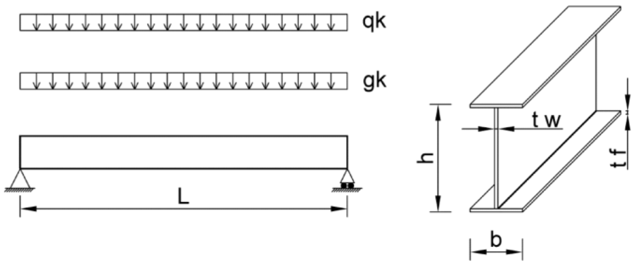
The beam is loaded by a uniformly-distributed dead load gk and a uniformly-distributed imposed load qk, as shown in Figure 1.
The civil engineer must evaluate the possible future levels of loading (self-weight, snow, wind), which the structure may be subjected to during its design life. Then, using hand calculations or computer methods, the loads acting on individual construction elements can be evaluated. The loads are used to calculate the shear forces, bending moments and deflections at critical sections along the construction elements. Finally, sufficient dimensions for the construction element can be defined.
4.1. Design Loads
The loads acting on a beam are divided into imposed and dead loads. For each type of loading there will be characteristic values and design values that must be estimated. In addition to this, the designer will have to determine the particular combination of loading that is likely to produce the most adverse effect on the structure in terms of shear forces, bending moments and deflections. The design loads are obtained by multiplying the characteristic loads by the partial safety factor for loads. However, before flexural members, such as beams, can be sized, the design bending moments and shear forces must be evaluated. Design shear forces and moments in beams are calculated using standard equations (Equations (21) and (22)). Having calculated the shear force and design bending moment, all that now remains to be done is to estimate the dimensions and strength of the beam required. Yield strength and section classification are used for the initial choice of the section. If the section is thick, i.e., has thick flanges and web, it can sustain the formation of a plastic hinge. On the other hand, a slender section, for example with thin flanges and web, will fail by local buckling before the yield stress can be reached.
Design action:
Design bending moment:
Design shear force:
Strength classification:
Section classification:
where:
and:
4.2. Resistance of Steel Cross-Sections
The structural design of steel beams primarily involves predicting the strength of their members. This requires the designer to imagine all of the ways in which each member may fail during its design life. Common modes of failure associated with beams are local buckling, shear, shear buckling, web bearing and buckling, lateral torsional buckling, bending and deflection.
4.2.1. Bending Moment
When shear force is absent or of a low value, the design value of the bending moment, MEd, at each section should satisfy the following:
where Mc,Rd is the design resistance for bending around one principal axis, taken as follows:
(a) the plastic design resistance moment of the gross section:
where Wpl is the plastic section modulus, for Class 1 and 2 sections only;
(b) the elastic design resistance moment of the gross section:
where Wel,min is the minimum elastic section modulus for Class 3 sections;
(c) the local buckling design resistance moment of the gross section:
where Weff,min is the minimum effective section modulus for Class 4 cross-sections only;
(d) the ultimate design resistance moment of the net section at bolt holes Mu,Rd, if this is less than the appropriate values above. In calculating this value, fastener holes in the compression zone do not need to be considered; they would need to be if they were oversized, slotted or filled by fasteners. In the tension zone, holes do not need to be considered, provided that:
4.2.2. Shear
The design value of the shear force VEd at each cross-section should satisfy the following:
where Vc,Rd is the design shear resistance. For the plastic design, Vc,Rd is taken as the design plastic shear resistance, Vpl,Rd, given by:
where Av is the shear area, which, for the rolled I and H sections, loaded parallel to the web, is:
where:
- b overall breadth
- r root radius
- tf flange thickness
- tw web thickness
- hw depth of the web
- η conservatively taken as 1.0
- A cross-sectional area
Fastener holes in the web do not have to be considered in shear verification. Shear buckling resistance for unstiffened webs must additionally be considered when:
For a stiffened web, shear buckling resistance will need to be considered when:
where kτ is the buckling factor for shear and is given by:
4.2.3. Resistance of Cross-Section-Bending and Shear
The plastic resistance moment of the section is reduced by the presence of shear force. When the design value of the shear force, VEd, exceeds 50 percent of the plastic shear design resistance, Vpl,Rd, the design resistance moment of the section, Mv,Rd, should be calculated using a reduced yield strength taken as:
Thus, for the rolled I and H sections, the reduced design resistance moment for the section around the major axis, My,v,Rd, will be given by:
4.2.4. Shear Buckling Resistance
As noted above, the shear buckling resistance of unstiffened beam webs has to be checked when:
The value of 1.0 for η for all steel grades up to and including S460 is recommended. For standard rolled beams and columns, this check is rarely necessary. However, as hw/tw is usually less than 72ε, it was not discussed in this section.
4.2.5. Flange-Induced Buckling
To prevent the possibility of the compression flange buckling in the plane of the web, Eurocode 3–5 [17] requires that the ratio hw/tw of the web should satisfy the following criterion:
where:
- Aw is the area of the web = (h−2∙tf)∙tw
- Afc is the area of the compression flange = b∙tf
- fyf is the yield strength of the compression flange
The factor k assumes the following values: plastic rotation utilized, i.e., Class 1 flanges: 0.3; plastic moment resistance utilized, i.e., Class 2 flanges: 0.4; elastic moment resistance utilized, i.e., Class 3 or Class 4 flanges: 0.55.
4.2.6. Resistance of the Web to Transverse Forces
Eurocode 3–5 [17] categorize between two types of forces applied through a flange to the web:
- (a)
- forces resisted by shear in the web (loading Types (a) and (c)).
- (b)
- forces transferred through the web directly to the other flange (loading Type (b)).
For loading Types (a) and (c), the web is likely to fail as a result of:
- (i)
- crushing of the web close to the flange accompanied by yielding of the flange; the combined effect is sometimes referred to as web crushing
- (ii)
- localized buckling and crushing of the web beneath the flange; the combined effect is sometimes referred to as web crippling.
For loading Type (b) the web is likely to fail as a result of:
- (i)
- web crushing
- (ii)
- buckling of the web over most of the depth of the member.
Provided that the compression flange is sufficiently restrained in the lateral direction, the design resistance of webs of beams under transverse forces can be determined in accordance with the recommendations in Eurocode 3 [17].
In Eurocode 3 [17], it is stated that the design resistance of webs to local buckling is given by:
where:
- fyw is the yield strength of the web
- tw is the thickness of the web
- γM1 is the partial safety factor = 1.0
- Leff is the effective length of the web that resists transverse forces = χFly, in which χF is the reduction factor due to local buckling.
- ly is the effective loaded length, appropriate to the length of the stiff bearing ss. As stated in Clause 6.3 of Eurocode 3–5 [17], ss should be taken as the distance over which the applied load is effectively distributed at a slope of 1:1, but ss ≤ hw.
Reduction factor, χF: The reduction factor χF is given by:
where:
in which:
Effective load length, ly: As stated in Clause 6.5 [17] for loading Types (a) and (b), the effective load length, ly, is given by:
where:
and if:
or if:
For loading Type (c), ly is taken as the smallest value obtained from Equations (52) and (53), as follows:
where:
4.3. Deflections
Several vertical deflections are defined in the Eurocode [18]. However, the National Annex to Eurocode 3 [17] recommends that verification of vertical deflections, δ, under unfactored imposed loads should be carried out. The designer is responsible for specifying appropriate limits of vertical deflections, which should be agreed upon with the client. However, like British Standard (BS) 5950 [19], the National Annex to Eurocode 3 [17] also recommends that verifications be made on vertical deflections, δ, under unfactored imposed loads. It suggests that in the absence of other limits, the recommendations in the Eurocode may be used.
The recommendations were examined and used for the building of the model and to predict the limits of vertical deflection. Two parameters with the biggest influence on the vertical deflection limits were considered. The influence of each parameter was determined on the basis of recommendations and engineering judgment. The comparison of different design codes (Eurocode, American Institute of Timber Construction (AITC) [20]) showed, that the deflection limits are very different. The study also suggests that deflection limits could be reconsidered in the future by the designers who have a prolonged or intense experience through practice.
4.3.1. ANFIS for the Development of the Constraint Function
A model to limit the vertical deflection based on recommendations was developed. The ANFIS model has two inputs: applied live load LL (kN/m2) and classification CLASS (-); and it has one output: LIMIT. The ANFIS-LIMIT model was proposed in order to calculate the deflection limits. MATLAB [16] and a Fuzzy Logic Toolbox were used as an interface for mathematical modeling and data handling.
One of the most important stages in the ANFIS technique is the collection of data. The training data were chosen based on the recommendations in AITC [20], Eurocode (Table 1), professional experience and past projects (Table 2). The classification used is separated into three groups. The first group is reserved for railway bridge stringers and beams used for commercial and institutional buildings with plaster ceilings. The second group is reserved for highway bridge stringers and beams used for commercial and institutional buildings without plaster ceilings. The third group is reserved for industrial roof beams.
The applied load (LL) and the classification system (CLASS) were taken as input parameters; whereas, the deflection limit (LIMIT) was considered as an output parameter. The training dataset (see Table 2) can be improved by adding additional recommendations and more past experience. These values can be assigned to the parameters and deflection limit. In this model, 33 evaluations were defined for a different applied live load and classification.
For the Sugeno fuzzy model [21], a rule set with i, i I, I = {1, 2} and fuzzy “if-then” rules were defined by Equations (55) and (56):
Rule 1: If LL is A1 and CLASS is B1, then:
Rule 2: If LL is A2 and CLASS is B2, then:
where are consequent parameters and LL and CLASS are input variables. The calculation procedure of the ANFIS models is as follows:
- the membership grade of the fuzzy set (Ai, Bi, Ci, Di) is calculated;
- the product of membership function for each rule is calculated;
- the ratio between the i-th rule’s firing strength and the sum of all rules’ firing strengths is calculated;
- the output of each rule is calculated; and
- the weighted average of each rule’s output is calculated.
The first membership grade of the fuzzy set (Ai, Bi, Ci, Di) is calculated with Equations (57) and (58):
where LL and CLASS are inputs to Gaussian membership functions, and the parameters cAi, cBi, σAi, σBi are premise parameters. In addition to this, the products between the membership functions for every rule are calculated; see Equations (59) and (60):
where w1 and w2 represent the firing strength of the each rule. The weighted average of each rules’ output is defined as the ratio between the i-th rule’s firing strength and the sum of all of the rule’s firing strengths; see Equation (61):
The output of each rule is finally determined as the sum of products between the weighted average of each rule’s output and the linear combination between input variables and consequent parameters:
For the model, the following values were evaluated: premise parameters, consequent parameters, firing strengths and weighted averages of rules outputs.
The structure of the model is shown in Figure 2. While the nodes on the left side represent the input data, the right node stands for the output. The model includes two inputs, the applied live load LL (kN/m2) and the classification CLASS (-), as well as a single output deflection limit LIMIT (-).
In a conventional fuzzy inference system, the number of rules is decided by the researcher/engineer who is familiar with the system to be modeled. There are no simple ways of determining in advance the minimum number of membership functions to achieve a desired performance level. In the present attempt, the number of membership functions assigned to each input variable was chosen empirically by examining the desired input-output data and by trial and error. For the deflection limit model, two membership functions were chosen for each input. Figure 2 shows the membership functions for LL and CLASS for the deflection model LIMIT. Note that all of the membership functions used were Gaussian membership functions, defined by Equations (57) and (58).
After the numbers of membership functions associated with each input were fixed, the initial values of premise parameters were set in such a way that membership functions were equally spaced along the operating range of each input variable. The LIMIT model contained two rules with two membership functions being assigned to each input variable. The total number of fitting parameters was 14, composed of eight premise parameters and six consequent parameters. These parameters were obtained by using a hybrid algorithm. MATLAB [16] was used as an interface for mathematical modeling. Premise and consequent parameters are presented in Table 3.
5. Fuzzy Optimization Model: Beam Implementation
In accordance with the exhaustive enumeration (EE) problem formulation, an EE optimization model for the optimization of a simply-supported beam (BEAM) was developed. Since the model BEAM is proposed to be used in the design of steel elements, all decisive design constraints were involved in the model. The model enables optimization of the system for various spans, loads and different material properties. For mathematical modeling and data input/output, a high level language, MATLAB [16], was used. The proposed optimization model includes input data, variables and the BEAM system’s weight objective function, which is subjected to the structure’s crisp and soft constraints; see Appendix A.
Choosing an I-beam from the list also identifies all of the design variables. This then becomes a single variable problem, the variable being the particular item from the list of beams.
The input data (constants) represent various design data for the optimization, i.e., constants/coefficients, which are involved in the objective function and (in) equality constraints. The design data are comprised of the span length L (m), the characteristic dead gk (kN/m) and imposed qk (kN/m) loads, the yield strength of the steel fy (MPa), the modulus of elasticity E (MPa), the density of the steel gam (kg/m3), bearings width ss (mm) and the allowable deflection of the beam lim (-). In addition to this, the data also include the coefficients involved in the design inequality constraints: safety factor for dead loads SFg (-), safety factor for imposed loads SFq (-), partial factor for resistance of cross-sections SFm0, partial factor for resistance of members to instability SFm1, modification factor k (-), non-dimensional slenderness lamflim (-) and the reduction factor for the relevant buckling curve ksiflim (-).
The objective variable f defines the weight of the steel beam. The aim of optimization is to find a steel beam with the minimum weight that satisfies all of the design constraints.
Design constraints that enable the ULS and SLS are satisfied by the following conditions:
- Condition 1, resistance of the cross-section to bending (ULS): verified by Equation (28), by which the design bending moment MEd (kNm) must not exceed the bending moment resistance MRd (kNm).
- Condition 2, resistance of the cross-section to shear (ULS): verified by Equation (33), by which the design shear force VEd (kN) must not exceed the shear resistance VRd (kNm).
- Condition 3, deflection (SLS) is considered: the calculated vertical deflection of the steel beam must be less than specified by the ANFIS-LIMIT model.
- Condition 4, resistance to flange-induced buckling (ULS): to prevent the possibility of the compression flange buckling in the plane of the web.
- Condition 5, Condition 6, Condition 7 and Condition 8, resistance of the web to transverse forces (ULS): to prevent the possibility of the local buckling of webs.
This is a single-variable problem, the variable being the particular item from the list of beams. In this case, there are no necessary geometrical constraints or side constraints. A complete enumeration can be performed on the selected beams from the stock list (see Appendix B), and the best beam can easily be identified.
In this example, the beam was used as a horizontal member. The objective was to design a minimum mass beam that would not fail, according to recommendations, under bending, shear and specified deflection. The length L of the beam was specified as 25 m. The steel beam was loaded by uniformly-distributed loading gk = 5 kN/m and qk = 15 kN/m, as shown below. Steel was chosen from the material of the beam. The modulus of elasticity of the steel was E = 210 GPa. The weight of the steel was ρ = 7850 kg/m3. The yield strength in tension was fy = 335 MPa. The specified applied load LL was 3 kN/m2 and used a classification of 1. A safety factor of 1.35 on the permanent load and 1.50 on the variable load were assumed. The results of an exhaustive enumeration computer code showed that the optimal section is HE 1000 × 393, with a weight of 9816.4 kg.
6. Conclusions
The article presents how recommendations can be implemented in a discrete optimization model. Good engineering judgment should be integrated into construction design; therefore, a mathematical model was developed based on engineering judgment and past experience. For this purpose, the theory of fuzzy sets was used. The advantages of the proposed fuzzy algorithm ANFIS are acknowledged and incorporated into the model based on the imprecision and fuzziness in the code-based design constraints. The comparison of different design codes showed that the deflection limits are very different and too liberal. The expert evaluations for the deflection limit are subjective; therefore, the data obtained from experts are expected to be vague, imprecise, incomplete or even contradictory. Additionally, the proposed ANFIS techniques include fuzzy clustering (FCM), which searches for patterns in data points [22]. The study also suggests that deflection limits could be reconsidered in the future by the experts who have a prolonged or intense experience through practice [23]. The advantages of using the exhaustive enumeration are reduced optimum weight values and obtaining a solution that is at a global optimum. The proposed computational model was used to find minimum weight solutions for simply-supported laterally-restrained beams. For selected design variables, an optimum steel section was found based on steel sections found on the market, according to the European beams tables. The computational model is based on advanced computational technologies, including fuzzy logic, neural networks and discrete optimization. It was developed to solve real-world problems that are of great interest to design engineers.
Author Contributions
The manuscript was written by both authors. The Assistant Professor Dr. Primož Jelušič developed the computer code. The Associate Professor Dr. Bojan Žlender developed the constraint function for limit deflection.
Conflicts of Interest
The authors declare no conflicts of interest.
Appendix A
Computer code for discrete optimization of fully laterally restrained beams with soft constraint ANFIS-LIMIT.
| % Optimization of Fully Laterally Restrained Beams with soft constrain | |
| % Simply supported steel beam | |
| %-------------------------------------------------- | |
| %%%%%%%%%%%%%%%%%%%%%%%%%%%%%%%%%%%%%%%%%%%%%%%%%%% | |
| % Discrete Optimization with soft constrain | |
| % Dr. P. Jelusic | |
| % See Text for Problem description | |
| % The Beam Properties are loaded from the file | |
| % BeamPropertiesEU.m | |
| %*************************************************** | |
| %%% | |
| clear | |
| clear global | |
| clc | |
| close | |
| format compact | |
| warning off | |
| %%% Run File %%%%%%%%% | |
| BeamPropertiesEU | |
| %%%%%%%%%%%%%%%%%%%%%%%% | |
| %%% monitor cpu time | |
| starttime = cputime; | |
| fprintf('\n********************************') | |
| fprintf('\nSimply supported steel beam (Enumeration)') | |
| fprintf | |
| % %****************************** | |
| % % Computer Code | |
| % %******************************* | |
| %Span, safety factors and loads | |
| L = 25; | % span (m) |
| SFg = 1.35; | % safety factor for dead load (-) |
| SFq = 1.50; | % safety factor for imposed load (-) |
| gk = 5; | % dead load(kN/m) |
| qk = 15; | % imposed load(kN/m) |
| ss = 100; | % bearings width (mm) |
| eta = 1; | % shear factor eta (-) |
| k = 0.3; | % factor k (-) |
| lamflim = 0.5; | % factor lamflim (-) |
| ksiflim = 1; | % factor ksiflim (-) |
| CLASS = 1; | % use classification (-) |
| LL = 3; | % Applied live load (kN/m2) |
| %ANFIS model coefficients | |
| sigA1 = 6.61768494044089; | |
| sigA2 = 7.47150990794045; | |
| sigB1 = 0.962309787332703; | |
| sigB2 = 0.979723951565027; | |
| cA1 = 2.90117735987428; | |
| cA2 = 2.08316049335067; | |
| cB1 = 1.62121248482762; | |
| cB2 = 1.27590144219536; | |
| a01 = -771.211045670957; | |
| a11 = 8.40911494744558; | |
| a21 = 172.024353054372; | |
| a02 = 1535.72815330126; | |
| a12 = -29.7774593495827; | |
| a22 = -158.884574516486; | |
| %Material properties | |
| fy = 355; | % yield strength (MPa) |
| E = 210000; | % modulus of elasticity (MPa) |
| SFmo = 1.00; | % safety factor for material bending (-) |
| SFm1 = 1.05; | % safety factor for elastic resistance deflection (-) |
| gam = 7850; | % density (kg/m3) |
| %%%Start Exhaustive Enumeration : | |
| fstar = inf; | |
| xstar = [inf inf inf inf]; | |
| gstar = [inf inf inf]; | |
| istar = 1; | |
| % % | |
| % | |
| fprintf('\n----------------------------') | |
| fprintf('\nFeasible Beams') | |
| fprintf('\n-----------------------------\n\n') | |
| for i = 1:length(RolledSteelBeamSI) | |
| x1 = RolledSteelBeamSI(i).D; | |
| x2 = RolledSteelBeamSI(i).B; | |
| x3 = RolledSteelBeamSI(i).tw; | |
| x4 = RolledSteelBeamSI(i).tf; | |
| %******************************* | |
| A = RolledSteelBeamSI(i).Area; | |
| D = RolledSteelBeamSI(i).D; | |
| B = RolledSteelBeamSI(i).B; | |
| tw = RolledSteelBeamSI(i).tw; | |
| tf = RolledSteelBeamSI(i).tf; | |
| Rr = RolledSteelBeamSI(i).Rr; | |
| dd = RolledSteelBeamSI(i).dd; | |
| Ix = RolledSteelBeamSI(i).Ix; | |
| Welx = RolledSteelBeamSI(i).Welx; | |
| Wplx = RolledSteelBeamSI(i).Wplx; | |
| %Design action. The reason for discrete optimization is to choose off-the-shelf I-beam which will keep the cost and production time down. Several mills provide information on standard rolling stock they manufacture. | |
| Fed = (SFg*(gk+A*gam*9.81/10000000) + SFq*qk)*L; | %design action (kN) |
| Med = Fed*L/8; | %design bending moment (kNm) |
| Ved = Fed/2; | %design shear force (kN) |
| %Section resistance | |
| Mrd = Wplx*fy/(SFmo*1000); | %moment resistance (kNm) |
| Av = A*100-2*B*tf + (tw + 2*Rr)*tf; | %shear area(mm2) |
| Vrd = Av*(fy/(3)^0.5)/(SFmo*1000); | %design shear resistance(kN) |
| %Deflection | |
| Mmax = (gk+qk)*L^2/8; | %maximum bending moment due to working load (kNm) |
| Mcrd = Welx*fy/(SFm1*1000); | %elastic resistance (kNm) |
| u = 5*qk*(L*1000)^4/(384*E*Ix*10000); | %deflection (mm) |
| %ANFIS calculation procedure | |
| A1ev = exp(-0.5*(((LL-cA1)/(sigA1))^2)); | |
| A2ev = exp(-0.5*(((LL-cA2)/(sigA2))^2)); | |
| B1ev = exp(-0.5*(((CLASS-cB1)/(sigB1))^2)); | |
| B2ev = exp(-0.5*(((CLASS-cB2)/(sigB2))^2)); | |
| w1 = A1ev*B1ev; | |
| w2 = A2ev*B2ev; | |
| w1n = w1/(w1+w2); | |
| w2n = w2/(w1+w2); | |
| fun1 = a01+a11*LL+a21*CLASS; | |
| fun2 = a02+a12*LL+a22*CLASS; | |
| nfun1 = w1n*fun1; | |
| nfun2 = w2n*fun2; | |
| lim = nfun1+nfun2; | |
| uult = L*1000/lim; | %permissible deflection (mm) |
| %Section classification | |
| eps = (235/fy)^0.5; | %factor eps (-) |
| c = (B-tw-2*Rr)/2; | %depth between fillets (mm) |
| hw = D-2*tf; | %depth between flanges (mm) |
| %Flange-induced buckling | |
| Aw = (D-2*tf)*tw; | %area of the web (mm2) |
| Afc = B*tf; | %area of the compression flange (mm2) |
| Fib = hw/tw; | %criteria ratio of flange-induced buckling(-) |
| Fibalw = k*(E/fy)*(Aw/Afc)^0.5; | %criteria ratio (-) |
| %Web buckling | |
| kf = 2+6*(ss/hw); | %buckling coefficient (-) |
| kfalw = 6; | %limit of buckling coefficient(-) |
| Fcr = (0.9*kf*E*tw^3)/hw; | %elastic critical buckling load(N) |
| m1 = fy*B/(fy*tw); | %coefficient m1(-) |
| m2 = 0.02*(hw/tf)^2; | %coefficient m2(-) |
| le = min(kf*E*tw^2/(2*fy*hw),ss); | %effective loaded length(mm) |
| ly = min(le+tf*(m1/2+(le/tf)^2+m2)^0.5,le + tf*(m1+m2)^0.5); | %(mm) |
| lamf = (ly*tw*fy/Fcr)^0.5; | %reduction factor lamf (-) |
| lamflim = 0.5; | %permissible reduction factor lamflim(-) |
| ksif = 0.5/lamf; | %reduction factor ksif(-) |
| leff = ksif*ly; | %effective length of web(mm) |
| Frdweb = fy*leff*tw/1000; | %design resistance of web(kN) |
| %Objective function | |
| f = gam*L*A/10000; | %weight of steel beam (kg) |
| %Constraints | |
| g1 = Med - Mrd; | %bending (kNm) |
| g2 = Ved - Vrd; | %shear (kN) |
| g3 = u - uult; | %deflection(mm) |
| g4 = Fib - Fibalw; | %flange-induced buckling (-) |
| g5 = kf - kfalw; | %web buckling constraint 1 (-) |
| g6 = lamflim - lamf; | %web buckling constraint 2 (-) |
| g7 = ksif - 1; | %web buckling constraint 3(-) |
| g8 = Ved - Frdweb; | %resistance of web constraint (kN) |
| %%% total constraint vector | |
| G = [g1 g2 g3 g4 g5 g6 g7 g8]; | |
| if (g1 <= 0) & (g2 <= 0) & (g3 <= 0) | |
| if (g4 <= 0) & (g5 <= 0) & (g6 <= 0) | |
| if (g7 <= 0) & (g8 <= 0) | |
| if (f <= fstar) | |
| xstar = [x1 x2 x3 x4]; | |
| fstar = f | |
| Gstar = G; | |
| istar = i | |
| end | |
| end | |
| end | |
| end | |
| end | |
| fprintf('\n******************************************') | |
| fprintf('\nOptimum Fully Laterally Restrained Beam') | |
| fprintf('\n******************************************\n\n') | |
| fprintf('Rolled Beam Designation : '),disp(RolledSteelBeamSI(istar).Name) | |
| fprintf('Depth(mm) Width(mm) Web Thickness(mm) Flange Thickness (mm)\n') | |
| fprintf('%8.5f %8.5f %8.5f %8.3f\n',xstar) | |
| fprintf('\nObjective Function(kg): '),disp(fstar) | |
| fprintf('\nConstraints\n') | |
| fprintf('---------------\n') | |
| fprintf('Bending Stress Constraint - g1 (kNm): '),disp(Gstar(1)) | |
| fprintf('Shear Stress Constraint - g2 (kN): '),disp(Gstar(2)) | |
| fprintf('Deflection Constraint - g3 (mm): '),disp(Gstar(3)) | |
| fprintf('flange-induced buckling - g4 (-): '),disp(Gstar(4)) | |
| fprintf('web buckling constraint 1 - g5 (-): '),disp(Gstar(5)) | |
| fprintf('web buckling constraint 2 - g6 (-): '),disp(Gstar(6)) | |
| fprintf('web buckling constraint 3 - g7 (-): '),disp(Gstar(7)) | |
| fprintf('resistance of web constraint - g8 (kN): '),disp(Gstar(8)) | |
| %%% print time | |
| totaltime = cputime - starttime; | |
| fprintf('\n\nTotal cpu time (s)= %7.4f \n\n',totaltime) | |
The companion file for the problem of fully-laterally-restrained beams is a file that contains beam properties for standard steel beams.
| % EE - Exhaustive Enumeration | |
| % For constrained optimization of fully laterally restrained beams | |
| % Dr. P. Jelusic | |
| % University of Maribor, Faculty of Civil Engineering | |
| %%%%%%%%%%%%%%%%%%%%%%%%%%%%%%%%%%%%%%%%%%%%%%%%%%%% | |
| %%% File UniversalbeamsEU.m | |
| %%%%%%%%%%%%%%%%%%%%%%%%%%%%%%%%%%%%%%%%%%%%%%%%%%%% | |
| % Discrete Variables | |
| %-------------------------------------------------- | |
| % See Text for Problem description | |
| %********************************************** | |
| %%% COMPANION FILE FOR PROBLEM Fully laterally restrained beams | |
| %%% This file contains Beam Properties for universal beams | |
| %%% beams in SI Units | |
| %********************************************** | |
| %%%%%%%%%%%%%%%%%%%%%%%%%%%%%%%%%%%%% | |
| %%% Define the section properties | |
| %%%%%%%%%%%%%%%%%%%%%%%%%%%%%%%%%%%% | |
| RolledSteelBeamSI(1).Name ='IPE AA 80'; | %beam identifier (-) |
| RolledSteelBeamSI(1).Area = 6.31; | %area (cm2) |
| RolledSteelBeamSI(1).D = 78; | %Depth of section (mm) |
| RolledSteelBeamSI(1).B = 46; | %width of section (mm) |
| RolledSteelBeamSI(1).tw = 3.2; | %web thickness (mm) |
| RolledSteelBeamSI(1).tf = 4.2; | %flange thickness (mm) |
| RolledSteelBeamSI(1).Rr = 5; | %root radius (mm) |
| RolledSteelBeamSI(1).dd = 59.6; | %depth between fillets(mm) |
| RolledSteelBeamSI(1).Ix = 64.1; | %second moment of area Ixx (cm4) |
| RolledSteelBeamSI(1).Welx = 16.4; | %elastic modulus Welx (cm3) |
| RolledSteelBeamSI(1).Wplx = 18.9; | %plastic modulus Wplx (cm3) |
| RolledSteelBeamSI(2) = struct('Name','IPE A 80','Area',6.38, ... | |
| 'D',78,'B',46,'tw',3.3,'tf',4.2, ... | |
| 'Rr',5,'dd',59.6,'Ix',64.4, ... | |
| 'Welx',16.5,'Wplx',19); | |
| RolledSteelBeamSI(3) = struct('Name','IPE 80','Area',7.64, ... | |
| 'D',80,'B',46,'tw',3.8,'tf',5.2, ... | |
| 'Rr',5,'dd',59.6,'Ix',80.1, ... | |
| 'Welx',20,'Wplx',23.2); | |
| RolledSteelBeamSI(75) = struct('Name','HE 1000 X 584','Area',743.7, ... | |
| 'D',1056,'B',314,'tw',36,'tf',64, ... | |
| 'Rr',30,'dd',868,'Ix',1246100, ... | |
| 'Welx',23600,'Wplx',28039); | |
| return; | |
The results are given in the following form:
| ****************************************** | |||
| Optimum Fully Laterally Restrained Beam | |||
| ****************************************** | |||
| Rolled Beam Designation : HE 1000 X 393 | |||
| Depth(mm) | Width(mm) | Web Thickness(mm) | Flange Thickness (mm) |
| 1016.00000 | 303.00000 | 24.40000 | 43.900 |
| Objective Function(kg): | 9.8164e+003 | ||
| Constraints | |||
| --------------- | |||
| Bending Stress Constraint | - g1 (kNm): | -3.8903e+003 | |
| Shear Stress Constraint | - g2 (kN): | -5.1282e+003 | |
| Deflection Constraint | - g3 (mm): | -12.9339 | |
| flange-induced buckling | - g4 (-): | -193.5248 | |
| web buckling constraint 1 | - g5 (-): | -3.3536 | |
| web buckling constraint 2 | - g6 (-): | -0.0742 | |
| web buckling constraint 3 | - g7 (-): | -0.1293 | |
| resistance of web constraint | - g8 (kN): | -1.8169e+003 | |
| Total cpu time (s)= | 0.2184 | ||
Appendix B

Table A1.
Dimensions and properties of steel beams (European beams).
| Designation | A | h | b | tw | tf | r | d | Iy | Wel.y | Wpl.y | Designation | A | h | b | tw | tf | r | d | Iy | Wel.y | Wpl.y |
|---|---|---|---|---|---|---|---|---|---|---|---|---|---|---|---|---|---|---|---|---|---|
| Serial Size | cm2 | mm | mm | mm | mm | mm | mm | cm4 | cm3 | cm3 | Serial Size | cm2 | mm | mm | mm | mm | mm | mm | cm4 | cm3 | cm3 |
| IPE AA 80 | 6.31 | 78 | 46 | 3.2 | 4.2 | 5 | 59.6 | 64.1 | 16.4 | 18.9 | IPE O 360 | 84.1 | 364 | 172 | 9.2 | 14.7 | 18 | 298.6 | 19,050 | 1047 | 1186 |
| IPE A 80 | 6.38 | 78 | 46 | 3.3 | 4.2 | 5 | 59.6 | 64.4 | 16.5 | 19 | IPE A 400 | 73.1 | 397 | 180 | 7 | 12 | 21 | 331 | 20,290 | 1022 | 1144 |
| IPE 80 | 7.64 | 80 | 46 | 3.8 | 5.2 | 5 | 59.6 | 80.1 | 20 | 23.2 | IPE 400 | 84.5 | 400 | 180 | 8.6 | 13.5 | 21 | 331 | 23,130 | 1160 | 1307 |
| IPE AA 100 | 8.56 | 97.6 | 55 | 3.6 | 4.5 | 7 | 74.6 | 136 | 27.9 | 31.9 | IPE O 400 | 96.4 | 404 | 182 | 9.7 | 15.5 | 21 | 331 | 26,750 | 1324 | 1502 |
| IPE A 100 | 8.8 | 98 | 55 | 3.6 | 4.7 | 7 | 74.6 | 141 | 28.8 | 33 | IPE A 450 | 85.6 | 447 | 190 | 7.6 | 13.1 | 21 | 378.8 | 29,760 | 1331 | 1494 |
| IPE 100 | 10.3 | 100 | 55 | 4.1 | 5.7 | 7 | 74.6 | 171 | 34.2 | 39.4 | IPE 450 | 98.8 | 450 | 190 | 9.4 | 14.6 | 21 | 378.8 | 33,740 | 1500 | 1702 |
| IPE AA 120 | 10.7 | 117 | 64 | 3.8 | 4.8 | 7 | 93.4 | 244 | 41.7 | 47.6 | IPE O 450 | 118 | 456 | 192 | 11 | 17.6 | 21 | 378.8 | 40,920 | 1795 | 2046 |
| IPE A 120 | 11 | 117.6 | 64 | 3.8 | 5.1 | 7 | 93.4 | 257 | 43.8 | 49.9 | IPE A 500 | 101 | 497 | 200 | 8.4 | 14.5 | 21 | 426 | 42,930 | 1728 | 1946 |
| IPE 120 | 13.2 | 120 | 64 | 4.4 | 6.3 | 7 | 93.4 | 318 | 53 | 60.7 | IPE 500 | 116 | 500 | 200 | 10.2 | 16 | 21 | 426 | 48,200 | 1930 | 2194 |
| IPE AA 140 | 12.8 | 136.6 | 73 | 3.8 | 5.2 | 7 | 112.2 | 407 | 59.7 | 67.6 | IPE O 500 | 137 | 506 | 202 | 12 | 19 | 21 | 426 | 57,780 | 2284 | 2613 |
| IPE A 140 | 13.4 | 137.4 | 73 | 3.8 | 5.6 | 7 | 112.2 | 435 | 63.3 | 71.6 | IPE A 550 | 117 | 547 | 210 | 9 | 15.7 | 24 | 467.6 | 59,980 | 2193 | 2475 |
| IPE 140 | 16.4 | 140 | 73 | 4.7 | 6.9 | 7 | 112.2 | 541 | 77.3 | 88.3 | IPE 550 | 134 | 550 | 210 | 11.1 | 17.2 | 24 | 467.6 | 67,120 | 2440 | 2787 |
| IPE AA 160 | 15.4 | 156.4 | 82 | 4 | 5.6 | 7 | 131.2 | 646 | 82.6 | 93.3 | IPE O 550 | 156 | 556 | 212 | 12.7 | 20.2 | 24 | 467.6 | 79,160 | 2847 | 3263 |
| IPE A 160 | 16.2 | 157 | 82 | 4 | 5.9 | 9 | 127.2 | 689 | 87.8 | 99.1 | IPE A 600 | 137 | 597 | 220 | 9.8 | 17.5 | 24 | 514 | 82,920 | 2778 | 3141 |
| IPE 160 | 20.1 | 160 | 82 | 5 | 7.4 | 9 | 127.2 | 869 | 109 | 124 | IPE 600 | 156 | 600 | 220 | 12 | 19 | 24 | 514 | 92,080 | 3070 | 3512 |
| IPE AA 180 | 19 | 176.4 | 91 | 4.3 | 6.2 | 9 | 146 | 1020 | 116 | 131 | IPE O 600 | 197 | 610 | 224 | 15 | 24 | 24 | 514 | 118,300 | 3879 | 4471 |
| IPE A 180 | 19.6 | 177 | 91 | 4.3 | 6.5 | 9 | 146 | 1063 | 120 | 135 | IPE 750 × 134 | 171 | 750 | 264 | 12 | 15.5 | 17 | 685 | 150,700 | 4018 | 4644 |
| IPE 180 | 23.9 | 180 | 91 | 5.3 | 8 | 9 | 146 | 1317 | 146 | 166 | IPE 750 × 147 | 188 | 753 | 265 | 13.2 | 17 | 17 | 685 | 166,100 | 4411 | 5110 |
| IPE O 180 | 27.1 | 182 | 92 | 6 | 9 | 9 | 146 | 1505 | 165 | 189 | IPE 750 × 173 | 221 | 762 | 267 | 14.4 | 21.6 | 17 | 685 | 205,800 | 5402 | 6218 |
| IPE AA 200 | 22.9 | 196.4 | 100 | 4.5 | 6.7 | 12 | 159 | 1533 | 156 | 176 | IPE 750 × 196 | 251 | 770 | 268 | 15.6 | 25.4 | 17 | 685 | 240,300 | 6241 | 7174 |
| IPE A 200 | 23.5 | 197 | 100 | 4.5 | 7 | 12 | 159 | 1591 | 162 | 182 | HE 100 A | 21.2 | 96 | 100 | 5 | 8 | 12 | 56 | 349.2 | 72.76 | 83.01 |
| IPE 200 | 28.5 | 200 | 100 | 5.6 | 8.5 | 12 | 159 | 1943 | 194 | 221 | HE 100 B | 26 | 100 | 100 | 6 | 10 | 12 | 56 | 449.5 | 89.91 | 104.2 |
| IPE O 200 | 32 | 202 | 102 | 6.2 | 9.5 | 12 | 159 | 2211 | 219 | 249 | HE 120 A | 25.3 | 114 | 120 | 5 | 8 | 12 | 74 | 606.2 | 106.3 | 119.5 |
| IPE AA 220 | 27 | 216.4 | 110 | 4.7 | 7.4 | 12 | 177.6 | 2219 | 205 | 230 | HE 120 B | 34 | 120 | 120 | 6.5 | 11 | 12 | 74 | 864.4 | 144.1 | 165.2 |
| IPE A 220 | 28.3 | 217 | 110 | 5 | 7.7 | 12 | 177.6 | 2317 | 214 | 240 | HE 140 A | 31.4 | 133 | 140 | 5.5 | 8.5 | 12 | 92 | 1033 | 155.4 | 173.5 |
| IPE 220 | 33.4 | 220 | 110 | 5.9 | 9.2 | 12 | 177.6 | 2772 | 252 | 285 | HE 140 B | 43 | 140 | 140 | 7 | 12 | 12 | 92 | 1509 | 215.6 | 245.4 |
| IPE O 220 | 37.4 | 222 | 112 | 6.6 | 10.2 | 12 | 177.6 | 3134 | 282 | 321 | HE 300 A | 112.5 | 290 | 300 | 8.5 | 14 | 27 | 208 | 18,260 | 1260 | 1383 |
| IPE AA 240 | 31.7 | 236.4 | 120 | 4.8 | 8 | 15 | 190.4 | 3154 | 267 | 298 | HE 300 B | 149.1 | 300 | 300 | 11 | 19 | 27 | 208 | 25,170 | 1678 | 1869 |
| IPE A 240 | 33.3 | 237 | 120 | 5.2 | 8.3 | 15 | 190.4 | 3290 | 278 | 312 | HE 300 M | 303.1 | 340 | 310 | 21 | 39 | 27 | 208 | 59,200 | 3482 | 4078 |
| IPE 240 | 39.1 | 240 | 120 | 6.2 | 9.8 | 15 | 190.4 | 3892 | 324 | 367 | HE 700 A | 260.5 | 690 | 300 | 14.5 | 27 | 27 | 582 | 215,300 | 6241 | 7032 |
| IPE O 240 | 43.7 | 242 | 122 | 7 | 10.8 | 15 | 190.4 | 4369 | 361 | 410 | HE 700 B | 306.4 | 700 | 300 | 17 | 32 | 27 | 582 | 256,900 | 7340 | 8327 |
| IPE A 270 | 39.2 | 267 | 135 | 5.5 | 8.7 | 15 | 219.6 | 4917 | 368 | 413 | HE 800 AA | 218.5 | 770 | 300 | 14 | 18 | 30 | 674 | 208,900 | 5426 | 6225 |
| IPE 270 | 45.9 | 270 | 135 | 6.6 | 10.2 | 15 | 219.6 | 5790 | 429 | 484 | HE 800 A | 285.8 | 790 | 300 | 15 | 28 | 30 | 674 | 303,400 | 7682 | 8699 |
| IPE O 270 | 53.8 | 274 | 136 | 7.5 | 12.2 | 15 | 219.6 | 6947 | 507 | 575 | HE 900 AA | 252.2 | 870 | 300 | 15 | 20 | 30 | 770 | 301,100 | 6923 | 7999 |
| IPE A 300 | 46.5 | 297 | 150 | 6.1 | 9.2 | 15 | 248.6 | 7173 | 483 | 542 | HE 900 A | 320.5 | 890 | 300 | 16 | 30 | 30 | 770 | 422,100 | 9485 | 10,810 |
| IPE 300 | 53.8 | 300 | 150 | 7.1 | 10.7 | 15 | 248.6 | 8356 | 557 | 628 | HE 900 × 466 | 593.7 | 938 | 312 | 30 | 54 | 30 | 770 | 814,900 | 17,380 | 20,380 |
| IPE O 300 | 62.8 | 304 | 152 | 8 | 12.7 | 15 | 248.6 | 9994 | 658 | 744 | HE 1000 AA | 282.2 | 970 | 300 | 16 | 21 | 30 | 868 | 406,500 | 8380 | 9777 |
| IPE A 330 | 54.7 | 327 | 160 | 6.5 | 10 | 18 | 271 | 10,230 | 626 | 702 | HE 1000 A | 346.8 | 990 | 300 | 16.5 | 31 | 30 | 868 | 553,800 | 11,190 | 12,820 |
| IPE 330 | 62.6 | 330 | 160 | 7.5 | 11.5 | 18 | 271 | 11,770 | 713 | 804 | HE 1000 × 393 | 500.2 | 1016 | 303 | 24.4 | 43.9 | 30 | 868 | 807,700 | 15,900 | 18,540 |
| IPE O 330 | 72.6 | 334 | 162 | 8.5 | 13.5 | 18 | 271 | 13,910 | 833 | 943 | HE 1000 × 415 | 528.7 | 1020 | 304 | 26 | 46 | 30 | 868 | 853,100 | 16,728 | 19,571 |
| IPE A 360 | 64 | 357.6 | 170 | 6.6 | 11.5 | 18 | 298.6 | 14,520 | 812 | 907 | HE 1000 × 438 | 556 | 1026 | 305 | 26.9 | 49 | 30 | 868 | 909,200 | 17,720 | 20,750 |
| IPE 360 | 72.7 | 360 | 170 | 8 | 12.7 | 18 | 298.6 | 16,270 | 904 | 1019 | HE 1000 × 494 | 629.1 | 1036 | 309 | 31 | 54 | 30 | 868 | 1,028,000 | 19,845 | 23,413 |
References
- Adeli, H.; Sarma, K.C. Cost Optimization of Structures: Fuzzy Logic, Genetic Algorithms, and Parallel Computing; John Wiley & Sons: Chichester, UK, 2006. [Google Scholar]
- Adeli, H. Knowledge Engineering: Fundamentals; McGraw-Hill: New York, NY, USA, 1990. [Google Scholar]
- Soh, C.K.; Yang, J. Fuzzy controlled genetic algorithm search for shape optimization. J. Comput. Civ. Eng. 1996, 10, 143–150. [Google Scholar] [CrossRef]
- Smith, A.E.; Tate, D.M. Genetic optimization using a penalty function. In Proceedings of the Fifth International Conference on Genetic Algorithms, Champaign, IL, USA, 17–21 July 1993; pp. 499–505. [Google Scholar]
- Kim, J.H.; Myung, H. Evolutionary programming techniques for constrained optimization problems. IEEE Trans. Evolut. Comput. 1997, 1, 129–140. [Google Scholar]
- Adeli, H.; Cheng, N.T. Augmented Lagrangian genetic algorithm for structural optimization. J. Aerosp. Eng. 1994, 7, 104–118. [Google Scholar] [CrossRef]
- Adeli, H.; Park, H.S. Optimization of space structures by neural dynamics model. Neural Netw. 1995, 8, 769–781. [Google Scholar] [CrossRef]
- Adeli, H.; Park, H.S. Neurocomputing for Design Automation; CRC Press: Boca Raton, FL, USA, 1998. [Google Scholar]
- Wang, G.; Wang, W. Fuzzy optimum design of aseismic structures. Earthq. Eng. Struct. Dyn. 1985, 13, 827–837. [Google Scholar]
- Rao, S.S. Description and optimum design of fuzzy mechanical systems. J. Mech. Transm. Autom. Des. 1987, 109, 126–132. [Google Scholar] [CrossRef]
- Yeh, Y.; Hsu, D. Structural optimization with fuzzy parameters. Comput. Struct. 1990, 37, 917–924. [Google Scholar]
- Jelusic, P. Soil compaction optimization with soft constrain. J. Intell. Fuzzy Syst. 2015, 29, 955–962. [Google Scholar] [CrossRef]
- Bellman, R.E.; Zadeh, L.A. Decision-making in a fuzzy environment. Manag. Sci. 1970, 17, B141–B164. [Google Scholar] [CrossRef]
- Zimmermann, H.J. Fuzzy programming and linear programming with several objective functions. Fuzzy Sets Syst. 1978, 1, 45–55. [Google Scholar] [CrossRef]
- Jang, J.S.R. ANFIS: Adaptive-network-based fuzzy inference system. IEEE Trans. Syst. Man Cybern. 1993, 23, 665–685. [Google Scholar]
- MathWorks. MATLAB Function Reference; The MathWorks, Inc.: Natick, MA, USA, 2010. [Google Scholar]
- European Committee for Standardization. Eurocode 3: Design of Steel Structures; EN 1993; CEN: Brussels, Belgium, 2002. [Google Scholar]
- European Committee for Standardization. Eurocode: Basis of Structural Design; EN 1990; CEN: Brussels, Belgium, 2002. [Google Scholar]
- British Standard. Structural Use of Steelwork in Building—Part 1: Code of Practice for Design—Rolled and Welded Sections; BS 5950-1; BSI: London, UK, 2000. [Google Scholar]
- American Institute of Timber Construction. Timber Construction Manual, 5th ed.; John Wiley and Sons: Hoboken, NJ, USA, 2005. [Google Scholar]
- Sugeno, M. Industrial Applications of Fuzzy Control; Elsevier Science Pub. Co: New York, NY, USA, 1985. [Google Scholar]
- Jelušič, P.; Žlender, B. Soil-nail wall stability analysis using ANFIS. Acta Geotech. Slov. 2013, 10, 61–73. [Google Scholar]
- Jelušič, P.; Žlender, B. An adaptive network fuzzy inference system approach for site investigation. Geotech. Test. J. 2014, 37, 400–411. [Google Scholar] [CrossRef]
Figure 1.
Simply-supported beam and steel section.

Figure 2.
Fuzzy inference system implemented within the framework of adaptive networks ANFIS-LIMIT.
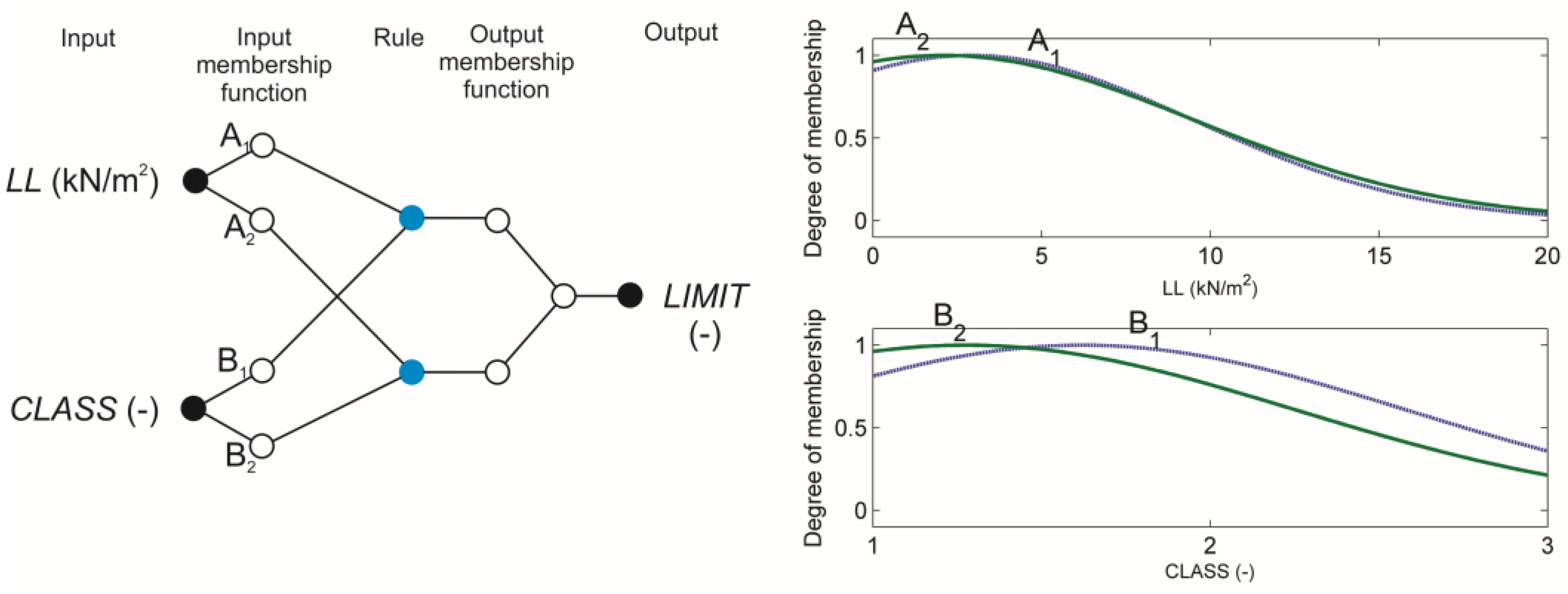
Table 1.
Deflection limit according to the recommendations.
| Use Classification | Deflection Limit |
|---|---|
| Roof beams (industrial) | L/180 |
| Roof beams (commercial and institutional without plaster ceiling) | L/240 |
| Roof beams (commercial and institutional with plaster ceiling) | L/360 |
| Floor beams (ordinary usage) | L/360 |
| Highway bridge stringers | L/200 to L/300 |
| Railway bridge stringers | L/300 to L/400 |
| LL < 2.5 kN/m2 | L/480 |
| 2.5 kN/m2 < LL < 4.0 kN/m2 | L/420 |
| LL > 4.0 kN/m2 | L/360 |
Table 2.
Training data for the ANFIS-LIMIT model.
| Inputs | Output | |
|---|---|---|
| Applied Live Load LL | Classification | Deflection Limit |
| (kN/m2) | CLASS * | LIMIT |
| 20 | 1 | 360 |
| 10 | 1 | 360 |
| 4 | 1 | 360 |
| 3.5 | 1 | 420 |
| 3 | 1 | 420 |
| 2.5 | 1 | 480 |
| 2 | 1 | 480 |
| 1.5 | 1 | 480 |
| 1 | 1 | 480 |
| 0.5 | 1 | 480 |
| 0 | 1 | 480 |
| 20 | 2 | 240 |
| 10 | 2 | 240 |
| 4 | 2 | 240 |
| 3.5 | 2 | 280 |
| 3 | 2 | 280 |
| 2.5 | 2 | 320 |
| 2 | 2 | 320 |
| 1.5 | 2 | 320 |
| 1 | 2 | 320 |
| 0.5 | 2 | 320 |
| 0 | 2 | 320 |
| 20 | 3 | 180 |
| 10 | 3 | 180 |
| 4 | 3 | 180 |
| 3.5 | 3 | 210 |
| 3 | 3 | 210 |
| 2.5 | 3 | 240 |
| 2 | 3 | 240 |
| 1.5 | 3 | 240 |
| 1 | 3 | 240 |
| 0.5 | 3 | 240 |
| 0 | 3 | 240 |
* 1, Railway bridge stringers, beams used for commercial and institutional buildings with plaster ceiling; 2, highway bridge stringers and beams used for commercial and institutional buildings without plaster ceiling; 3, industrial roof beams.
Table 3.
Premise and consequent parameters of the ANFIS-LIMIT model.
| Membership Function | Premise Parameters | Consequent Parameters | ||
|---|---|---|---|---|
| i | σi | ci | - | |
| A1 | 6.61768494044089 | 2.90117735987428 | a01 | −771.211045670957 |
| A2 | 7.47150990794045 | 2.08316049335067 | a11 | 8.40911494744558 |
| B1 | 0.962309787332703 | 1.62121248482762 | a21 | 172.024353054372 |
| B2 | 0.979723951565027 | 1.27590144219536 | a02 | 1535.72815330126 |
| - | - | - | a12 | −29.7774593495827 |
| - | - | - | a22 | −158.884574516486 |
© 2017 by the authors. Licensee MDPI, Basel, Switzerland. This article is an open access article distributed under the terms and conditions of the Creative Commons Attribution (CC BY) license (http://creativecommons.org/licenses/by/4.0/).
Share and Cite
MDPI and ACS Style
Jelušič, P.; Žlender, B. Discrete Optimization with Fuzzy Constraints. Symmetry 2017, 9, 87. https://doi.org/10.3390/sym9060087
AMA Style
Jelušič P, Žlender B. Discrete Optimization with Fuzzy Constraints. Symmetry. 2017; 9(6):87. https://doi.org/10.3390/sym9060087
Chicago/Turabian StyleJelušič, Primož, and Bojan Žlender. 2017. "Discrete Optimization with Fuzzy Constraints" Symmetry 9, no. 6: 87. https://doi.org/10.3390/sym9060087
Note that from the first issue of 2016, this journal uses article numbers instead of page numbers. See further details here.