
Focus Assessment Method of Gaze Tracking Camera Based on ε-Support Vector Regression

Division of Electronics and Electrical Engineering, Dongguk University, 30 Pildong-ro 1-gil, Jung-gu, Seoul 100-715, Korea
*
Author to whom correspondence should be addressed.
Symmetry 2017, 9(6), 86; https://doi.org/10.3390/sym9060086
Submission received: 16 April 2017
/
Revised: 6 June 2017
/
Accepted: 8 June 2017
/
Published: 14 June 2017
Abstract
:In order to capture an eye image of high quality in a gaze-tracking camera, an auto-focusing mechanism is used, which requires accurate focus assessment. Although there has been previous research on focus assessment in the spatial or wavelet domains, there are few previous studies that combine all of the methods of spatial and wavelet domains. Since all of the previous focus assessments in the spatial or wavelet domain methods have disadvantages, such as being affected by illumination variation, etc., we propose a new focus assessment method by combining the spatial and wavelet domain methods for the gaze-tracking camera. This research is novel in the following three ways, in comparison with the previous methods. First, the proposed focus assessment method combines the advantages of spatial and wavelet domain methods by using ε-support vector regression (SVR) with a symmetrical Gaussian radial basis function (RBF) kernel. In order to prevent the focus score from being affected by a change in image brightness, both linear and nonlinear normalizations are adopted in the focus score calculation. Second, based on the camera optics, we mathematically prove the reason for the increase in the focus score in the case of daytime images or a brighter illuminator compared to nighttime images or a darker illuminator. Third, we propose a new criterion to compare the accuracies of the focus measurement methods. This criterion is based on the ratio of relative overlapping amount (standard deviation of focus score) between two adjacent positions along the Z-axis to the entire range of focus score variety between these two points. Experimental results showed that the proposed method outperforms other methods.
1. Introduction
1.1. Motivation
Gaze tracking is the technology to calculate the position that a user is looking at based on captured eye images [1,2,3,4,5,6,7], and it can be used in various fields of human computer interface, interface for the disabled and monitoring of driver’s status. The eye image of high quality is required to achieve a high accuracy of gaze detection, and an accurate auto-focusing method is required for this purpose. Without the auto-focusing method, the camera with a single focal length (not a variable focal length) having a large depth of field (DOF) can be considered as an alternative. DOF is the Z distance range from the camera lens to the object, and a focused image can be usually captured within the DOF. Using a lens with a small DOF, the input eye image is easily (optically) blurred, and the consequent detection error of pupil and corneal specular reflection (SR) is increased, which increases the final gaze detection error. In order to increase the DOF of the lens, the f-number of the lens should be increased. Further, the f-number is inversely proportional to the diameter of the lens (lens aperture) [8]. Therefore, in order to obtain a large f-number, a lens with a small diameter should be used, which causes the input image to be too dark for the regions of pupil and corneal SR to be detected correctly. To overcome the problem of the limitation of DOF, an accurate auto-focusing system is considered for the gaze-tracking camera. Auto-focusing enables the camera lens to focus on an object based on the score measured by the focus assessment method. Therefore, accurate focus assessment is a prerequisite for auto-focusing.
In this paper, we suggest a new method of focus assessment using ε-support vector regression (ε-SVR). In our method, four focus scores calculated by four focus measurements—Daugman’s convolution kernel [9], Kang’s convolution kernel [10], Daubechies wavelet transform [11] and Haar wavelet transform—are used as the inputs of ε-SVR. Using the four focus measures of the same image, the trained ε-SVR can produce a more accurate focus score as the output.
1.2. Related Works
Previous research about focus measurement can be classified into two categories: spatial domain-based methods [9,10,12,13,14,15] and wavelet domain-based methods [11,16,17]. In the spatial domain, Daugman proposed an 8 × 8 convolution kernel for measuring the focus value [9]. Since Daugman’s kernel passes the low frequency components, the focus measurement is affected by a change in image brightness. Kang et al. [10] proposed a 5 × 5 convolution kernel. Compared to Daugman’s kernel, Kang’s convolution kernel showed a more distinctive change in the focus score according to the image blurring. However, by using the smaller mask of 5 × 5 compared to Daugman’s 8 × 8 mask, its performance can be affected by the local high frequency components of iris patterns. Wan et al. [12] proposed another spatial domain method based on the Laplacian of Gaussian (LoG) operator. The processed image by the Laplacian operator based on a second derivative is usually sensitive to noise. To overcome this problem, a Gaussian smoothing filter is used before applying the Laplacian. Wan et al. suggested a method using two commonly-used 3 × 3 kernels to simplify the computation. Similar to previous research [9,10], they used an image that includes only the eye area without the eyebrow regions, since they assumed that the input image in a conventional iris recognition camera includes only the eye area without eyebrows. However, a gaze-tracking camera can include a wider area including the eyes and the eyebrows, as shown in Figure 1, and the eyebrow region can cause an incorrect increment of the focus score. In other words, even if the eye region is not focused, the focus score of the input image can be high, owing to thick eyebrows.
Alternatively, Grabowski et al. [13] suggested a method using entropy as the score of the focus measurement. In their research, the focus condition of an input image was considered in terms of the quantity of information that can be calculated by entropy. Accordingly, the more focused the input image, the higher the entropy value. However, the existence of eyebrows in the captured image can affect the focus scores calculated using entropy.
Furthermore, Zhang et al. [14] proposed a region-based fusion algorithm of multi-focus images by using the quality assessment in spatial domain. In addition, the genetic algorithm based on the feature and pixel-level fusion was used in this research. However, they have experimented with the images of the general scene (not eye or iris images), and their algorithm is difficult to apply to eye images owing to the different traits of eye images such as eyebrows, eyelashes and iris patterns. Wei et al. [15] proposed a 5 × 5 mask for calculating the focus score of an iris image, but similar to previous research [9,10], they used an image that includes only the iris area without the eyebrow regions. The existence of eyebrows in the captured image can affect the focus scores calculated using their method.
In the wavelet domain, Kautsky et al. [16] suggested a measure of image focus based on the wavelet transform of an image. In this research, the measure of image focus is defined as the ratio of high-pass band to low-pass band norms. In another research work, Jang et al. proposed a method combining the wavelet transform method and the support vector machine (SVM) [11]. The results showed that their method could overcome the disadvantages of Kautsky’s work. However, it is not easy to determine the passing band in the frequency domain by selecting the type of wavelet kernel and the decomposition level. In addition, the focus score is more significantly affected by the change in brightness of the input image than in the spatial domain.
A blind assessment method of image blur based on Haar wavelet transform (HWT) was proposed by Bachoo [17]. In this research, two first derivatives of the images by a 3 × 3 Sobel operator were used in HWT to collect the sum of energies of the high-low (HL) and low-high (LH) sub-bands of each scale. The blur amount was defined as the ratio of the aforementioned sum to the total energy of the images. However, they measured the accuracies only with the images of the general scene (not eye or iris images).
Although there has been previous research on focus assessment in the spatial or wavelet domains, there are few previous studies that combined all of the methods of the spatial and wavelet domains. Since all of the previous focus assessments in the spatial or wavelet domain methods have disadvantages, such as being affected by illumination variation, etc., we propose a new focus assessment method by combining the spatial and wavelet domain methods based on ε-SVR.
Table 1 shows the summarized comparison of the previous and proposed focus assessment methods.
The structure of this paper is as follows. In Section 2, we present an overview of our gaze-tracking system, the overall flowchart of the proposed focus assessment method, the details of four individual methods of focus measurement and their combination using ε-SVR. Section 3 illustrates our experimental results, and finally, the conclusion of our research is presented in Section 4.
2. Proposed Method
2.1. Overview of the Proposed Method
Figure 1 shows the proposed gaze-tracking system for an intelligent TV interface. The capturing device, as shown in Figure 1, includes two panning and tilting and focusing functional cameras: a wide-view camera for face and eye detection and a narrow-view camera for gaze tracking. Therefore, the captured eye images can be used for the gaze position calculation using the detected pupil center and the four detected SRs, each caused by a near-infrared (NIR) illuminator at one of the four corners of the TV monitor. The gaze-tracking camera includes a long focal length lens, whose DOF is small, which causes the input eye image to be blurred easily. An accurate focus measurement method is required to overcome the limited DOF of the lens. Hence, the proposed method that combines four focus assessments is applied. The proposed method is shown in a flowchart in Figure 2.
Since both the spatial and wavelet domain methods are sensitive to brightness change, we perform linear normalization in order to normalize the brightness of the input images. Subsequently, the four individual focus measurements—Daugman’s convolution kernel [9], Kang’s convolution kernel [10], Daubechies wavelet transform [11] and Haar wavelet transform [18]—are used to obtain four separate focus levels, which are nonlinear normalized to obtain a range from 0 to 1.
In terms of computing running averages and differences by using scalar products with wavelets and scaling signals, the Haar wavelet transform is defined in the same way as the Daubechies wavelet transform. The only difference of these two transforms is how the wavelets and the scaling signals are defined. In detail, in the case of the Daubechies wavelet transform, the wavelets and scaling signals have slightly longer supports, i.e., they generate the values of averages and differences with more values from the signal than the Haar wavelet transform. However, this difference can cause improvement in the capabilities of wavelet transform. The examples of the shape of wavelet and scaling functions of the Daubechies wavelet transform can be referred to [19], whereas those of the Haar wavelet transform can be referred to [19]. Subsequently, ε-SVR is applied to combine the four measurements in order to obtain a unique focus score, which is more accurate than the four focus scores.
2.2. Linear Normalization of Image Brightness Based on Mathematical Analyses
In spatial domain methods, the masks work as filters to collect the high frequency energy components of the images. The convolution value increases with an increase in the image brightness. Consequently, the calculated focus score can be high when the brightness is high, even if the actual focus level is very low. Thus, the focus score graph of dark images is usually lower than that of bright images. In wavelet domain methods, the phase and amplitude of the wavelet cannot be separated in the transform process [20]. The amplitude is related to the image brightness. For example, if the image becomes too dark, the high frequency components of the image decrease, whereas the low frequency components increase, resulting in a low response of the focus measure. These phenomena, caused by image brightness variation in the spatial and wavelet domains, are shown in Figure 3 and Figure 4, respectively.
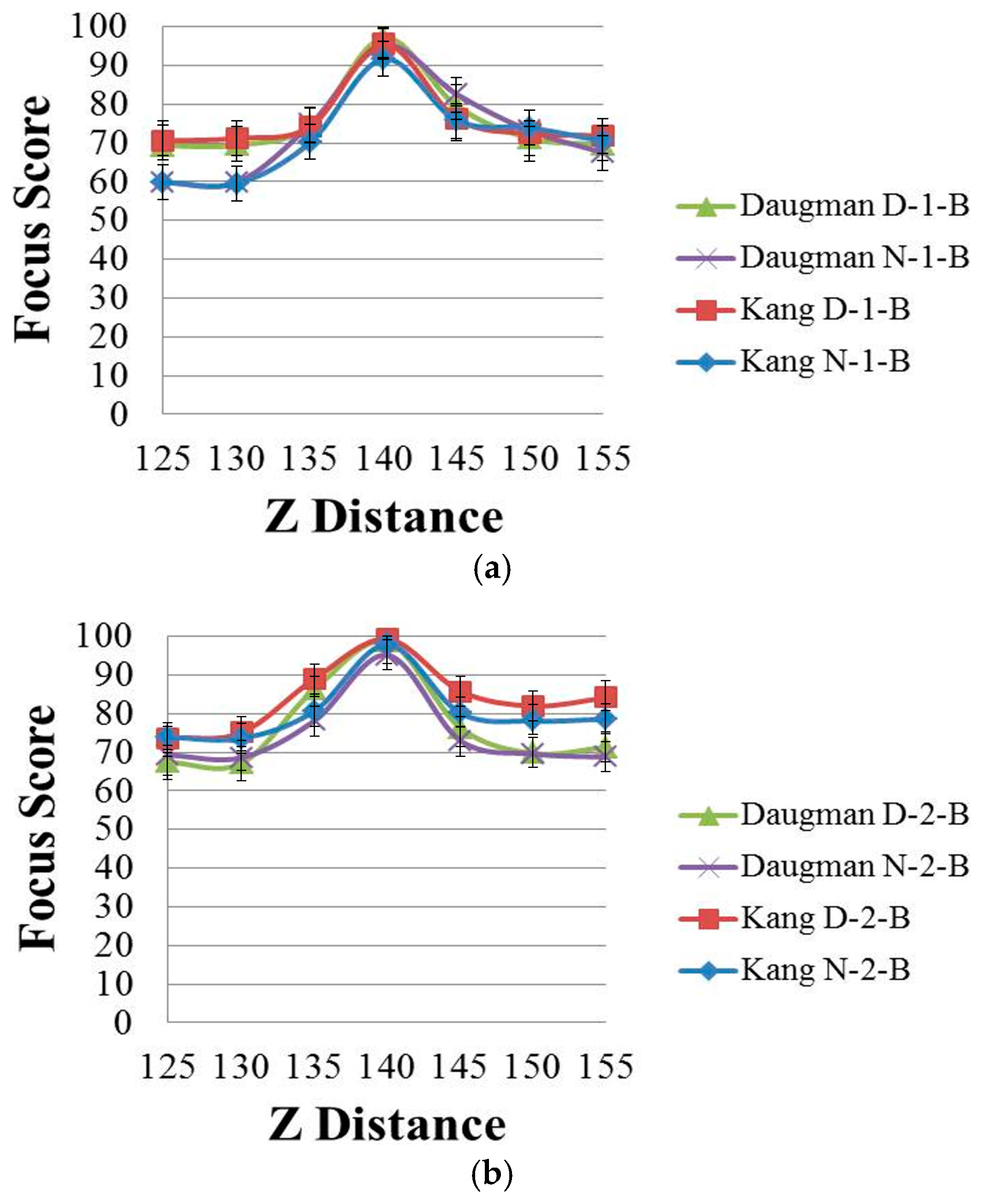
Figure 3 shows the focus score graphs of the same object of the eye region according to the Z distance, and it represents the performances of spatial domain methods before using linear normalization. In Figure 3 the most focused image can be obtained at a position of 140. The “Daugman D-1-B” graph is the result achieved by Daugman’s mask [9] using the daytime images in Database 1, whereas the “Daugman N-1-B” graph is the result achieved by Daugman’s mask using the nighttime images in Database 1. The “Kang D-1-B” graph is the result achieved by Kang’s mask [10] using the daytime images in Database 1, whereas the “Kang N-1-B” graph is the result achieved by Kang’s mask using the nighttime images in Database 1. Following the same notation, “Daugman D-2-B”, “Daugman N-2-B”, “Kang D-2-B” and “Kang N-2-B” represent the results obtained using Database 2. “D” denotes a daytime image and “N” denotes a nighttime image. “B” indicates that the results are obtained before using linear normalization. The numbers “1” or “2” represent the results obtained using Database 1 and Database 2, respectively.
Databases 1 and 2 were captured using the gaze-tracking system shown in Figure 1. All of the images were captured in both daytime and nighttime, and our databases involve a variety in brightness. Database 1 contains 84 gray images from 12 people, which were captured by the gaze-tracking camera with the f-number of 4. In addition, Database 2 contains 140 images from 20 people captured using a camera with the f-number of 10 in order to increase the DOF. However, when we captured Database 2, we increased the power of the NIR illuminators twice by increasing the number of NIR LEDs, which causes the images in Database 2 to be brighter than those in Database 1, although the f-number in Database 2 is larger. The captured image is 1600 × 1200 pixels with a gray image of 8 bits. Detailed explanations of Databases 1 and 2 are included in Section 3.1.
By comparing the four graphs of Figure 3a, even in the case of the same Z distance, the focus score with the daytime image is different from that with the nighttime image even by the same focus assessment method. For example, in Figure 3a, considering the Z-distance range of 125–140 cm, the focus score by Kang’s method with the daytime image (Kang D-1-B) is about 71 at the Z distance of 130 cm, whereas that with the nighttime image (Kang N-1-B) is about 60 at the Z distance of 130 cm. This means that the focus score has a standard deviation at each Z distance according to daytime and nighttime images, although all of the other conditions, such as the object (to be captured), camera, Z distance, focus measurement method, etc., are the same.
As shown in Figure 3a, with the nighttime image (Kang N-1-B), the Z distance becomes 135 cm (instead of 130 cm) in the case of the focus score of 71. This means that even with the same focus score (by the same focus measurement method), the calculated Z distance can be different, from 130 cm with the daytime image to 135 cm with the nighttime image, which make it difficult to estimate the accurate Z distance for auto-focusing based on the focus score. The same cases occur in the methods of Figure 3b and Figure 4a,b. Therefore, we propose a new focus measure (by combining four focus measurement methods based on ε-SVR, as shown in Figure 2), which is less affected by the variations of image brightness.
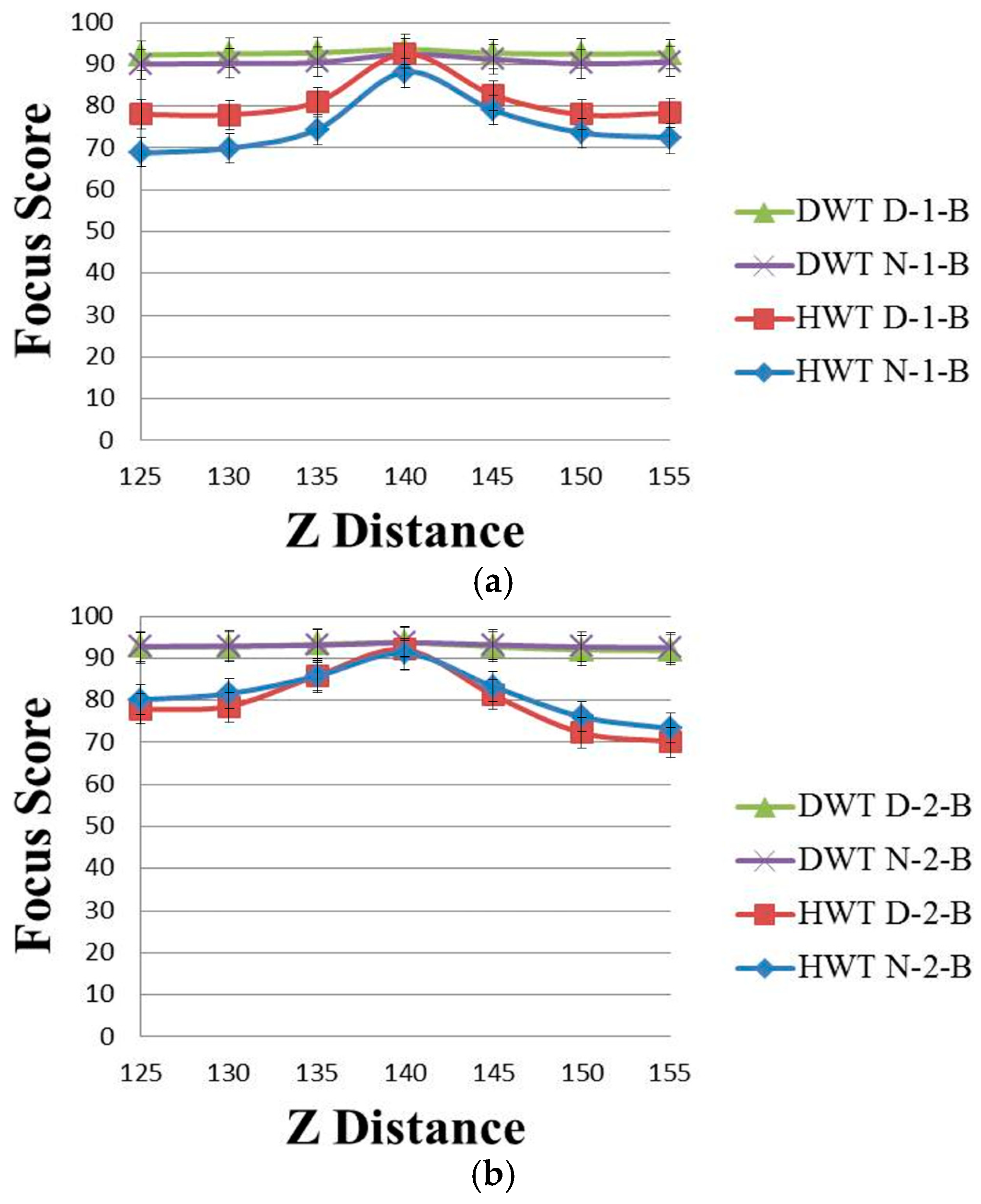
Figure 4 shows the focus score graphs of the same object of the eye region according to the Z distance of the wavelet domain methods before using linear normalization. Furthermore, in Figure 4a,b, the most focused image can be obtained at a position of 140. “DWT” and “HWT” indicate Daubechies wavelet transform and Haar wavelet transform, respectively. “D” denotes a daytime image, and “N” denotes a nighttime image. “B” indicates that the results are obtained before using linear normalization. The numbers “1” or “2” represent the results obtained using Database 1 and Database 2, respectively. In Figure 3 and Figure 4, we presented standard deviation values, as well. In all of the cases of Figure 3 and Figure 4, the standard deviation values are similar, 2.74 (minimum value)–2.92 (maximum value).
Due to the characteristics of Daubechies wavelet transform of using the longer supports of wavelets and scaling signals than Haar wavelet transform [19,21], the focus score by Daubechies wavelet transform is less affected by the illumination change in the daytime and nighttime images than that by the Haar wavelet transform. Therefore, the difference in “DWT D-2-B” and “DWT N-2-B” in Figure 4 is much smaller than that in “HWT D-2-B” and “HWT N-2-B”, and even the value of “DWT D-2-B” is the same as that of “DWT N-2-B”.
Nevertheless, in Figure 3 and Figure 4, the two main differences still observed in the focus score are the difference between daytime images and nighttime images, as well as the difference between the two databases. The difference between daytime and nighttime images is shown in Table 2, which indicates that linear normalization can reduce the difference between daytime and nighttime images. Therefore, linear normalization can decrease the effect of brightness variation on focus measurements. These differences are explained by the camera optics theory in the following discussions.
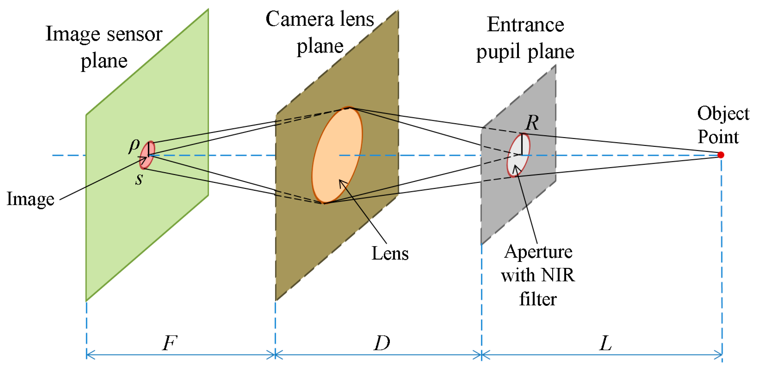
The first explanation for the difference between daytime and nighttime images is provided by the solar spectrum theory. The Sun emits electromagnetic radiation across most of the electromagnetic spectrum [22,23,24]. In our experiment, the NIR illuminators emit light of a wavelength of 850 nm, and a filter is used in the camera to prevent environmental light of other wavelengths from being incident on the camera sensor. Therefore, the light energy incident on the sensor consists of the NIR light of illuminators and a part of the NIR spectrum of solar radiation. Accordingly, we can analyze the energy incident on the camera sensor in the case that the image is focused, as shown in Figure 5.
In Figure 5, we describe an object point in the NIR light environment. The image is a circular shape in the image sensor plane according to the size of the aperture of the camera. Assuming that the photon density, I, is constant, s is the image sensor area that the point is projected on, given the aperture of size R, and ρ is the radius of the circle in the image, we obtain the equation E (image brightness) = s × I × h × ν = πρ2Ihν based on [25]. As evident in Figure 5, we obtain the equations, ρ/R = F/D, and ρ = R(F/D), where R is the radius of aperture, F is the focal length of the lens and D is the distance from the lens plane to the entrance pupil plane. Therefore, E = πR2(F2/D2)Ihν = R2I × (πF2hν/D2). In the case that the image is focused, D is fixed, and F is a constant. If the constant M denotes π F2hν/D2, we can obtain the following equation:
E = R2IM
Based on the principle that the focus level is the energy of the high frequency component in the image domain, we can divide the energy E into two parts, E = A + a, where A is the energy of the high frequency component, which defines the focus level, and a is the energy of the low frequency component, which is the so-called “blur amount”. In the case that the image is focused, the ideal image of the object point can be shown as a point. However, since the aperture is not a pinhole, a blurred region appears around the exact image point. Accordingly, we can consider that the blur amount (a) is the energy incident on the region of the image excluding the exact image point. Assume that the energy E spreads homogeneously on the image area; we can calculate A as shown in Equation (2):
where sp is the area of one pixel of image sensor. If the image is an ideally-focused one, s becomes the area of one pixel of the image sensor, and s is the same as sp. If the image is a blurred one, s becomes the area of multiple pixels of the image sensor, which is larger than sp and symmetrical based on s. Considering our previous discussion on the difference of daytime and nighttime images, we denote Ed and En as the energies incident on the sensor in the case of a daytime image and a nighttime image, respectively. Furthermore, we denote Ad and An as the focus levels of the daytime image and nighttime image, respectively. Using the same f-number to capture these images, we obtain the same radius of aperture, R. By referring to Equation (1), we obtain Ed = R2IdM, and En = R2InM. Therefore, by referring to Equations (1) and (2), we obtain Ad = R2IdM(sp/s), and An = R2InM(sp/s). As explained previously, since the energy originates from a part of the NIR spectrum of solar radiation and the NIR light of illuminators, we can rewrite these equations as Ad = R2(IdS + IdI)M(sp/s) and An = R2(InS + InI)M(sp/s), where IdS and InS denote the NIR light intensity of solar radiation during day and night, respectively; IdI and InI denote the NIR light intensity of illuminators during day and night, respectively. Since we have used the same NIR illuminators in the daytime and nighttime cases, IdI = InI = II, we obtain the following equation:
where ΔIS = IdS − InS is the difference between the light intensities of daytime and nighttime, and ΔIS is a large positive value. Therefore, Ad/An is larger than 1, and consequently, Ad is larger than An. Since A is defined as the energy of the high frequency component, which defines the focus level, we determine that the energy (Ad) of the daytime of the high-frequency component, which defines the focus level, is larger than (An) of the nighttime of the high-frequency component, which also defines the focus level. Therefore, the focus scores of daytime images are usually higher than those of nighttime images, as shown in Figure 3 and Figure 4.
A = E(sp/s)
Ad/An = (IdS + II)/(InS + II) = 1 + ΔIS/(InS + II)
In addition, in Equation (3), if II is much larger than InS, ΔIS/(InS + II) is almost 0, and Ad/An is close to 1, which indicates that the focus scores of the daytime images can be similar to those of nighttime images. Since we used a brighter NIR illuminator while collecting Database 2 compared to Database 1 (see Section 3.1), II of Database 2 is larger than II of Database 1, and the consequent difference between the focus scores of daytime images and nighttime images is smaller in Database 2 compared to that in Database 1, as shown in Figure 3 and Figure 4.
The second explanation is regarding the difference between the two databases. Ignoring the difference between daytime and nighttime images, we consider the focus amounts A1 and A2 of Databases 1 and 2, respectively. Based on Equations (1) and (2), we obtain A1 = R12I1M(sp/s1), and A2 = R22I2M(sp/s2). In our experiments, Database 1 is captured using a camera of f-number 4, whereas Database 2 is acquired using a camera of f-number 10. Further, the f-number is usually proportional to the ratio of the focal length of the lens to the diameter of aperture. As shown in Figure 5, R is the radius of aperture, and F is the focal length of the lens. Therefore, F/R1 = 4 in the case of Database 1, and F/R2 = 10 in the case of Database 2, which implies R1 = (10/4)R2 = 2.5R2. As shown in Figure 5, ρ is proportional to R. Therefore, ρ1 = 2.5ρ2, which results in s1 = 2.52s2 because s = πρ2, as shown in Figure 5. In our experiments, the power of illuminators in Database 2 is twice that in Database 1, which implies, II1 = 0.5II2. Assuming that the NIR energy of solar light is constant:
I1 = IS + II1 = (IS + II2) − 0.5II2 = I2 − 0.5II2
Accordingly, we obtain the following equation:
The relationship between A1 and A2 is shown as follows:
Based on Equations (5) and (6), we can conclude that the high frequency components of Database 2 (A2) are larger than those of Database 1 (A1). The difference between these two high frequency components is ΔA = 0.5II2hνsp, which depends on the power of illuminators (II2).
Based on these two explanations, the difference between daytime and nighttime images or the brightness difference of illuminators can cause a variation of the focus score. The brightness of the illuminator can be fixed and remains unchanged if the hardware of the gaze-tracking system with an NIR illuminator is determined. Therefore, we can only consider the difference between daytime and nighttime images, and the right side of Equation (3) should be equated to 1. Accordingly, we have two options: decreasing ΔIS (= IdS − InS) or increasing II. In order to decrease ΔIS, we apply linear normalization by compensating the brightness of the entire pixels of the daytime and nighttime images to adjust the average grey-level to be the same value. The result of decreasing ΔIS can be seen in Table 2 by comparing the results of “before linear normalization” and “after linear normalization”. On the other hand, in order to increase II, we increase the power of illuminators in the gaze-tracking system. The result of this work is Database 2, in which we set the power of the illuminator to be two-times larger than that of the illuminator in Database 1. Figure 3 and Figure 4 show that the difference between daytime and nighttime images in Database 2 is smaller than that in Database 1. This result can be also observed in Table 2. The last right column (“Database 2” and “after linear normalization”) of Table 2 describes the result of decreasing ΔIS and increasing II, simultaneously.
In these derivations, we attempt to confirm that the high frequency components (A2) of daytime images are theoretically larger than those (A1) of nighttime images if not considering other factors. To prove this, all of the mentioned factors of object distance, image distance, point spread function, etc., are actually set to be the same in both daytime and nighttime images of our experiments. Through this simplified derivation, in the case that all of the mentioned factors are the same, we found that the variation of high frequency components in the captured images even at the same position of Z distance can be reduced by decreasing the brightness change of captured images (ΔIS of Equation (3)), and it can be done by our linear normalization method. Considering that all of these factors for this theoretical derivation are so complicated, and we would do this derivation considering all of these factors in future work.
2.3. Four Focus Measurements
As explained in Section 2.1 with Figure 2, four separate focus scores are used as the inputs to ε-SVR in our method. In order to calculate the focus scores, we use two spatial domain-based methods: Daugman’s symmetrical convolution kernel [9] and Kang’s symmetrical convolution kernel [10]. In addition, two wavelet domain-based methods are used: the ratio of high-pass and low-pass bands of DWT [11] and that of HWT.
A defocused image can be usually described as a convolution of a focused image by a 2D point-spread function (PSF) defined by a Gaussian function, whose sigma value is proportional to the defocus level. Daugman considered the PSF as an isotropic (symmetrical) Gaussian function, and in the 2D Fourier domain, a defocused image is the product of a focused image and the Gaussian function of defocusing. Daugman’s convolution kernel is an 8 × 8 pixel mask, shown in Figure 6a, and it is a band-pass filter that accumulates the high frequency components of the image. The summated 2D spectral power measured by the convolution kernel was passed through a compressive nonlinearity equation in order to generate a normalized focus score in the range of 0–100 [9]. In our method, the focus score is scaled into the range of 0–1 for the input of ε-SVR.
Kang’s convolution kernel improves the performance of Daugman’s method [10]. The size of Kang’s mask is 5 × 5 pixels, as shown in Figure 6b, which achieves a smaller processing time than Daugman’s mask. Similar to Daugman’s mask, Kang’s mask has the symmetrical shape. It collects the total high frequency energy of the input image, which is passed through a nonlinear normalization. Thus, the focus score is represented in the range of 0–100, and we re-scale the score into the range of 0–1 for the input of ε-SVR.
In the wavelet domain-based method, the more focused the image, the larger the focus score [16]. Since the wavelet transform requires a square-sized image, a change of image width or height is needed. In our work, the size of the captured images is 1600 × 1200 pixels, and their size is changed into 1024 × 1024 pixels for DWT and HWT by bi-linear interpolation, whereas the original image can be used for the spatial domain-based method of focus measurement. Consequently, the focus measure in DWT and HWT can be more erroneous owing to the change in size compared to that of the spatial domain-based method.
The procedures used for DWT and HWT in our method are the same. When an input image with the dimensions of is decomposed by the wavelet transforms with a level of n and a multiplicity of m, we can obtain high-pass sub-bands and low-pass sub-bands with the dimensions of . In the proposed method, we collect the ratios of the average values per pixel in the high-pass () and low-pass sub-bands () of the four levels of the transformed image, as shown in Equation (7).
where F denotes the focus score of the image and wi represents the weight at the i-th level index. HHi and LLi are the high frequency (in both horizontal and vertical directions) sub-band and low frequency (in both horizontal and vertical directions) sub-band, respectively, at the i-th level index. The weight is required because the values of high-high (HH) components are very small and decrease according to the level of transformation. The focus score is passed through nonlinear normalization to obtain a focus score in the range of 0–1.
2.4. ε-Support Vector Regression with a Symmetrical Gaussian Radial Basis Function Kernel for Combining Four Focus Scores
Using four individual methods of focus measurement, we propose a method to use ε-SVR with a symmetrical Gaussian RBF kernel to combine the information from both spatial and wavelet domain-based methods, as shown in Figure 2. The output of our architecture is the combination of the four input focus scores obtained from the four individual methods. Consequently, the accuracy of the focus assessment can be increased. In the four individual focus measurements, the focus score graphs vary according to the users. The variation of the focus score graph leads to an error in auto-focusing. However, the reasons for an error in one method may be different from those of other methods, and they do not affect each other. Therefore, we utilize the advantages of one of these four methods to overcome the errors in the other methods by using a suitable combiner.
Various methods can be considered as the combiner, including SVR [26,27,28,29], linear regression (LR) [30] and multi-layered perception (MLP) [31,32,33,34,35,36]. SVR represents the decision boundary in terms of a typically small subset of all training examples [28]. This algorithm seeks estimation functions based on independent and identically distributed data. This type of SVR is called ε-SVR because it uses an ε-insensitive loss function proposed by Vapnik [26]. The parameter ε is related to a specific level of accuracy. This detail makes ε-SVR different from the subsequent proposed method of ν-SVR in [28]. In the proposed method, we use focus values of four individual measurements as the input for ε-SVR to obtain the final focus score. The experimental result using our two experimental databases shows that ε-SVR performs better than ν-SVR, LR, and MLP (see Section 3).
Contrary to SVM, which deals with the output of {±1}, SVR is a regression estimate concerned with real-valued estimating functions [27]. Vapnik proposed ε-SVR, including ε-insensitive loss functions; L(y, f(xi, α)) = L(|y − f(xi, α)|ε), where y is the output, xi is the input pattern, α is a dual variable and f(xi, α) is the estimation function. |y − f(xi, α)|ε is zero if |y − f(xi, α)| ≤ ε, and the value of (|y − f(xi, α)| − ε) is obtained otherwise [26]. In order to estimate the regression function using SVR, we adjust two parameters: the value of ε-insensitivity and the regularization parameter C with the kernel type [27]. There are many types of kernel functions used in ε-SVR, such as linear, polynomial, sigmoid, RBF kernels, etc. In our research, we compared the accuracies of various kernels (see Section 3), and we used the RBF kernel in ε-SVR. The RBF kernel is described as a symmetrical Gaussian function, . With training data, the parameter γ is optimized to the value of 0.025. By changing the value of ε, we can control the sparseness of the SVR solution [27]. In our research, we set ε to be the optimal value of 0.001 with training data, and the regularization parameter C is set to 10,000.
Figure 7 shows the proposed architecture of ε-SVR with RBF. The input vectors, xt, consist of four elements, which are the focus scores obtained by four individual methods: Daugman’s kernel, Kang’s kernel, DWT and HWT. The input vectors (xi) are mapped through mapping function Φ(xi) onto the feature space, where the kernel function RBF can be computed. Φ(xi) is used for mapping the input vector (xt) in low dimension into the vector in high dimension. For example, the input vector in 2 dimensions is transformed into that in 3 dimensions by Φ(xi). That is because the possibility of separating the vectors in higher dimensions is greater than those in lower dimensions [26,27,28,29]. The function of Φ(xi) is not determined as one type, such as the sigmoid function, and any kinds of non-linear function can be used. The mapped vectors are sent to the symmetrical Gaussian RBF kernel: k(xi, x) = RBF(Φ(xi), Φ(x)). Subsequently, the kernel function values are weighted with wi to calculate the output focus score (fsout). In the last step, the weighted kernel function values are summed into the value P (=Σi(wi k(xi, x))), and subsequently, P is passed to the linear combination for the regression estimation fsout = σ(P) = P + b, where b is a scalar real value.
The ideal graph of the focus score according to the Z distance should be a linearly-increased one from 125 cm to 140 cm, whereas it should be a linearly-decreased one from 140 cm to 155 cm of Figure 3 and Figure 4. Based on this, we determine the desired output for the training of ε-SVR. For example, with the image captured at the position of the Z distance of 125 cm, the desired output is determined as 10, whereas with that of 140 cm, the desired output is determined as 100. In addition, with the image at the position of the Z distance of 155 cm, the desired output is determined as 10. In the ranges from 125 cm to 140 cm and from 140 cm to 155 cm, the desired output is determined based on two linear equations, respectively.
2.5. Criterion for Comparing Performances of Different Focus Measurement Methods
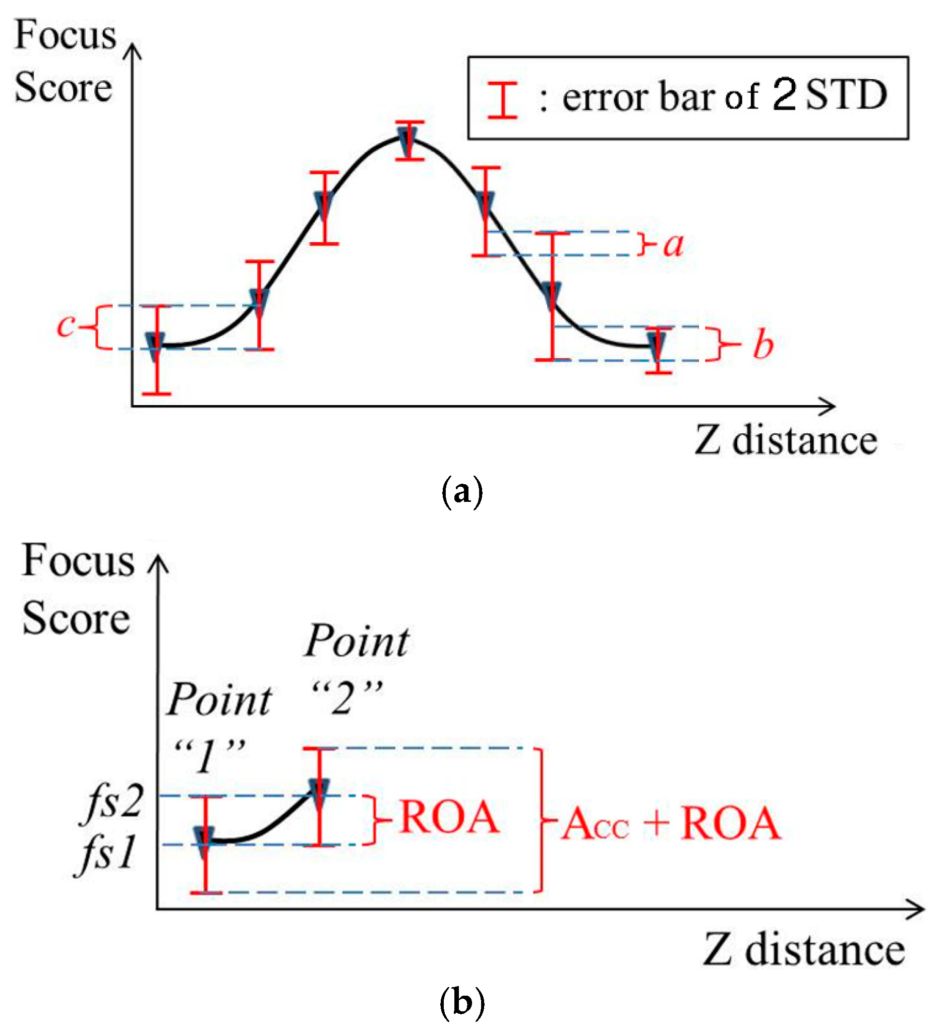
The focus score is illustrated as a graph according to the Z distance, as shown in Figure 8. At each point of image capturing, the focus score varies in the range of the error bar of 2 standard deviations (2STD). In order to adjust the focus lens, we expect the range of the error bar of each point not to overlap with that of the adjacent point. Therefore, we discovered a method that minimizes the overlapping amount. Based on the overlapping amount, we can evaluate and compare the performances of different focus assessment methods. First, we consider the relation between the focus score graph and focus lens adjustment. As shown in Figure 8a, the amounts a, b and c are the relative overlapping amount of three pairs of adjacent capturing points. When the focus score falls in these overlapping ranges, the focus assessment is inaccurate because it is impossible to decide to which capturing point the focus score belongs. The ideal graph is the one that does not include any relative overlapping amount. Unfortunately, we usually obtain high or low relative overlapping amount (ROA). We can use the ROA to evaluate the performances of the focus score graphs. Figure 8b illustrates the method to calculate ROA as follows:
where gradient1,2 = fs2 − fs1. The accurate amount (ACC) is the range from the lower terminal of Point 1 to the upper terminal of Point 2 restricting the ROA as follows, shown in Figure 8b.
The proposed criterion, which is the so-called “performance evaluation ratio” (PER), can be defined as follows, shown in Figure 8b.
PER = ROA/(ACC + ROA)
Generally, we calculate the PER between two adjacent points of image capturing based on Equations (8)–(10) as shown in Equation (11):
As shown in Figure 8b, negative or zero ROA indicates that there is no error in controlling the focus lens from the i-th point to the (i + 1)-th point. As shown in Equation (11), if ROA is negative or zero, PER is negative or zero, respectively. Therefore, we can also expect that negative or zero PER indicates that there is no error in controlling the focus lens from the i-th point to the (i + 1)-th point. If ROA is positive, PER is also positive. Therefore, we can also expect that positive PER indicates that there is an error in controlling the focus lens from the i-th point to the (i + 1)-th point.
Equation (11) shows only the PER value between two adjacent points (the i-th point and the (i + 1)-th point), and the average PER in all of the points is used as the criterion for comparing the performance of various focus measurement methods as shown in Equation (12):
where N + 1 is the number of all of the points of image capturing in the graph of the average focus score to the Z distance of Figure 8.
Because it is difficult to quantitatively compare the performances of various focus measurement methods just with the graphs of the average focus score to the Z distance, we propose the average PER value as a new criterion for performance the comparison. In conclusion, PER is a just criterion for comparing the performances of various focus measurement methods, as shown in Table 3, Table 4 and Table 5, and it is not used for the actual auto-focusing operation.
3. Experimental Results
3.1. Two Experimental Databases
In our experiment, two databases were gathered by our lab. These databases were captured using the gaze-tracking system shown in Figure 1. All of the images were captured in both daytime and nighttime, and our databases involve variety in brightness. The brightness of an image can be changed by various factors, such as time, location, illuminations and the characteristics of the camera. Further, an important characteristic of a camera is the f-number, which shows the characteristics of the trade-off between the image intensity and DOF [8]. When the f-number is larger, we obtain a darker image and a longer DOF, which results in the difference between the two databases. Database 1 contains 84 gray images from 12 people, which were captured by the gaze-tracking camera with the f-number of four. In addition, Database 2 contains 140 images from 20 people captured using a camera with the f-number of 10 in order to increase the DOF. However, when we captured Database 2, we increased the power of the NIR illuminators twice by increasing the number of NIR LEDs, which causes the images in Database 2 to be brighter than those in Database 1, although the f-number in Database 2 is larger. The difference in f-number leads to Database 1 being more sensitive to user movement than Database 2 because the DOF in Database 1 is smaller than that in Database 2. Regarding the user movement, seven images were captured for each person with one focused image at the focus point (the Z distance of 140 cm), three blurred images behind the focus point (farther from camera) and three blurred images ahead of the focus point (closer to camera). In detail, seven images were captured at the Z distances of 125, 130, 135, 140, 145, 150 and 155 cm from the camera to the human eye. Further, the ground-truth Z distance was measured using a laser distance measurement device [37]. This scheme of user movement is used in both Databases 1 and 2. The captured image has a size resolution of 1600 × 1200 pixels with a gray image of eight bits. The examples of Databases 1 and 2 are shown in Figure 9.
Based on the two-fold cross-validation scheme, which has been widely used, half of Database 1 was used for training and the other half for testing as the first trial. Then, as the second trial, the training and testing data were exchanged with each other, and training/testing are performed again. From these two trials, we obtained two experimental values and used the average one in our experiment. The same procedure was repeated with Database 2, also. Therefore, each method was trained and tested for each dataset separately because the camera and illuminator specification (f-number of 10 and twice the number of illuminators) of Database 2 are different from those of Database 1.
3.2. Performance Comparison of Various Focus Measurement Methods
Table 2 shows the performance of the linear normalization to reduce the effect of brightness variation. The values in Table 2 represent the average difference between the focus score of daytime and nighttime images in the two experimental databases. After applying linear normalization, the difference between the focus scores of daytime and nighttime images is decreased. In Table 2, we can observe that the difference between the focus scores of daytime and nighttime images in Database 2 is smaller than that in Database 1. The reason for this result is discussed in the aforementioned Section 2.2 about linear normalization.
Subsequently, we compared the performances of the four spatial domain methods in order to choose two methods as the inputs to ε-SVR. Figure 10 shows the graphs of the focus score according to the Z distance of four spatial methods—Daugman [9], Kang [10], LoG [12] and entropy [13]—and two wavelet domain methods: DWT [11] and HWT [18].
As shown in Figure 10, the performances of LoG and entropy are lower than those of other methods (the graphs obtained using LoG and entropy are less affected by the change of the Z distance compared to the other methods). In order to quantitatively measure the performances of these methods, we measured the average PERs described in Equation (12) for all of the methods, as shown in Table 3. As explained in Section 2.5, the smaller the PER, the better the method. We can easily determine that Daugman and Kang methods, DWT and HWT are better than the LoG and entropy methods. Therefore, we choose the four methods—Daugman and Kang methods with DWT and HWT—as the four inputs to ε-SVR.
3.3. Performance Comparison of Various Regressions with Four Focus Measurements
Subsequently, we performed comparative experiments with MLP, ν-SVR, LR and ε-SVR with different kernels using the same inputs of four focus measurements: Daugman [9], Kang [10], DWT [11] and HWT [18]. In our experiment, we implemented ε-SVR and ν-SVR using four kernels: RBF, polynomial, linear and sigmoid. In addition, MLP is implemented using three kernels: linear, hyperbolic tangent and general sigmoid. As explained in Section 2.4, the ideal graph of the focus score according to the Z distance should be a linearly-increased one from 125 cm to 140 cm, whereas it should be a linearly-decreased one from 140 cm to 155 cm in Figure 11. Based on this, we determine the desired output for the training of SVR and MLP. For example, with Figure 11b, with the image captured at the position of the Z distance of 125 cm, the desired output is determined as 10, whereas with that of 140 cm, the desired output is determined as 100. In addition, with the image at the Z distance of 155 cm, the desired output is determined as 10. In the ranges from 125 cm to 140 cm and from 140 cm to 155 cm, the desired outputs are determined based on two linear equations, respectively. The focus score graphs of these regressions and neural networks are shown in Figure 11.
The graphs in Figure 11 are very similar, and it is difficult to determine the best method among them. Therefore, we use the average PER of Equation (12) to evaluate these graphs. As explained in Section 2.5, the smaller the PER, the better the method. Table 4 shows the PER values of ε-SVR, ν-SVR, LR and MLP using different kernels with the two databases.
In Table 4, ε-SVR with RBF shows the smallest PER in both databases. Therefore, we can confirm that the focus assessment performance of our proposed method using ε-SVR with the RBF kernel is higher than that of other regression methods with various kernels.
3.4. Performance Comparison of Proposed Method and Four Individual Methods of Focus Measurement.
Figure 12 shows the focus score graphs of the proposed method using ε-SVR with the RBF kernel and the four individual methods of focus measurement: Daugman [9], Kang [10], DWT [11] and HWT [18]. In addition, Table 5 shows the average PER values of Equation (12) of these methods. Because the four focus scores (input vectors, xt of Section 2.4) by Daugman’s mask, Kang’s mask, Daubechies and Haar wavelet transform are not linearly changed according to the change of the Z distance, as shown in Figure 12, and these vectors are passing through nonlinear mapping function (Φ(xi) of Section 2.4) and nonlinear target function of RBF (k(xi, x) of Section 2.4), the graphs of Figure 12 can be linear or nonlinear.
As shown in Figure 12, the graph of the proposed method is affected more by the Z distance compared to the other methods. As explained in Section 2.5, the smaller the PER, the better the method. In Table 5, the proposed method exhibits the smallest PER values in both databases and in the average of the two databases. Based on Figure 12 and Table 5, we can confirm that the proposed method can enhance the focus assessment performance compared to the four individual methods: Daugman [9], Kang [10], DWT [11] and HWT [18].
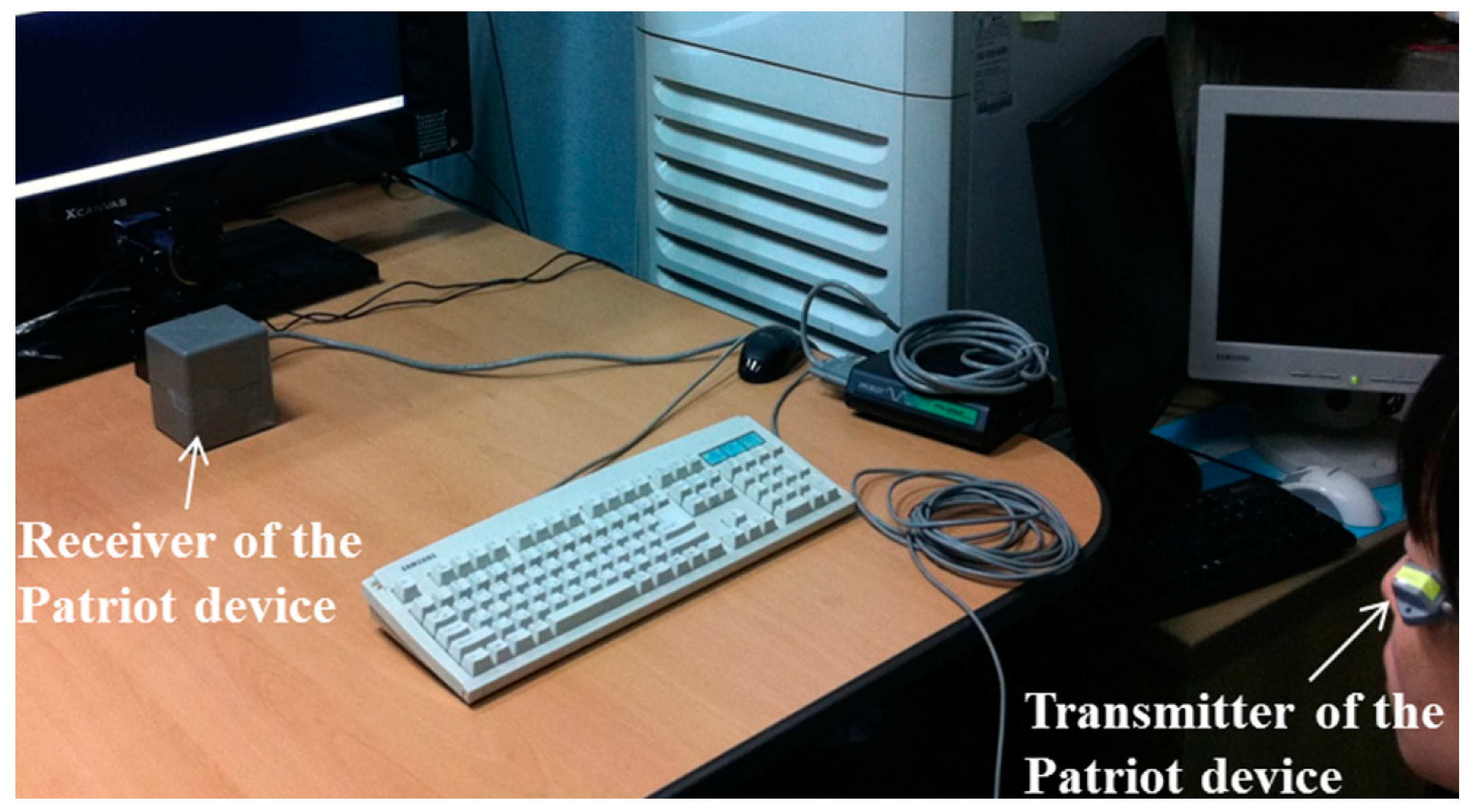
As the next experiment, we measured the accuracy of estimating the Z distance by proposed or previous focus measurement methods. For the experiment, a total of 20,000 image frames were obtained from 20 people at Z distances of 1.25–1.55 m (10,000 frames in daytime and another 10,000 frames in nighttime). Ground-truth Z distances were measured by a Polhemus Patriot 3-D motion tracking device [38]. By positioning the receiver close to the camera lens and attaching the transmitter of the Patriot device near the user’s left eye, we could obtain the ground-truth Z distance between the receiver and transmitter, as shown in Figure 13. The disparity of position between the camera lens and the receiver of the Patriot device was compensated. The accuracy of the Z distance estimation was evaluated based on the mean absolute error (MAE) of Equation (13) between the ground-truth Z distance and the Z distance obtained by proposed or previous focus measurement methods.
Z(i) and Z’(i) are respectively the ground-truth Z distance and Z distance estimated by the proposed or previous methods. M is the total number of image frames. As shown in Table 6, we can find that the accuracy of the Z distance estimation by our method is higher than those by previous methods.
3.5. Auto-Focusing Based on Our Focus Measurement Method
In our method, the initial rough position of the Z-distance of the user’s eye is estimated based on the width of the detected face in the captured image. As shown in the right bottom image of Figure 1a,b, by using a wide-view camera, the user’s face image is captured, and the face region is detected by the AdaBoost face tracker [39]. Based on the assumption that the rough (actual) widths of people’s faces are similar, the rough Z distance can be estimated based on the actual width, the width of the face detected in the image and the camera focal length. In our system, the information of the camera focal length is successively transmitted to our desktop computer via serial communication at a speed of 9600 bits per second (bps). In addition, the position of focus lens and the movement commands are transmitted to the focus motor by serial communication of same speed. Then, as shown in the right top image of Figure 1a, the focus motor rotates the ring of the focus lens (attached on the narrow-view camera), and the focus lens moves forward or backward in order to capture a focused image. Therefore, the camera focal length can be obtained based on the position of the focus lens, and consequently, the rough Z distance of the user’s eye can be obtained.
However, because there exist individual variances among the actual width of people’s face, the rough position of the Z distance calculated is not accurate. Therefore, our system performs the procedure of additional auto-focusing based on the graph of the focus score according to the Z distance, like Figure 11 and Figure 12. In detail, at the rough position of the Z distance measured by the user’s face, the focus score of the captured eye image is calculated by our focus measurement method. If the score is less than the threshold (in our research, we set the threshold as 85, which is experimentally determined based on the possibility of detecting the pupil center and corneal SR center for gaze detection), our system sends the movement command of the focus lens to the farther direction compared to the current position of the Z distance by units of 2 cm. For example, in the case of the current position of 130 cm, the lens is moved to the position that corresponds to the Z distance of 132 cm. Then, at this position, our system captures the eye image and calculates the focus score again. If the score is higher than that in the previous position (130 cm), but it is still less than the threshold (85), this procedure is repeated until the focus score of the captured eye image is higher than the threshold. If it is lower than that in the previous position, our system sends the command to move the focus lens to the closer direction (128 cm) compared to the current position, and this procedure is repeated until the focus score of the captured eye image is higher than the threshold.
Experiments for measuring the time of auto-focusing were performed with 20 people having 10 trials. During the experiments, the participating subjects were not asked to hold their head still, but gazed at nine reference positions (on the TV display of Figure 1a) by natural movement of the head and eye. Experimental results showed that the average focusing time (obtaining the focused image whose focus score is higher than 85) by our method is about 81.9 ms (81.5 ms in daytime and 82.3 ms in nighttime), as shown in Table 7. Based on these results, we can find that the difference of auto-focusing time by our method is small between daytime and nighttime images. In addition, we can confirm that the speed of auto-focusing by our method is faster than those by previous methods. In previous methods [9,10,11,18], we used the same auto-focusing mechanism (explained above), except for the focus measurement method. The reason why the sub-methods took more time than our method is that more iterations (capturing image, calculating focus score, sending the command of lens movement to the focus motor and moving the focus lens) were taken by the sub-methods than our method.
Including auto-focusing time, our gaze-tracking system can be operated at the speed of about 12 frames/s based on multi-thread processing of the auto-focusing and gaze detection, where these two processes are performed in parallel operation.
As explained in Section 2.4 and Section 3.3, the ideal graph of focus score according to the Z distance should be a linearly increased one from 125 cm to 140 cm, whereas it should be a linearly decreased one from 140 cm to 155 cm of Figure 11. Based on this, we determine the desired output for the training of the proposed ε–SVR.
For the example with Figure 11b, with the image captured at the position of the Z distance of 125 cm, the desired output is determined as 10, whereas with that of 140 cm, the desired output is determined as 100. In addition, with the image at the Z distance of 155 cm, the desired output is determined as 10. In the ranges from 125 cm to 140 cm and from 140 cm to 155 cm, the desired output for the training of our ε–SVR is determined based on two linear equations, respectively. Through the training based on these desired outputs, the graph shape of our ε–SVR is closer to a linear shape (having the wider range of focus score) than those of other methods, as shown in Figure 10b and Figure 11b. In addition, even with Figure 11a compared to Figure 10a, the graph shape of our ε–SVR is closer to a linear shape (having a wider range of focus scores) than those of other methods.
If the relationship graph between the Z distance and desired output (focus score) is closer to a linear shape with high sharpness and a wider range of focus scores, the auto-focusing based on this graph is usually easier, which can increase the consequent accuracy and speed of auto-focusing [11].
All of the individual methods of focus measurement, such as Daugman’s convolution kernel, Kang’s convolution kernel, Daubechies wavelet transform (DWT), Haar wavelet transform (HWT), LoG and entropy, were not originally designed to produce the desired output (focus score) based on the linear equation because they did not perform the training procedure with the desired outputs. However, our ε–SVR was trained in order to produce the ideal focus value (the desired output based on the linear equation) at each Z distance. Therefore, it is possible to obtain a new focus score with less error without any new information added to the system by combining several methods with high error.
4. Conclusions
In this paper, we propose a new method of focus assessment by combining Daugman’s and Kang’s methods, DWT and HWT based on ε-SVR with the RBF kernel. In order to prevent the focus score from being affected by a change in image brightness, both linear and nonlinear normalizations are adopted in the focus score calculation. In addition, based on the camera optics, we mathematically prove the reason for the increase in the focus score in the case of daytime images or a brighter illuminator compared to the nighttime images or a darker illuminator. Moreover, we propose a new criterion to compare the accuracies of the focus measurement methods. This criterion is based on the ratio of the relative overlapping amount (standard deviation of focus score) between two adjacent positions along the Z-axis to the entire range of the focus score variety between these two points. The experimental results show that the proposed method for focus assessment of a gaze-tracking camera exhibits a higher performance compared to other regression methods. In comparison to the four individual methods of focus measurement, the proposed method also exhibits higher performance, which proves that the disadvantages of the four individual methods are overcome by using the ε-SVR combination. As future work, we will evaluate the performance of our method in various environments, such as auto-focusing of a surveillance camera in the outdoors, of a mobile phone camera, etc. In addition, we will consider other kinds of data fusion methods for enhancing the performance of focus measurements.
Acknowledgments
This research was supported by the Basic Science Research Program through the National Research Foundation of Korea (NRF) funded by the Ministry of Education (NRF-2015R1D1A1A01056761), in part by the Bio & Medical Technology Development Program of the NRF funded by the Korean government, MSIP (NRF-2016M3A9E1915855), and in part by the Basic Science Research Program through the National Research Foundation of Korea (NRF) funded by the Ministry of Education (NRF-2017R1D1A1B03028417).
Author Contributions
Duc Thien Luong and Kang Ryoung Park designed the overall system for focus measurement. In addition, they wrote and revised the paper. Jeon Seong Kang, Phong Ha Nguyen and Min Beom Lee helped with the comparative experiments and collecting databases.
Conflicts of Interest
The authors declare no conflict of interest.
References
- Hansen, D.W.; Ji, Q. In the Eye of the Beholder: A Survey of Models for Eyes and Gaze. IEEE Trans. Pattern Anal. Mach. Intell. 2010, 32, 478–500. [Google Scholar] [CrossRef] [PubMed]
- Duchowski, A.T. A Breadth-First Survey of Eye-Tracking Applications. Behav. Res. Methods Instrum. Comput. 2002, 34, 455–470. [Google Scholar] [CrossRef] [PubMed]
- Morimoto, C.H.; Mimica, M.R.M. Eye Gaze Tracking Techniques for Interactive Applications. Comput. Vis. Image Underst. 2005, 98, 4–24. [Google Scholar] [CrossRef]
- Zhu, Z.; Ji, Q. Novel Eye Gaze Tracking Techniques under Natural Head Movement. IEEE Trans. Biomed. Eng. 2007, 54, 2246–2260. [Google Scholar] [PubMed]
- Cho, D.-C.; Kim, W.-Y. Long-range Gaze Tracking System for Large Movements. IEEE Trans. Biomed. Eng. 2013, 60, 3432–3440. [Google Scholar] [CrossRef] [PubMed]
- Hennessey, C.; Noureddin, B.; Lawrence, P. A Single Camera Eye-Gaze Tracking System with Free Head Motion. In Proceedings of the Symposium on Eye Tracking Research & Applications, San Diego, CA, USA, 27–29 March 2006; pp. 87–94. [Google Scholar]
- Shih, S.-W.; Liu, J. A Novel Approach to 3-D Gaze Tracking Using Stereo Cameras. IEEE Trans. Syst. Man Cybern. Part B Cybern. 2004, 34, 234–245. [Google Scholar] [CrossRef]
- F-Number. Available online: https://en.wikipedia.org/wiki/F-number (accessed on 7 June 2016).
- Daugman, J. How Iris Recognition Works. IEEE Trans. Circuits Syst. Video Technol. 2004, 14, 21–30. [Google Scholar] [CrossRef]
- Kang, B.J.; Park, K.R. A Robust Eyelash Detection Based on Iris Focus Assessment. Pattern Recognit. Lett. 2007, 28, 1630–1639. [Google Scholar] [CrossRef]
- Jang, J.; Park, K.R.; Kim, J.; Lee, Y. New Focus Assessment Method for Iris Recognition Systems. Pattern Recognit. Lett. 2008, 29, 1759–1767. [Google Scholar] [CrossRef]
- Wan, J.; He, X.; Shi, P. An Iris Image Quality Assessment Method Based on Laplacian of Gaussian Operation. In Proceedings of the IAPR Conference on Machine Vision Applications, Tokyo, Japan, 16–18 May 2007; pp. 248–251. [Google Scholar]
- Grabowski, K.; Sankowski, W.; Zubert, M.; Napieralska, M. Focus Assessment Issues in Iris Image Acquisition System. In Proceedings of the International Conference on Mixed Design of Integrated Circuits and Systems, Ciechocinek, Poland, 21–23 June 2007; pp. 628–631. [Google Scholar]
- Zhang, J.; Feng, X.; Song, B.; Li, M.; Lu, Y. Multi-Focus Image Fusion Using Quality Assessment of Spatial Domain and Genetic Algorithm. In Proceedings of the Conference on Human System Interactions, Krakow, Poland, 25–27 May 2008; pp. 71–75. [Google Scholar]
- Wei, Z.; Tan, T.; Sun, Z.; Cui, J. Robust and Fast Assessment of Iris Image Quality. In Proceedings of the International Conference on Biometrics, Hong Kong, China, 5–7 January 2006; pp. 464–471. [Google Scholar]
- Kautsky, J.; Flusser, J.; Zitová, B.; Šimberová, S. A New Wavelet-based Measure of Image Focus. Pattern Recognit. Lett. 2002, 23, 1785–1794. [Google Scholar] [CrossRef]
- Bachoo, A. Blind Assessment of Image Blur Using the Haar Wavelet. In Proceedings of the Annual Research Conference of the South African Institute of Computer Scientists and Information Technologists, Bela, South Africa, 11–13 October 2010; pp. 341–345. [Google Scholar]
- Tong, H.; Li, M.; Zhang, H.; Zhang, C. Blur Detection for Digital Images Using Wavelet Transform. In Proceedings of the IEEE International Conference on Multimedia and Expo, Taipei, Taiwan, 27–30 June 2004; pp. 17–20. [Google Scholar]
- Daubechies Wavelet. Available online: https://en.wikipedia.org/wiki/Daubechies_wavelet (accessed on 25 May 2017).
- Daubechies, I. Ten Lectures on Wavelets, 1st ed.; SIAM: Philadelphia, PA, USA, 1992. [Google Scholar]
- Haar Wavelet. Available online: https://en.wikipedia.org/wiki/Haar_wavelet (accessed on 25 May 2017).
- Ultraviolet. Available online: https://en.wikipedia.org/wiki/Ultraviolet (accessed on 13 January 2017).
- Visible Spectrum. Available online: https://en.wikipedia.org/wiki/Visible_spectrum#cite_note-1 (accessed on 13 January 2017).
- Infrared. Available online: https://en.wikipedia.org/wiki/Infrared (accessed on 13 January 2017).
- Angus, A.A. A New Physical Constant and Its Application to Chemical Energy Production. Fuel Chem. Div. Prepr. 2003, 48, 469–473. [Google Scholar]
- Vapnik, V.N. The Nature of Statistical Learning Theory, 1st ed.; Springer: Berlin, Germany, 1995. [Google Scholar]
- Schölkopf, B.; Smola, A.J.; Williamson, R.C.; Bartlett, P.L. New Support Vector Algorithms. Neural Comput. 2000, 12, 1207–1245. [Google Scholar] [CrossRef] [PubMed]
- Schölkopf, B.; Smola, A.J. Learning with Kernels-Support Vector Machines, Regularization, Optimization, and Beyond, 1st ed.; The MIT Press: Cambridge, MA, USA, 2001. [Google Scholar]
- Support Vector Machines. Available online: http://www.stanford.edu/class/cs229/notes/cs229-notes3.pdf (accessed on 7 June 2016).
- Bishop, C. Pattern Recognition and Machine Learning; Springer: Berlin, Germany, 2006. [Google Scholar]
- Haykin, S. Neural Networks: A Comprehensive Foundation, 2nd ed.; Prentice Hall: Upper Saddle River, NJ, USA, 1998. [Google Scholar]
- Multilayer Perceptron. Available online: http://en.wikipedia.org/wiki/Multilayer_perceptron (accessed on 7 June 2016).
- Areerachakul, S.; Sanguansintukul, S. Classification and Regression Trees and MLP Neural Network to Classify Water Quality of Canals in Bangkok, Thailand. Int. J. Intell. Comput. Res. 2010, 1, 43–50. [Google Scholar] [CrossRef]
- Wefky, A.M.; Espinosa, F.; Jiménez, J.A.; Santiso, E.; Rodriguez, J.M.; Fernández, A.J. Alternative Sensor System and MLP Neural Network for Vehicle Pedal Activity Estimation. Sensors 2010, 10, 3798–3814. [Google Scholar] [CrossRef] [PubMed]
- Vehtari, A.; Lampinen, J. Bayesian MLP Neural Networks for Image Analysis. Pattern Recognit. Lett. 2000, 21, 1183–1191. [Google Scholar] [CrossRef]
- Patino-Escarcina, R.E.; Costa, J.A.F. An Evaluation of MLP Neural Network Efficiency for Image Filtering. In Proceedings of the International Conference on Intelligent Systems Design and Applications, Rio de Janeiro, Brazil, 20–24 October 2007; pp. 335–340. [Google Scholar]
- Laser Rangefinder DLE70 Professional. Available online: http://www.bosch-pt.com/productspecials/professional/dle70/uk/en/start/index.htm (accessed on 19 January 2017).
- “Patriot”, Polhemus. Available online: http://www.polhemus.com/?page=Motion_Patriot (accessed on 24 March 2017).
- Viola, P.; Jones, M.J. Robust Real-time Face Detection. Int. J. Comput. Vis. 2004, 57, 137–154. [Google Scholar] [CrossRef]
Figure 1.
Proposed gaze-tracking system for intelligent television (TV) interface. (a) Gaze-tracking system; and (b) detection results of pupil center and corneal specular reflection (SR) center in the captured image by narrow-view camera (displayed on the left monitor),and the detected area of the face in the captured image by wide-view camera (displayed on right monitor).
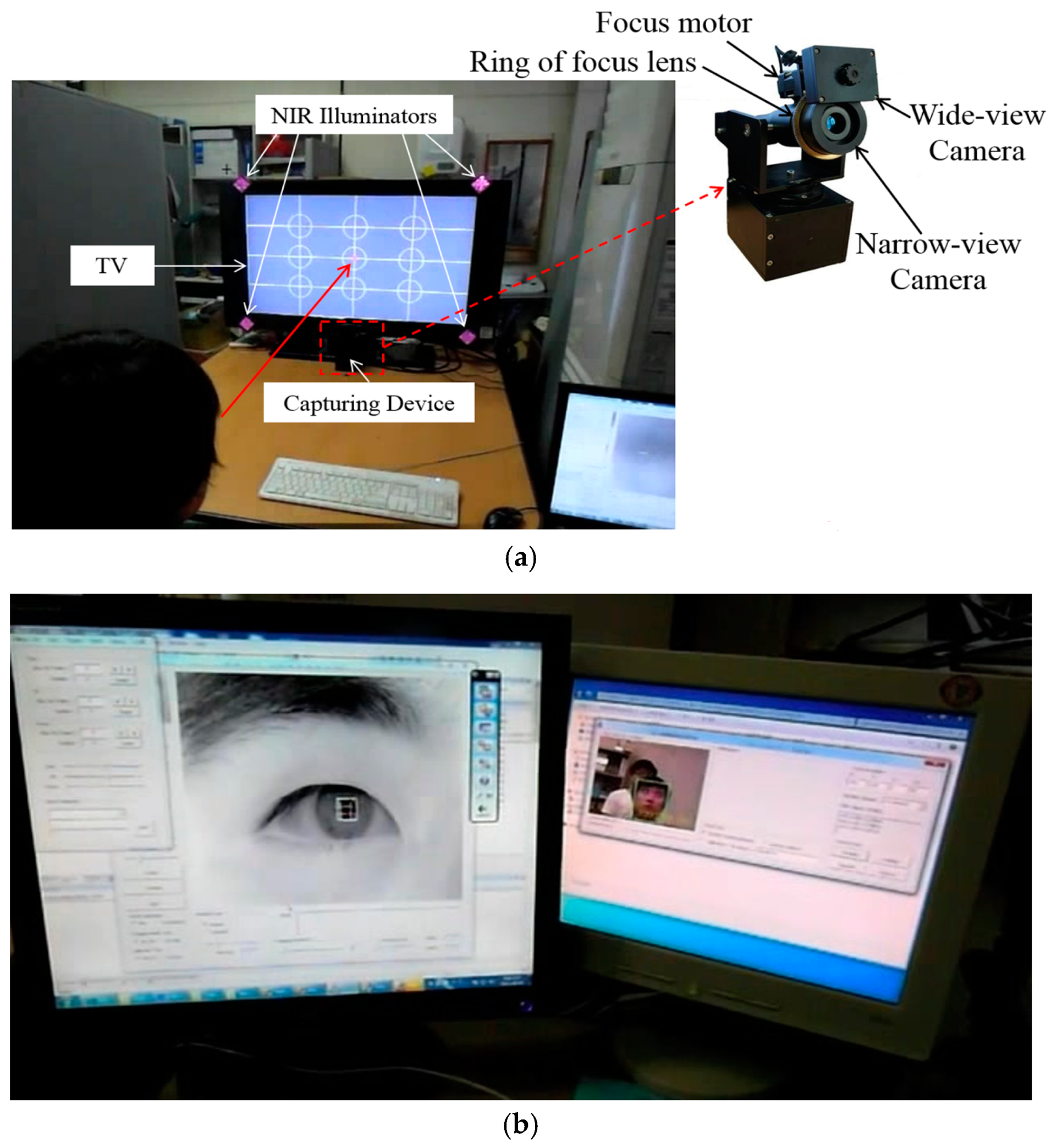
Figure 2.
Flowchart of the proposed method.
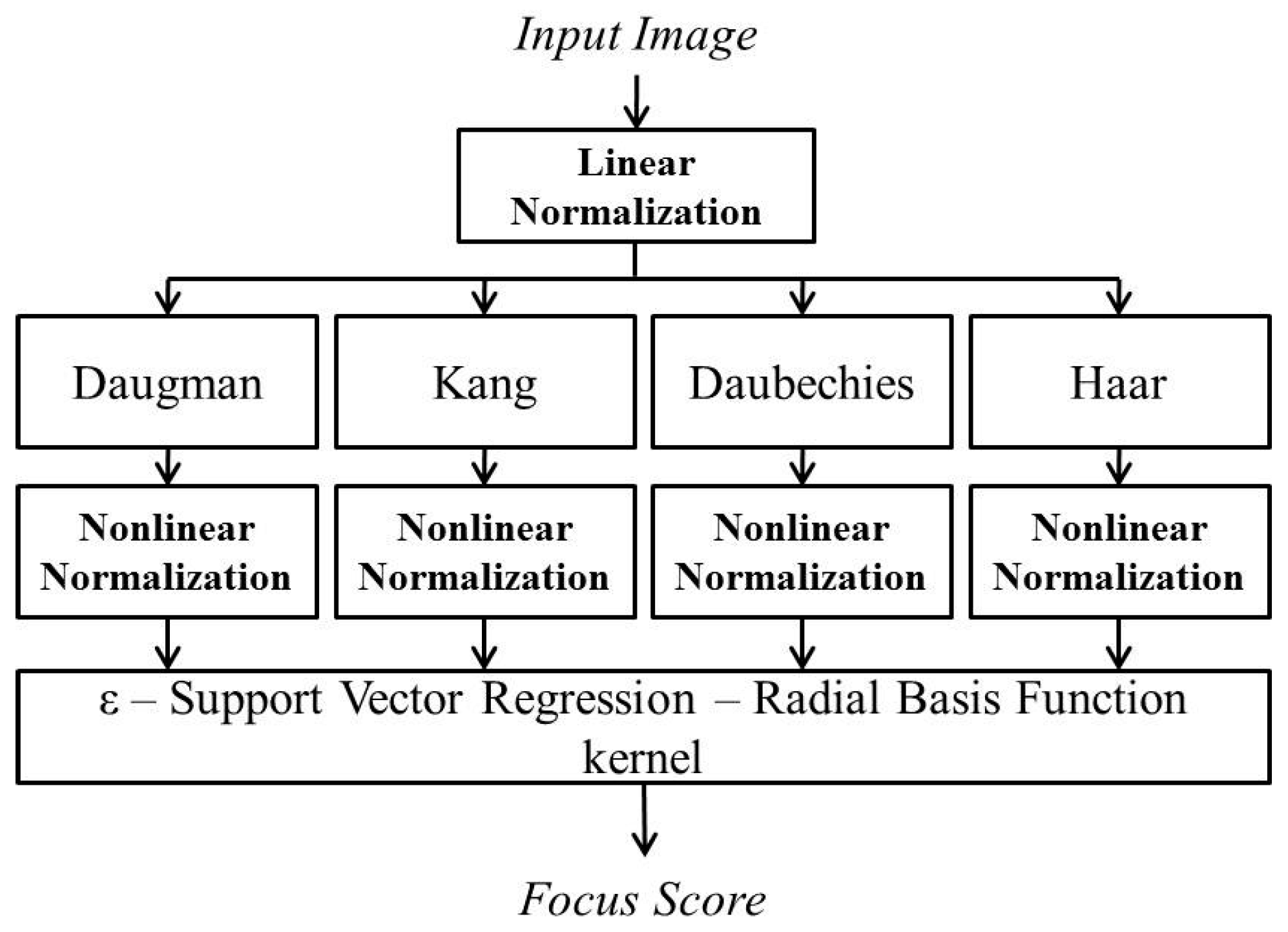
Figure 3.
The effect of brightness variation on the spatial domain methods with (a) Database 1 and (b) Database 2. “Daugman D-1-B” and “Daugman N-1-B” are the graphs by Daugman’s mask using the daytime and nighttime images in Database 1, respectively. “Kang D-1-B” and “Kang N-1-B” are the graphs by Kang’s mask using the daytime and nighttime images in Database 1, respectively. Following the same notation, “Daugman D-2-B”, “Daugman N-2-B”, “Kang D-2-B” and “Kang N-2-B” represent the results obtained using Database 2.

Figure 4.
The effect of brightness variation on the wavelet domain methods with (a) Database 1 and (b) Database 2.
Figure 4.
The effect of brightness variation on the wavelet domain methods with (a) Database 1 and (b) Database 2.

Figure 5.
Explanation of camera optics in the case that the image is focused.

Figure 6.
Symmetrical kernels for measuring the focus score in the spatial domain-based methods. (a) Daugman’s convolution kernel; and (b) Kang’s convolution kernel.
Figure 6.
Symmetrical kernels for measuring the focus score in the spatial domain-based methods. (a) Daugman’s convolution kernel; and (b) Kang’s convolution kernel.
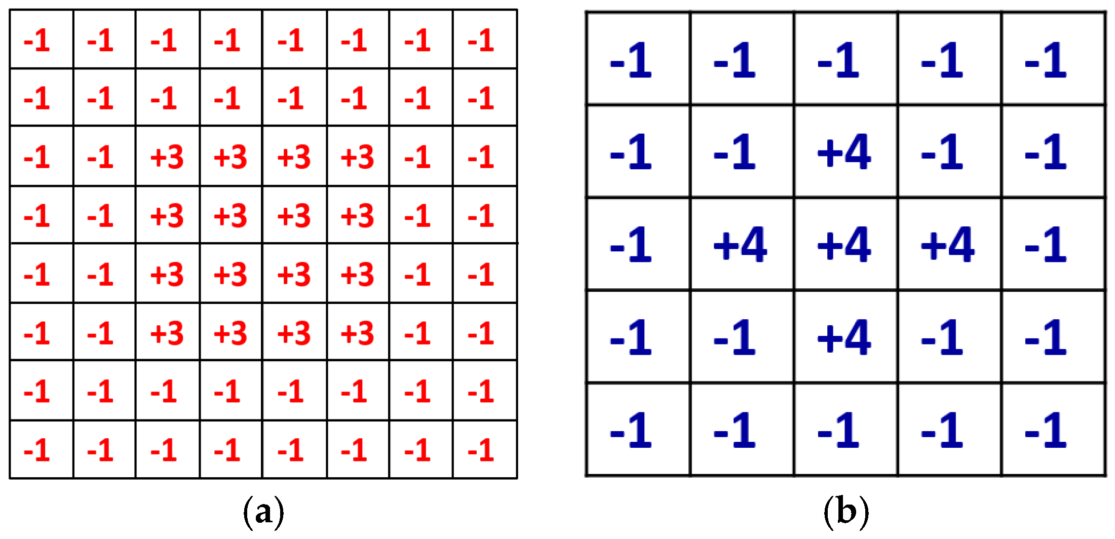
Figure 7.
ε-SVR with symmetrical Gaussian radial basis function (RBF) kernel architecture in the proposed method with four-element input vectors xt and a single output of the focus score.
Figure 7.
ε-SVR with symmetrical Gaussian radial basis function (RBF) kernel architecture in the proposed method with four-element input vectors xt and a single output of the focus score.
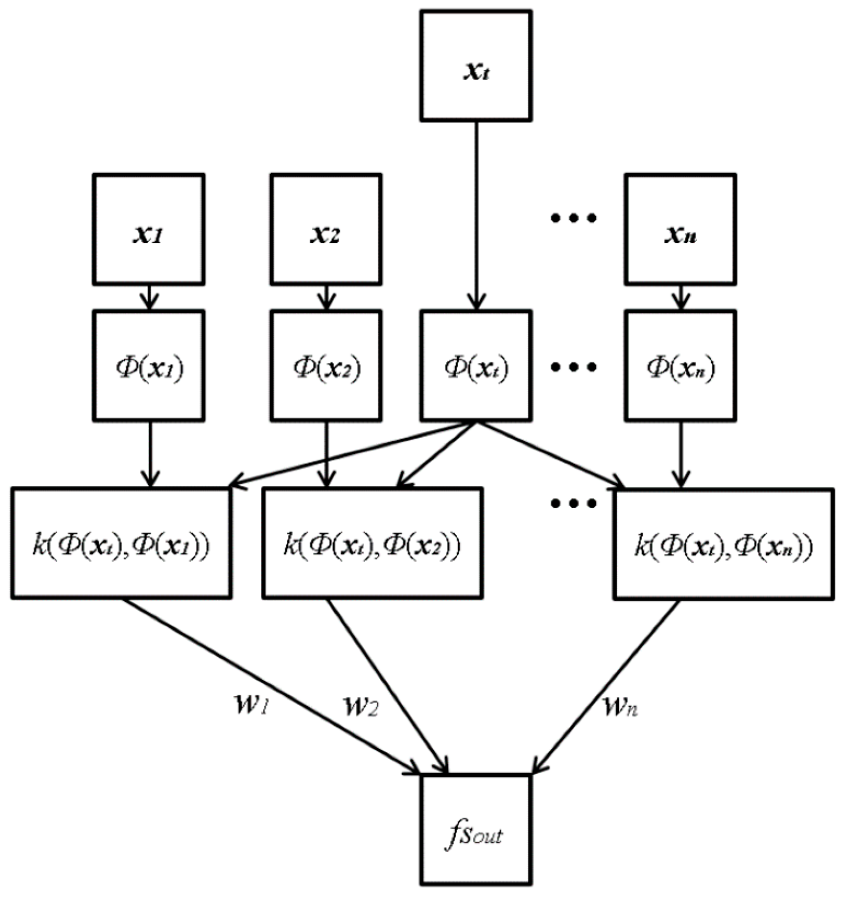
Figure 8.
An example graph of the average focus score according to the Z distance. (a) Graph with the error bar of 2 standard deviations (2STD); (b) graph with relative overlapping amount (ROA) and accurate amount (ACC) + ROA. As shown in Figure 3 and Figure 4, the capturing points are 125, 130, 135, 140, 145, 150 and 155 cm, respectively.

Figure 9.
Examples of images in Databases (a) 1 and (b) 2.
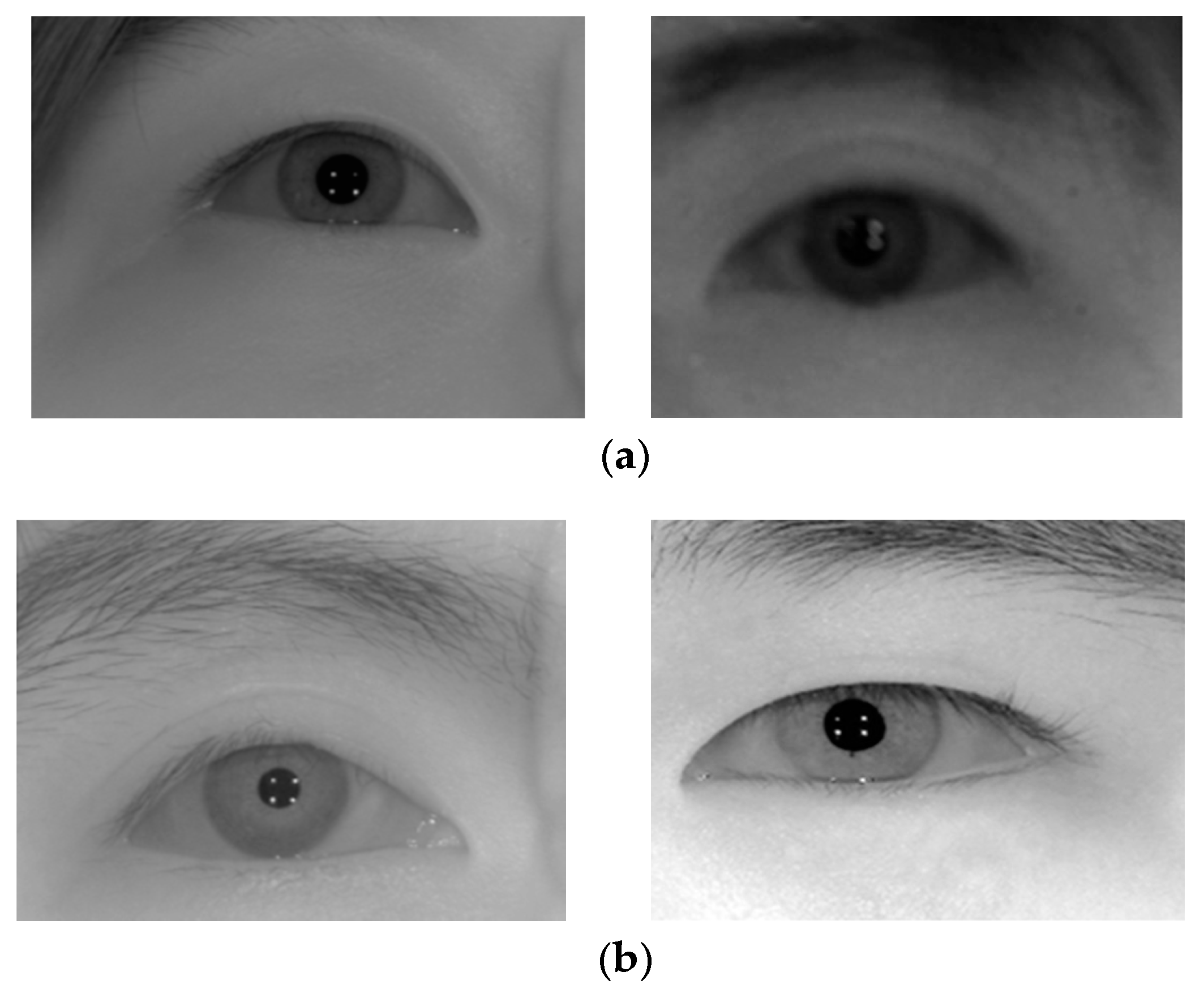
Figure 10.
Graph of the average focus score according to the Z distance of the spatial domain methods and wavelet domain methods. (a) Database 1; and (b) Database 2.
Figure 10.
Graph of the average focus score according to the Z distance of the spatial domain methods and wavelet domain methods. (a) Database 1; and (b) Database 2.
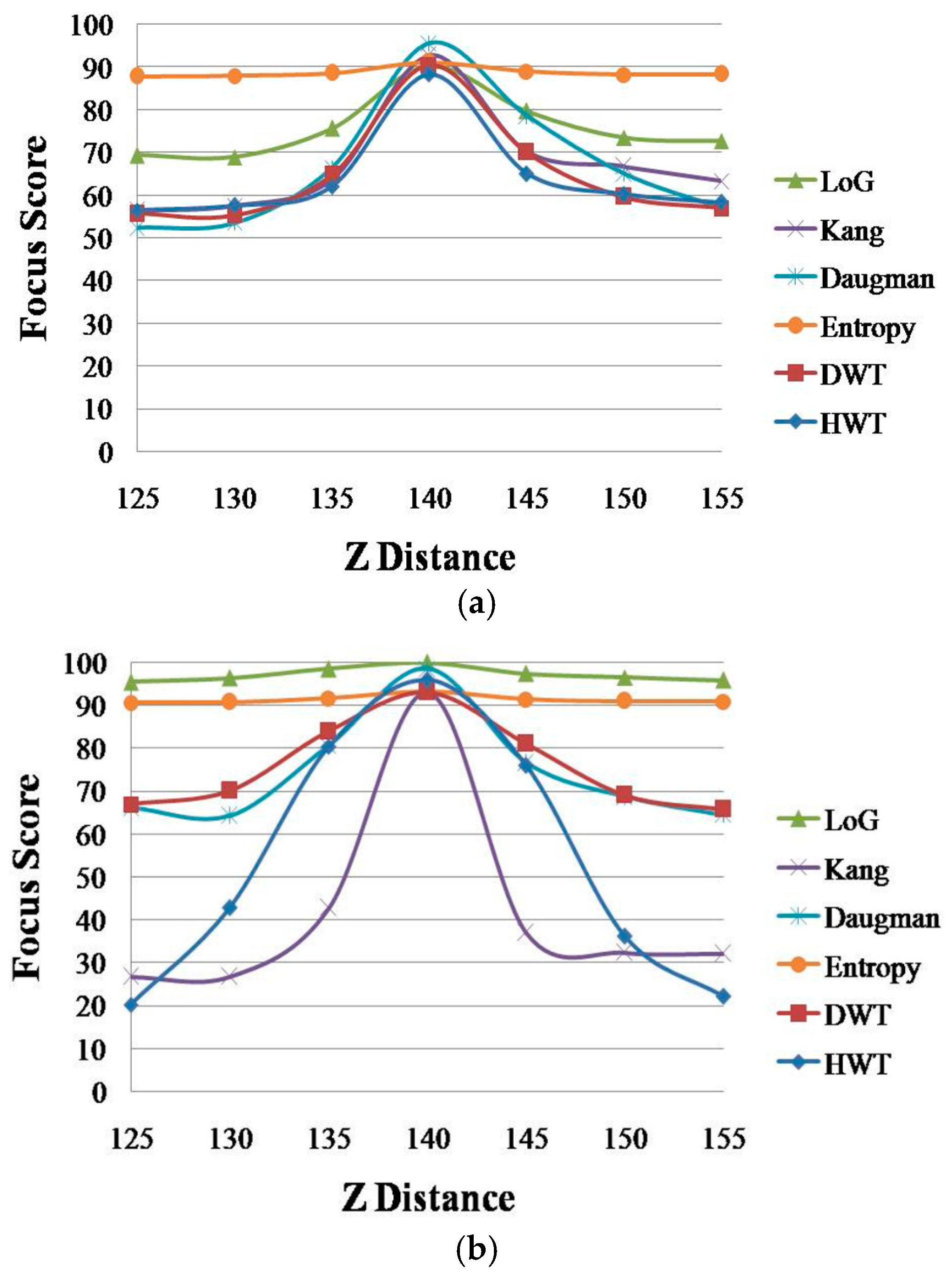
Figure 11.
The focus score graphs of ε-SVR, ν-SVR, LR and MLP using different kernels. (a) Database 1; and (b) Database 2.
Figure 11.
The focus score graphs of ε-SVR, ν-SVR, LR and MLP using different kernels. (a) Database 1; and (b) Database 2.
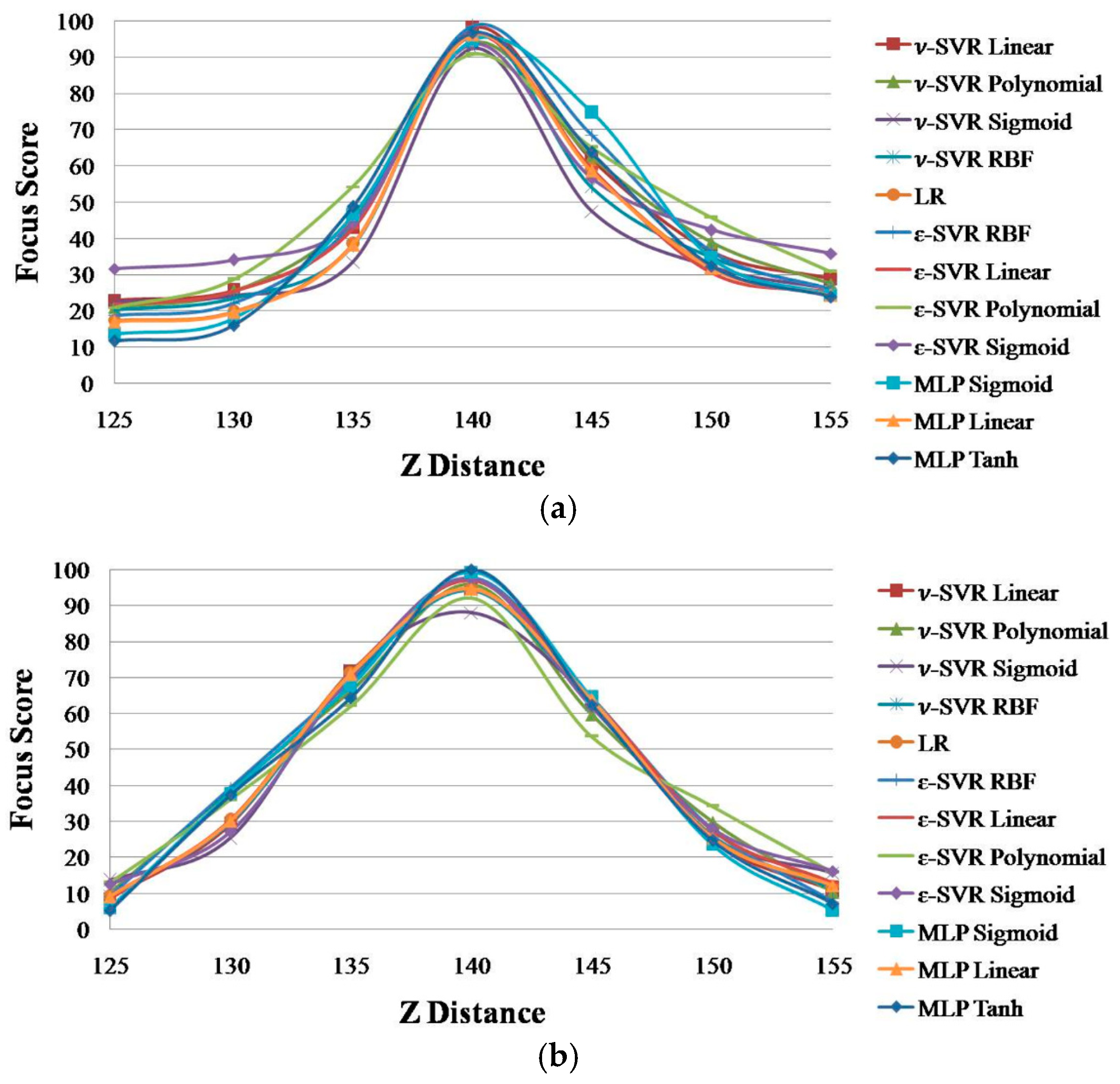
Figure 12.
The focus score graphs of the proposed method and the four individual methods of focus measurement. (a) Database 1; (b) Database 2.
Figure 12.
The focus score graphs of the proposed method and the four individual methods of focus measurement. (a) Database 1; (b) Database 2.
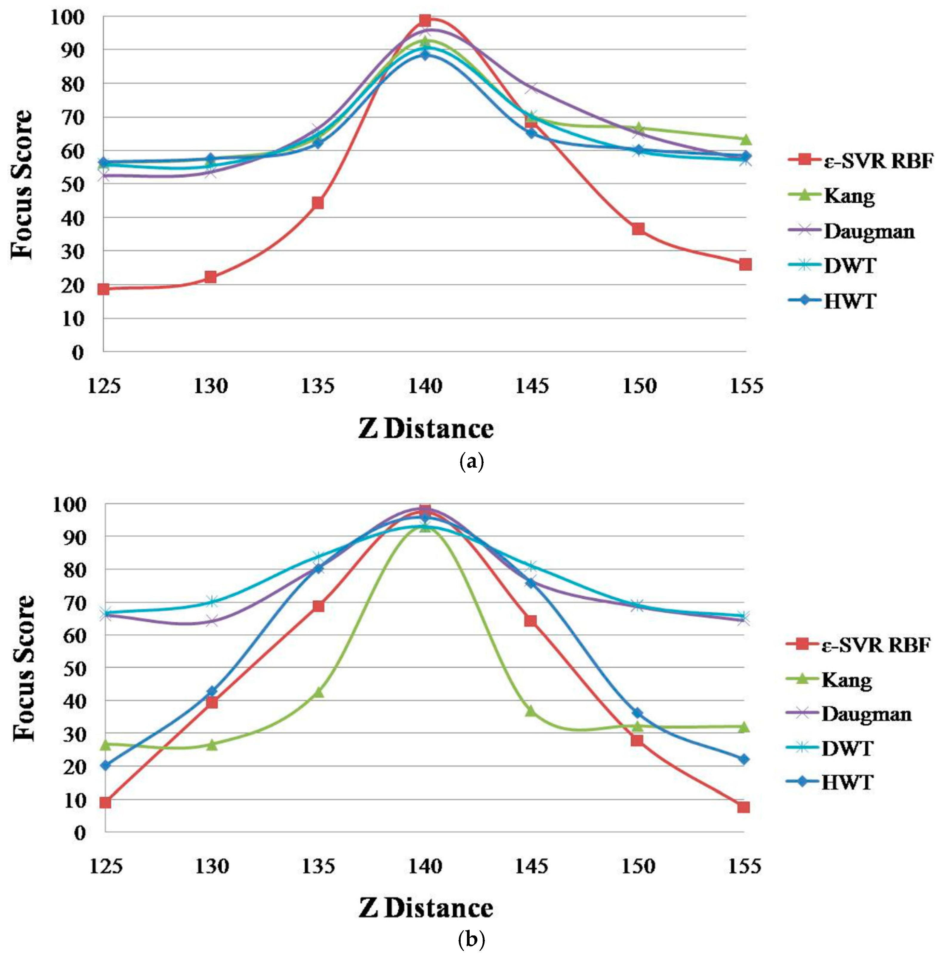
Figure 13.
Experiment for getting the ground-truth Z distance by the Patriot device.


Table 1.
Comparison of focus assessment methods.
| Category | Focus Measurements in Spatial Domain | Focus Measurements in Wavelet Domain | Hybrid Method (Proposed Method) |
|---|---|---|---|
| Method |
|
| The proposed method is a combination of the spatial and wavelet methods using ε-SVR |
| Advantages |
|
| Higher accuracy of focus assessment compared to the spatial or wavelet domain methods |
| Disadvantages |
|
| - Training procedure is required |
Table 2.
The average difference between focus scores of daytime and nighttime images: before and after using linear normalization.
Table 2.
The average difference between focus scores of daytime and nighttime images: before and after using linear normalization.
| Methods | Database 1 | Database 2 | ||
|---|---|---|---|---|
| Before linear Normalization | After Linear Normalization | Before Linear Normalization | After Linear Normalization | |
| Daugman [9] | 4.08 | 3.43 | 2.99 | 2.51 |
| Kang [10] | 4.81 | 3.93 | 3.78 | 1.95 |
| DWT [11] | 1.97 | 1.93 | 0.32 | 0.18 |
| HWT [18] | 5.98 | 4.78 | 2.16 | 0.86 |
Table 3.
Average performance evaluation ratio (PER) (standard deviation) of four spatial domain methods and two wavelet domain methods.
Table 3.
Average performance evaluation ratio (PER) (standard deviation) of four spatial domain methods and two wavelet domain methods.
| Method | Database 1 | Database 2 |
|---|---|---|
| Daugman [9] | 0.25 (0.031) | −0.0007 (0.029) |
| Entropy [13] | 0.37 (0.027) | 0.16 (0.03) |
| Kang [10] | 0.18 (0.025) | 0.13 (0.026) |
| LoG [12] | 0.35 (0.028) | 0.24 (0.029) |
| DWT [11] | 0.05 (0.025) | −0.09 (0.03) |
| HWT [18] | 0.08 (0.026) | −0.15 (0.025) |
Table 4.
Average PER (standard deviation) values of ε-SVR, ν-SVR, LR and MLP using different kernels with the two databases.
Table 4.
Average PER (standard deviation) values of ε-SVR, ν-SVR, LR and MLP using different kernels with the two databases.
| Method | Kernel | Database 1 | Database 2 |
|---|---|---|---|
| ν-SVR | Linear | 0.0399 (0.029) | −0.2492 (0.03) |
| Polynomial | 0.0434 (0.028) | −0.3036 (0.031) | |
| Sigmoid | 0.0971 (0.026) | −0.0649 (0.029) | |
| RBF | 0.0382 (0.027) | −0.2667 (0.032) | |
| LR | 0.0186 (0.031) | −0.2381 (0.028) | |
| ε-SVR | Linear | 0.0654 (0.03) | −0.2568 (0.027) |
| Polynomial | 0.0382 (0.025) | −0.1798 (0.029) | |
| Sigmoid | 0.1462 (0.028) | −0.2095 (0.027) | |
| RBF | 0.0002 (0.025) | −0.3531 (0.026) | |
| MLP | Linear | 0.0185 (0.028) | −0.2392 (0.029) |
| Sigmoid | 0.0788 (0.029) | −0.3528 (0.03) | |
| Tanh | 0.2286 (0.03) | −0.1530 (0.031) | |
Table 5.
Average PER (standard deviation) values of the proposed method and the four individual methods of the focus measurement with the two databases.
Table 5.
Average PER (standard deviation) values of the proposed method and the four individual methods of the focus measurement with the two databases.
| Method | Database 1 | Database 2 | Average |
|---|---|---|---|
| Daugman [9] | 0.25 (0.031) | −0.0007 (0.029) | 0.12465 (0.03) |
| Kang [10] | 0.18 (0.025) | 0.13 (0.026) | 0.155 (0.026) |
| DWT [11] | 0.05 (0.025) | −0.09 (0.03) | −0.02 (0.028) |
| HWT [18] | 0.08 (0.026) | −0.15 (0.025) | −0.035 (0.026) |
| Proposed method | 0.0002 (0.025) | −0.3531 (0.026) | −0.17645 (0.026) |
Table 6.
Comparisons on MAEs of Z distance estimation by our method and previous methods (unit: cm).
© 2017 by the authors. Licensee MDPI, Basel, Switzerland. This article is an open access article distributed under the terms and conditions of the Creative Commons Attribution (CC BY) license (http://creativecommons.org/licenses/by/4.0/).
Share and Cite
MDPI and ACS Style
Luong, D.T.; Kang, J.S.; Nguyen, P.H.; Lee, M.B.; Park, K.R. Focus Assessment Method of Gaze Tracking Camera Based on ε-Support Vector Regression. Symmetry 2017, 9, 86. https://doi.org/10.3390/sym9060086
AMA Style
Luong DT, Kang JS, Nguyen PH, Lee MB, Park KR. Focus Assessment Method of Gaze Tracking Camera Based on ε-Support Vector Regression. Symmetry. 2017; 9(6):86. https://doi.org/10.3390/sym9060086
Chicago/Turabian StyleLuong, Duc Thien, Jeon Seong Kang, Phong Ha Nguyen, Min Beom Lee, and Kang Ryoung Park. 2017. "Focus Assessment Method of Gaze Tracking Camera Based on ε-Support Vector Regression" Symmetry 9, no. 6: 86. https://doi.org/10.3390/sym9060086
Note that from the first issue of 2016, this journal uses article numbers instead of page numbers. See further details here.