Granular Structure of Type-2 Fuzzy Rough Sets over Two Universes

1
School of Computer and Information Technology, Shanxi University, Taiyuan 030006, Shanxi, China
2
School of Science, North University of China, Taiyuan 030051, Shanxi, China
*
Author to whom correspondence should be addressed.
Symmetry 2017, 9(11), 284; https://doi.org/10.3390/sym9110284
Submission received: 24 October 2017
/
Revised: 14 November 2017
/
Accepted: 15 November 2017
/
Published: 21 November 2017
(This article belongs to the Special Issue Fuzzy Sets Theory and Its Applications)
Abstract
:Granular structure plays a very important role in the model construction, theoretical analysis and algorithm design of a granular computing method. The granular structures of classical rough sets and fuzzy rough sets have been proven to be clear. In classical rough set theory, equivalence classes are basic granules, and the lower and upper approximations of a set can be computed by those basic granules. In the theory of fuzzy rough set, granular fuzzy sets can be used to describe the lower and upper approximations of a fuzzy set. This paper discusses the granular structure of type-2 fuzzy rough sets over two universes. Definitions of type-2 fuzzy rough sets over two universes are given based on a wavy-slice representation of type-2 fuzzy sets. Two granular type-2 fuzzy sets are deduced and then proven to be basic granules of type-2 fuzzy rough sets over two universes. Then, the properties of lower and upper approximation operators and these two granular type-2 fuzzy sets are investigated. At last, several examples are given to show the applications of type-2 fuzzy rough sets over two universes.
1. Introduction
According to Chen et al., granular computing is a general computing theory for using granules such as classes, clusters, subsets, groups and intervals to build an efficient computational model for complex applications with huge amounts of data, information and knowledge [1].
Rough set theory [2], proposed by Pawlak in 1982, can be used to reveal and express knowledge hidden in information systems in the form of decision rules by the concepts of lower and upper approximations. Here, equivalence classes are used as the basic granules to express the lower and upper approximations. Taken in this sense, rough set theory is a granular computing method.
Traditional rough set theory only manipulated decision systems with symbolic attribute values, whereas in some real-world applications, the values of attributes could be both symbolic and real-valued. In 1990, Dubois and Prade [3] proposed the definition of fuzzy rough sets by combining fuzzy sets and rough sets, then many studies were carried out in the field of fuzzy rough sets [4,5,6,7,8,9,10,11,12,13,14]. In [15], fuzzy rough sets were applied to feature selection for the first time. Wu et al. studied the generalized fuzzy rough sets using both constructive and axiomatic approaches [16,17]. Mi and Zhang [18] introduced the definitions of generalized fuzzy lower and upper approximation operators determined by a residual implication and studied the composition of two approximation spaces. Yeung et al. [19] studied the lattice and topological structures of fuzzy rough sets. Chen et al. discussed the granular structure of fuzzy rough sets and developed a theory of granular computing based on fuzzy relations in [20]. They proposed the concept of granular fuzzy sets and investigated the properties of these sets using constructive and axiomatic approaches. The granular fuzzy sets were used to describe the lower and upper approximations of a fuzzy set within the framework of granular computing, and the structure of attribute reduction in terms of granular fuzzy sets was characterized.
Type-2 fuzzy rough set is a combination of rough sets and type-2 fuzzy sets. As an extension of fuzzy sets, type-2 fuzzy sets [21] are useful in circumstances where it is difficult to determine the exact membership functions of a fuzzy set because the membership degrees are fuzzy themselves. Type-2 fuzzy rough sets may solve problems with higher complexity, and there have been several literature works in this field [22,23,24]. In some practical applications, we often encounter situations involving more than one universe. For example, in medical diagnosis, a certain disease may simultaneously have several symptoms, whereas one symptom may be shared by different diseases. Zhang et al. [25] proposed a general study of interval-valued fuzzy rough sets on two universes of discourse. Sun et al. [26] defined the fuzzy compatible relation and presented the fuzzy rough set model on the different universes. Liu et al. proposed the graded rough set model on two distinct, but related universes in [27]. Ma et al. [28] presented the properties of the probabilistic rough set over two universes and discussed the uncertainty measure of the knowledge granularity and rough entropy for a probabilistic rough set over two universes. Sun et al. [29] considered a problem of emergency material demand prediction based on a fuzzy rough set model over two universes. Yang et al. proposed a fuzzy probabilistic rough set model on two universes and presented concepts of the inverse lower and upper approximation operators in [30]. However, type-2 fuzzy rough sets over two universes have not been discussed.
As generalizations of rough sets, type-2 fuzzy rough sets over one or two universes can be incorporated into the scope of granular computing if we can reveal their granular structures, and the granular structures will be beneficial to their application. In [24], we generalized the concepts of granular fuzzy sets in [20] to the frame of type-2 fuzzy sets and presented a definition of granular type-2 fuzzy sets without proof of its reasonability. Then, we discussed the granular structure of type-2 fuzzy rough sets over one universe based on these two granular type-2 fuzzy sets.
In this paper, the granular structure discussed in [24] will be generalized to the type-2 fuzzy rough sets over different universes based on novel granular type-2 fuzzy sets, which are deduced from the definition of type-2 fuzzy rough sets, and consequently, more reasonable than those given in [24]. The rest of this paper is organized as follows. Fundamental concepts and properties that will be used in this paper are reviewed in Section 2. Section 3 introduces the definition of a type-2 fuzzy rough set over two universes. In Section 4, the granular structure of type-2 fuzzy rough sets over two universes is discussed using granular type-2 fuzzy sets. Some illustrative examples are given in Section 5, and conclusions are presented in Section 6.
2. Preliminaries
2.1. Type-2 Fuzzy Sets
To facilitate the discussion, we introduce the basic definitions and properties of type-2 fuzzy sets in this section with reference to [31,32].
For a nonempty universe X, a type-2 fuzzy set on X can be characterized by a type-2 membership function , i.e.,
or
where and denotes union over all admissible x and u. denotes the class of all type-2 fuzzy sets on the universe X.
For a given , is a fuzzy set on , which is called a vertical slice of or a secondary membership function, and it can be denoted by or . is called the primary membership of . The amplitude of a secondary membership function is called a secondary grade. A vertical-slice representation of a type-2 fuzzy set is:
Mendel and John [32] presented a wavy-slice representation for discrete type-2 fuzzy sets (both X and are assumed to be discrete) in 2002. Suppose that X is discretized into N values, and that at each of these values, is discretized into values, i.e.,
For a discrete type-2 fuzzy set , take exactly one element from , , , namely , , , each with its associated secondary grade, namely , , , then we get a wavy-slice of , i.e.,
which is called an embedded type-2 set. An embedded type-1 set is the union of all the primary memberships of set , i.e.,
The total of is and so is that of .
The Representation Theorem [32] (the wavy-slice representation of a type-2 fuzzy set) proposed by Mendel and John indicates that a discrete type-2 fuzzy set can be represented as the union of its embedded type-2 sets, i.e.,
where
Consider two discrete type-2 fuzzy sets and , which are expressed by their embedded type-2 sets:
and:
the operations of union, intersection and complement are defined as follows:
The expressions for , and can be obtained as:
where and indicate the join and meet of the secondary membership functions and , and indicates the negation of the secondary membership function .
Considering two discrete type-2 fuzzy sets and , which have unique embedded type-2 sets, i.e.,
then is defined as and
For a family of discrete type-2 fuzzy sets with unique embedded type-2 sets:
where is a finite index set, the union of these type-2 fuzzy sets is:
and the intersection of these type-2 fuzzy sets is:
Obviously, and if .
Let X and Y be two nonempty universes. A type-2 fuzzy relation from X to Y is a type-2 fuzzy set . If , then is called a type-2 fuzzy relation on X.
A discrete type-2 fuzzy relation can be represented as the union of its embedded type-2 sets:
where (), and is the l-th embedded type-2 set of .
2.2. Fuzzy Rough Sets
In 1982, Pawlak proposed the theory of rough set as a new mathematical tool for reasoning about data. For a finite and nonempty universe X, if is an equivalence relation on X, i.e., R is reflexive, symmetric and transitive, the pair is called an approximation space. For any , is called the equivalence class containing x. The family of all equivalence classes defines a partition of the universe X. Two elements x and y are said to be indiscernible if they belong to the same equivalence class. Given an arbitrary set it may be characterized by a pair of lower and upper approximations defined as:
or:
That is to say, equivalence classes can be used as basic granules to approximate a set.
Let X be a nonempty universe and R be a fuzzy binary relation on X. The fuzzy rough set of a fuzzy set A is a pair such that for every
Chen et al. [20] discovered the granular structure of fuzzy rough sets and pointed out that fuzzy sets and were basic granules corresponding to the equivalence classes, which were defined as:
where is a fuzzy point, T is a triangular norm, S is a triangular conorm, N is a negator and T and S are dual with respect to N. For a T-fuzzy similarity relation R, the lower and upper approximations of a fuzzy set A can be expressed as the union or intersection of some basic fuzzy information granules:
3. Type-2 Fuzzy Rough Sets over Two Universes
Since type-2 fuzzy sets can be used to describe more uncertainties than type-1 fuzzy sets because the membership functions of type-2 fuzzy sets are themselves fuzzy, type-2 fuzzy rough sets can be used to solve problems with more uncertainties. In this section, we will extend the definition of type-2 fuzzy rough set proposed in [24], which was defined on one universe, to the circumstance of two different universes.
Definition 1.
Let X and Y be two nonempty finite universes and be a type-2 fuzzy relation from X to Y. The triple set is called a type-2 fuzzy approximation space over two different universes. For any type-2 fuzzy set , the lower approximation and the upper approximation of with respect to are two type-2 fuzzy sets in X, respectively. If and can be represented as by the representation theorem, we have:
where and are the embedded type-2 set and embedded type-1 set of , respectively, and is the simplified notation of , whereas and are the embedded type-2 and embedded type-1 set of , respectively, and is the simplified notation of .
Consequently, and can be calculated by:
and
The ordered pair is called a type-2 fuzzy rough set over two universes.
Note: If and degenerate to be interval type-2 fuzzy sets,
and:
If and degenerate to be type-1 fuzzy sets, then:
which are in accordance with the definition of (type-1) fuzzy rough set over two universes given in [29].
Example 1.
Let , . Suppose is a type-2 fuzzy relation from X to Y, which can be defined as follows:
Then, , where and are embedded type-2 sets of :
Next, we will discuss the properties of the lower and upper approximation operators.
Lemma 1.
Let X and Y be two nonempty finite universes and be a type-2 fuzzy relation from X to Y. For any , if are embedded type-2 sets of and respectively, the following properties hold:
- 1.
- ;
- 2.
- ;
- 3.
- ;
- 4.
- .
Proof.
- For any
- For any
- For any
- For any
☐
Theorem 1.
Let X and Y be two nonempty finite universes and be a type-2 fuzzy relation from X to Y. For any , the following properties hold:
- 1.
- ;
- 2.
- ;
- 3.
- ;
- 4.
- .
Proof.
- 1.
- 2.
- 3.
- 4.
☐
4. Granular Structure of Type-2 Fuzzy Rough Sets over Two Universes
The granular structures of classical rough sets and ordinary fuzzy rough sets are clear, and the lower and upper approximation sets can be represented by some basic granules. Here, we will discuss the basic granules in type-2 fuzzy rough sets over two universes, which can be used to calculate the lower and upper approximation sets of a type-2 fuzzy set.
In classical rough set theory, for a nonempty and finite universe X and an equivalent relation , the upper and lower approximation sets of can be defined as follows:
Take and in the above two equations respectively, and we have:
Next, we will try to find the “equivalence classes” of a type-2 fuzzy point and its complement, both of which should be type-2 fuzzy sets.
Let Y be a nonempty universes. A type-2 fuzzy point in Y is a special type-2 fuzzy set defined as follows: for any ,
where and . The complement of , denoted by , is also a type-2 fuzzy set on Y: for any ,
Definition 2.
Let X and Y be two nonempty finite universes. Suppose is a type-2 fuzzy relation from X to Y, is an embedded type-2 set of and is the corresponding embedded type-1 set. For a type-2 fuzzy point , two granular type-2 fuzzy sets and are defined as: for any
and
Let ,
From the above definition, it is clear that and .
Example 2.
Consider the type-2 fuzzy relation given in the previous example. Take a type-2 fuzzy point by
we have
so:
By:
we have:
so:
and are depicted in Figure 2. Obviously, is exactly the complement of .
Theorem 2.
Let X and Y be two nonempty finite universes and be a type-2 fuzzy relation from X to Y. If is an embedded type-2 set of and is the corresponding embedded type-1 set, for we have:
- 1.
- 2.
- 3.
- 4.
Proof.
- For any ,
- For any ,
- For any ,
- For any ,
☐
Theorem 3.
Let X and Y be two nonempty finite universes. Suppose and are type-2 fuzzy relations from X to Y and and are embedded type-2 sets of and , respectively, then for
- 1.
- 2.
- 3.
- 4.
Proof.
- For any ,
- For any ,
- For any ,
- For any ,
☐
Lemma 2.
Let X and Y be two nonempty finite universes. Suppose is a type-2 fuzzy relation from X to Y, is an embedded type-2 set of and is the corresponding embedded type-1 set. For
- 1.
- If
- 2.
- If
Proof.
Obviously. ☐
Theorem 4.
Let be a discrete type-2 fuzzy relation from X to Y, where X and Y are nonempty finite universes. For a discrete type-2 fuzzy set , if and are embedded type-2 sets of and respectively, we have:
and:
Proof.
For any ,
☐
We have mentioned in Section 2.2 that basic granules in the theory of the classic rough set are equivalence classes, and the lower and upper approximations of a crisp set can be computed by the basic granules or the complements of the basic granules. Similarly, in the theory of fuzzy rough set, Chen et al. [20] proved that and , which are called basic granules of fuzzy rough sets, corresponded to the equivalence classes and the complements of equivalence classes, respectively, and the upper and lower approximations of a fuzzy set can be expressed as the union or intersection of basic granules. Taking and as basic granule sets, the above theorem reveals that these basic granules can be used to compute the upper and lower approximations of a type-2 fuzzy set by the operators of union and intersection. Therefore, and correspond to the equivalence classes and the complements of equivalence classes, respectively.
Example 3.
Similar to the previous example, we can calculate granular type-2 fuzzy sets of for any :
5. Examples
Example 4.
Suppose is a set of four different houses, all of which can be described by an attribute set where stands for , stands for , stands for , stands for and stands for .
The correlation degree between X and Y (i.e., ) is given in Table 1.
Suppose is a client who wants to purchase a house among the four alternative offers, and the demand of can be described by a type-2 fuzzy set (Figure 3a):
By the definitions of the lower and upper type-2 fuzzy rough approximation operators, we can calculate the lower and upper type-2 fuzzy rough approximations of .
Since and , where:
we have:
and:
Thus,
From
we have:
Consequently (Figure 3b),
Let:
where is the centroid of .
If , then is the best choice of
If , then consider : if , we have that is the best choice of if , we take as the best choice of [29].
Since , , , is the best house for .
From the definition of , it is clear that client pays most attention to and , the surrounding facilities and the structure, and , price, is the least important factor. is the best house both in surrounding facilities and structure.
Consider another client for house purchasing (Figure 4a):
Take:
and:
Using the definition of granular type-2 fuzzy sets, we can compute the upper and lower approximations of :
where:
and:
Then, we have:
and:
From:
we have:
Consequently (Figure 4b),
Since , , , is the best house for .
For client , the most important factors are and , the price and the structure; the least important factor is , the greening. The above method considered all the requirements of the client: the choice is of good behavior in and ; whereas, and are affordable, but not well structured. Figure 4a depicts the demand of , and Figure 4b depicts and . It can be seen from Figure 4b that the memberships of are largest in both and . That is to say, is the best choice of client .
Example 5.
We use an emergency decision-making problem to illustrate the application of type-2 fuzzy rough sets over two universes. Since emergency management is closely related to social stability and economic development, many studies have been conducted on it. In this example, we use the granular type-2 fuzzy sets of type-2 fuzzy rough sets to analyze such a problem and compare it to the model of fuzzy rough set on probabilistic approximation space over two universes proposed by Sun et al. in [33].
Unconventional emergency events, such as tornadoes, typhoons, earthquakes and floods, often occur unexpectedly, and the severity and extent of the impact are difficult to describe precisely. Approaches to handling uncertainty and incomplete data and information can be used to study the emergency decision-making problem.
Sun et al. [33] investigated the application of fuzzy rough set on probabilistic approximation space over two universes by an emergency decision-making problem. In order to compare with their method, we use a similar example in this section with some data modified.
Consider an emergency decision-making problem during an earthquake and suppose that the area affected can be divided into several different disaster areas according to the administrative district or the distribution of geography. We use to denote the set of disaster areas. The general characteristic factors that are used to describe the emergency event are denoted by , where stands for Affected population, stands for Economic loss, stands for Risk of occurrence of a new disaster, stands for Damage to transportation, stands for Number of destroyed facilities, stands for Possibility of a disease outbreak and stands for Weather conditions. The degree of the relationship between these characteristic factors and the disaster areas is available based on history records about past earthquakes. For the convenience of comparison, we use the data given in [33], which are presented in Table 2. The larger the value of , the more important the characteristic for the area . For example, implies that more population is affected in area than in .
In [33], is the fuzzy description of all the characteristic factors, and the conclusion is: (1) , and are the most seriously affected areas, which need immediate rescue; (2) does not need rescue immediately; (3) the situation of and cannot be decided because of insufficient information.
Since we cannot acquire accurate and sufficient information immediately after the earthquake, if the exact memberships for those characteristic factors are unavailable, the information collected after a new earthquake can be described by a type-2 fuzzy set on Y:
By the wavy-slice representation of a type-2 fuzzy set,
where:
Then, we present a procedure for the emergency decision-making problem based on the granular type-2 fuzzy sets of type-2 fuzzy rough sets over two universes.
- Step 1.
- Computing all the granular type-2 fuzzy sets , (; ) (Table 3);
- Step 2.
- Computing for (Table 4);
- Step 3.
- Computing (Table 5);
- Step 4.
- Computing all the granular type-2 fuzzy sets , (; ) (Table 6);
- Step 5.
- Computing for (Table 7);
- Step 6.
- Computing (Table 8);
- Step 7.
- Computing sum of and (Table 9);
- Step 8.
- Making the decision according to:where C is the centroid of fuzzy sets. If , then is the most seriously affected areas. If , then consider : if , we have is the most seriously affected areas; if , we take as the most seriously affected areas [29].
Since , , , is the most seriously affected area, which needs to be rescued immediately. Since , is the least seriously affected area.
In Table 3, the maximums for every granular type-2 fuzzy sets have been highlighted in bold. We have the following conclusion:
- 1.
- Considering characteristic factor , all the areas are equally serious;
- 2.
- Considering characteristic factor , area and area are more serious;
- 3.
- Considering characteristic factor , area and area are more serious;
- 4.
- Considering characteristic factor , area and area are more serious;
- 5.
- Considering characteristic factor , area is more serious;
- 6.
- Considering characteristic factor , area and area are more serious;
- 7.
- Considering characteristic factor , area is more serious;
- 8.
- Area is serious in the aspect of (risk of occurrence of a new disaster) and (weather conditions);
- 9.
- Area is the least serious area.
Consider another type-2 fuzzy description for an earthquake:
By the wavy-slice representation of type-2 fuzzy sets, can be represented as , where:
Similar to the above procedure, we should compute , , , and the computation process is presented in the following tables (Table 10, Table 11, Table 12, Table 13, Table 14, Table 15 and Table 16):
In Table 10, the maximums for every granular type-2 fuzzy sets have been highlighted in bold. We have the following conclusion:
- 1.
- Considering characteristic factor , is more serious;
- 2.
- Considering characteristic factor , is the least serious area;
- 3.
- Considering characteristic factor , and are more serious;
- 4.
- Considering characteristic factor , is more serious;
- 5.
- Considering characteristic factor , is more serious;
- 6.
- Considering characteristic factor , is more serious;
- 7.
- Considering characteristic factor , all the areas are equally serious;
- 8.
- Area is serious in the respect of (affected population) and (economic loss).
Since , is the most seriously affected area and needs immediate rescue.
In [33], the description of an earthquake is a fuzzy set:
that is to say, exact memberships of the characteristic factors have been decided by the information acquired after the earthquake. However, if the information is insufficient and the memberships of some factors cannot be decided, we have to take fuzzy sets as membership functions of those factors. In this example, we consider such conditions and use type-2 fuzzy sets as the descriptions of emergency events:
and:
A reasonable decision-making process for the unconventional emergency event has been made using the type-2 fuzzy rough sets over two universes. For the type-2 fuzzy description , whose secondary membership functions are equal to or close to the corresponding memberships of the fuzzy description A, the decision is similar to that of [33], whereas for the type-2 fuzzy description , whose secondary membership functions are equal to or close to the corresponding memberships of the complement of A, i.e., an almost opposite conclusion has been made. Furthermore, the granular type-2 fuzzy sets make it possible to analyze the problem from each aspect.
6. Conclusions
Rough set theory is a method of granular computing, and equivalence classes are basic granules that can be used to approximate a set. Whether the granular structure of type-2 fuzzy rough sets over two universes is as clear as that of classical rough sets is what the authors want to discuss. At first, the definition of a type-2 fuzzy rough set over two different universes is proposed based on a general type-2 fuzzy relation from one universe to another, and the lower and upper approximations of a type-2 fuzzy set are defined in terms of membership functions. Then, two granular type-2 fuzzy sets are defined for an arbitrary type-2 fuzzy point, which are proven to be analogous to equivalence classes and complements of equivalence classes of rough sets respectively, since they can be used to express the upper and lower approximations of a type-2 fuzzy set by the operators union and intersection. Therefore, these granular type-2 fuzzy sets are the basic granules of type-2 fuzzy rough sets and can be considered to be type-2 fuzzy equivalence classes and complements of type-2 fuzzy equivalence classes of a type-2 fuzzy point. The authors discussed the properties of the upper and lower type-2 fuzzy rough approximation operators and the granular type-2 fuzzy sets. Two illustrative examples showed some simple applications of the model proposed in this paper. Future work by the authors will consider the practical application of the granular structure of type-2 fuzzy rough sets over two universes.
Acknowledgments
The authors would like to thank the anonymous referees for their valuable comments and suggestions, which have significantly improved the quality and presentation of this paper. The works described in this paper are supported by the National Natural Science Foundation of China (Nos. 61672331, 61573231, U1435212 and 61432011) and Shanxi Science and Technology Infrastructure (2015091001-0102).
Author Contributions
Juan Lu is the principal investigator of this work, and she wrote this manuscript. De-Yu Li provided some important suggestions and checked the whole manuscript. Yan-Hui Zhai and He-Xiang Bai provided several suggestions for improving the quality of this manuscript. All authors revised and approved the publication.
Conflicts of Interest
The authors declare no conflict of interest.
References
- Chen, C.P.; Zhang, C.Y. Data-intensive applications, challenges, techniques and technologies: A survey on Big Data. Inf. Sci. 2014, 275, 314–347. [Google Scholar] [CrossRef]
- Pawlak, Z. Rough sets. Int. J. Comput. Inf. Sci. 1982, 11, 341–356. [Google Scholar] [CrossRef]
- Dubois, D.; Prade, H. Rough fuzzy sets and fuzzy rough sets. Int. J. Gen. Syst. 1990, 17, 191–209. [Google Scholar] [CrossRef]
- Radzikowska, A.M.; Kerre, E.E. A comparative study of fuzzy rough sets. Fuzzy Sets Syst. 2002, 126, 137–155. [Google Scholar] [CrossRef]
- Deng, T.Q.; Chen, Y.M.; Xu, W.L.; Dai, Q.H. A novel approach to fuzzy rough sets based on a fuzzy covering. Inf. Sci. 2007, 177, 2308–2326. [Google Scholar] [CrossRef]
- Liu, G.L. Using one axiom to characterize rough set and fuzzy rough set approximations. Inf. Sci. 2013, 223, 285–296. [Google Scholar] [CrossRef]
- Chen, D.G.; Zhang, L.; Zhao, S.Y.; Hu, Q.H.; Zhu, P.F. A Novel Algorithm for Finding Reducts with Fuzzy Rough Sets. IEEE Trans. Fuzzy Syst. 2012, 20, 385–389. [Google Scholar] [CrossRef]
- Dai, J.H.; Xu, Q. Attribute selection based on information gain ratio in fuzzy rough set theory with application to tumor classification. Appl. Soft Comput. 2013, 13, 211–221. [Google Scholar] [CrossRef]
- Parthaláin, N.M.; Jensen, R. Unsupervised fuzzy-rough set-based dimensionality reduction. Inf. Sci. 2013, 229, 106–121. [Google Scholar] [CrossRef]
- Chen, D.G.; Kwong, S.; He, Q.; Wang, H. Geometrical interpretation and applications of membership functions with fuzzy rough sets. Fuzzy Sets Syst. 2012, 193, 122–135. [Google Scholar] [CrossRef]
- Hu, Q.H.; Zhang, L.; An, S.; Zhang, D.; Yu, D. On Robust Fuzzy Rough Set Models. IEEE Trans. Fuzzy Syst. 2012, 20, 636–651. [Google Scholar] [CrossRef]
- Tiwari, S.P.; Srivastava, A.K. Fuzzy rough sets, fuzzy preorders and fuzzy topologies. Fuzzy Sets Syst. 2013, 210, 63–68. [Google Scholar] [CrossRef]
- El-Latif, A.A.A.; Ramadan, A.A. On L-Double Fuzzy rough sets. Iran. J. Fuzzy Syst. 2016, 13, 125–142. [Google Scholar]
- Morsi, N.N.; Yakout, M.M. Axiomatics for fuzzy rough sets. Fuzzy Sets Syst. 1998, 100, 327–342. [Google Scholar] [CrossRef]
- Ludmila, K. Fuzzy rough sets: Application to features selection. Fuzzy Sets Syst. 1992, 51, 147–153. [Google Scholar]
- Wu, W.Z.; Mi, J.S.; Zhang, W.X. Generalized fuzzy rough sets. Inf. Sci. 2003, 151, 263–282. [Google Scholar] [CrossRef]
- Wu, W.Z.; Zhang, W.X. Constructive and axiomatic approaches of fuzzy approximation operators. Inf. Sci. 2004, 159, 233–254. [Google Scholar] [CrossRef]
- Mi, J.S.; Zhang, W.X. An axiomatic characterization of a fuzzy generalization of rough sets. Inf. Sci. 2004, 160, 235–249. [Google Scholar] [CrossRef]
- Yeung, D.S.; Chen, D.G.; Tsang, E.C.C.; Lee, J.W.T.; Wang, X.Z. On the Generalization of Fuzzy Rough Sets. IEEE Trans. Fuzzy Syst. 2005, 13, 343–361. [Google Scholar] [CrossRef]
- Chen, D.G.; Yang, Y.P.; Wang, H. Granular computing based on fuzzy similarity relations. Soft Comput. 2011, 15, 1161–1172. [Google Scholar]
- Zadeh, L.A. The concept of a linguistic variable and its application to approximate reasoning-1. Inf. Sci. 1975, 8, 199–249. [Google Scholar] [CrossRef]
- Wang, C.Y. Type-2 fuzzy rough sets based on extended t-norms. Inf. Sci. 2015, 305, 165–183. [Google Scholar] [CrossRef]
- Zhao, T.; Xiao, J. General type-2 fuzzy rough sets based on α-plane Representation theory. Soft Comput. 2014, 18, 227–237. [Google Scholar] [CrossRef]
- Lu, J.; Li, D.Y.; Zhai, Y.H.; Li, H.; Bai, H.X. A model for type-2 fuzzy rough sets. Inf. Sci. 2016, 328, 359–377. [Google Scholar] [CrossRef]
- Zhang, H.Y.; Zhang, W.X.; Wu, W.Z. On characterization of generalized interval-valued fuzzy rough sets on two universes of discourse. Int. J. Approx. Reason. 2009, 51, 56–70. [Google Scholar] [CrossRef]
- Sun, B.Z.; Ma, W.M. Fuzzy rough set model on two different universes and its application. Appl. Math. Model. 2011, 35, 1798–1809. [Google Scholar] [CrossRef]
- Liu, C.H.; Miao, D.Q.; Zhang, N. Graded rough set model based on two universes and its properties. Knowl.-Based Syst. 2012, 33, 65–72. [Google Scholar] [CrossRef]
- Ma, W.M.; Sun, B.Z. Probabilistic rough set over two universes and rough entropy. Int. J. Approx. Reason. 2012, 53, 608–619. [Google Scholar] [CrossRef]
- Sun, B.Z.; Ma, W.M.; Zhao, H.Y. A fuzzy rough set approach to emergency material demand prediction over two universes. Appl. Math. Model. 2013, 37, 7062–7070. [Google Scholar] [CrossRef]
- Yang, H.L.; Liao, X.W.; Wang, S.Y.; Wang, J. Fuzzy probabilistic rough set model on two universes and its applications. Int. J. Approx. Reason. 2013, 54, 1410–1420. [Google Scholar] [CrossRef]
- Mendel, J.M. Advances in type-2 fuzzy sets and systems. Inf. Sci. 2007, 177, 84–110. [Google Scholar] [CrossRef]
- Mendel, J.M.; John, R.I.B. Type-2 fuzzy sets made simple. IEEE Trans. Fuzzy Syst. 2002, 10, 117–127. [Google Scholar] [CrossRef]
- Sun, B.Z.; Ma, W.M.; Chen, X.T. Fuzzy rough set on probabilistic approximation space over two universes and its application to emergency decision-making. Exp. Syst. 2015, 32, 507–521. [Google Scholar] [CrossRef]
Figure 1.
(a) A type-2 fuzzy set , which is defined in Y; (b) the lower approximation and the upper approximation of with respect to , which are type-2 fuzzy sets defined in X. The solid lines depict the upper approximation ; the dotted line depicts the lower approximation .
Figure 1.
(a) A type-2 fuzzy set , which is defined in Y; (b) the lower approximation and the upper approximation of with respect to , which are type-2 fuzzy sets defined in X. The solid lines depict the upper approximation ; the dotted line depicts the lower approximation .

Figure 2.
The solid lines depict and the dotted lines depict .
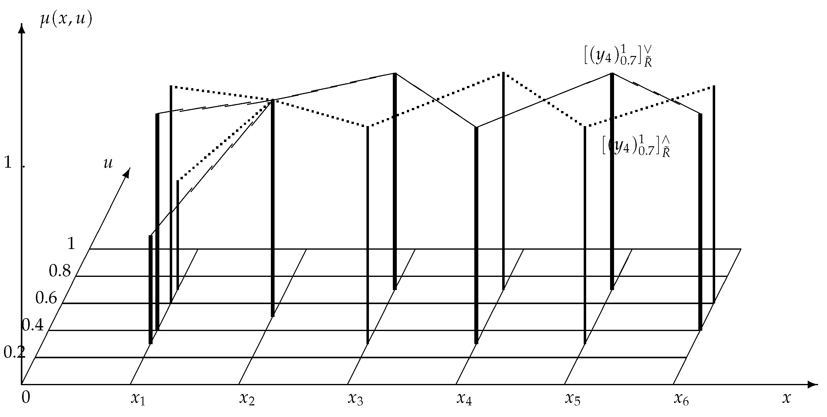
Figure 3.
(a) Demand of client ; (b) the lower approximation and the upper approximation of , which are type-2 fuzzy sets defined in X. The solid line depicts the upper approximation ; the dotted line depicts the lower approximation .
Figure 3.
(a) Demand of client ; (b) the lower approximation and the upper approximation of , which are type-2 fuzzy sets defined in X. The solid line depicts the upper approximation ; the dotted line depicts the lower approximation .

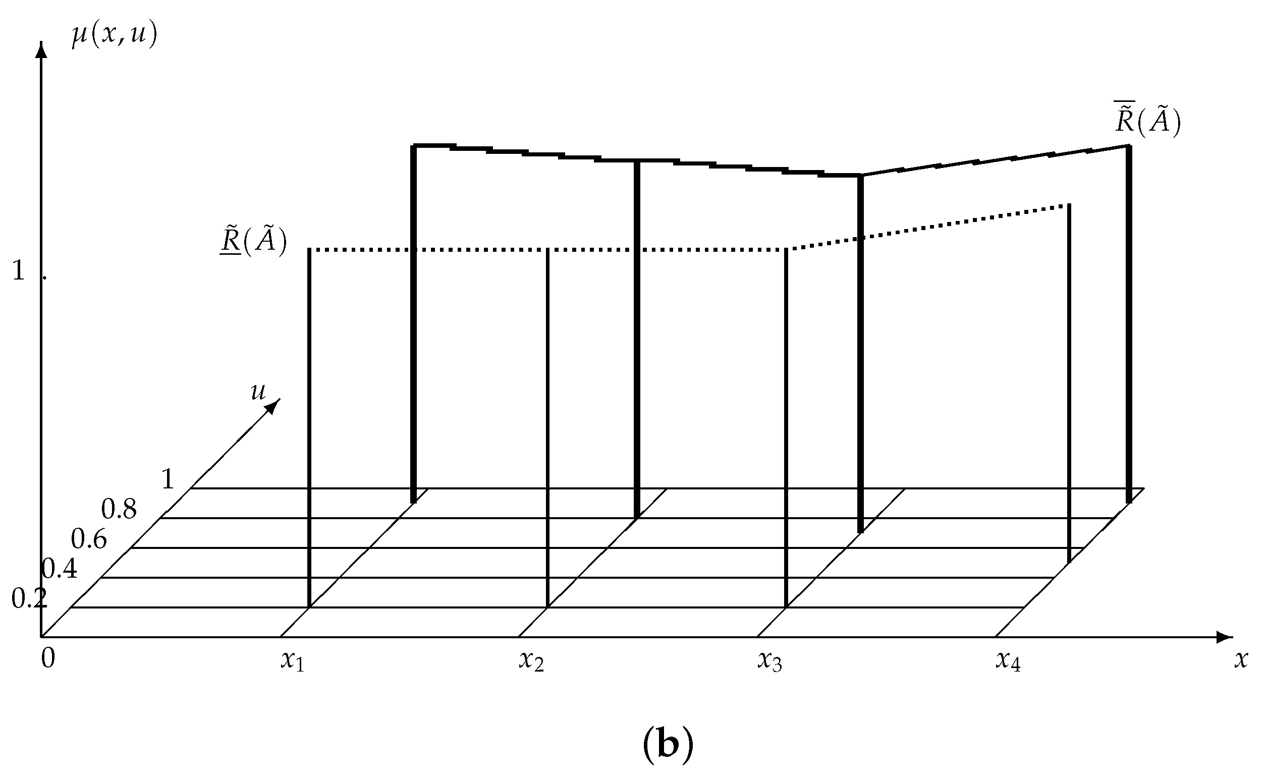
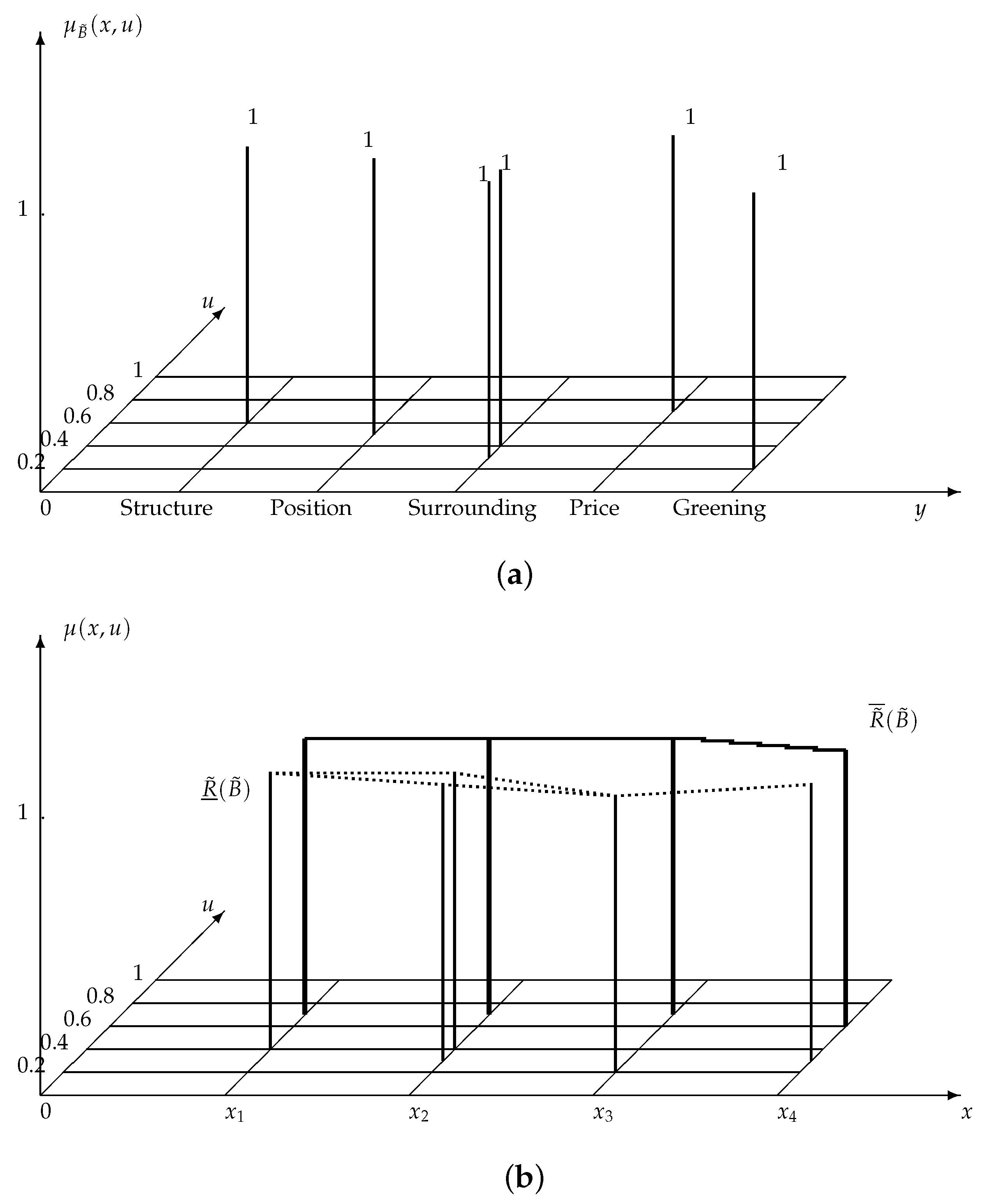
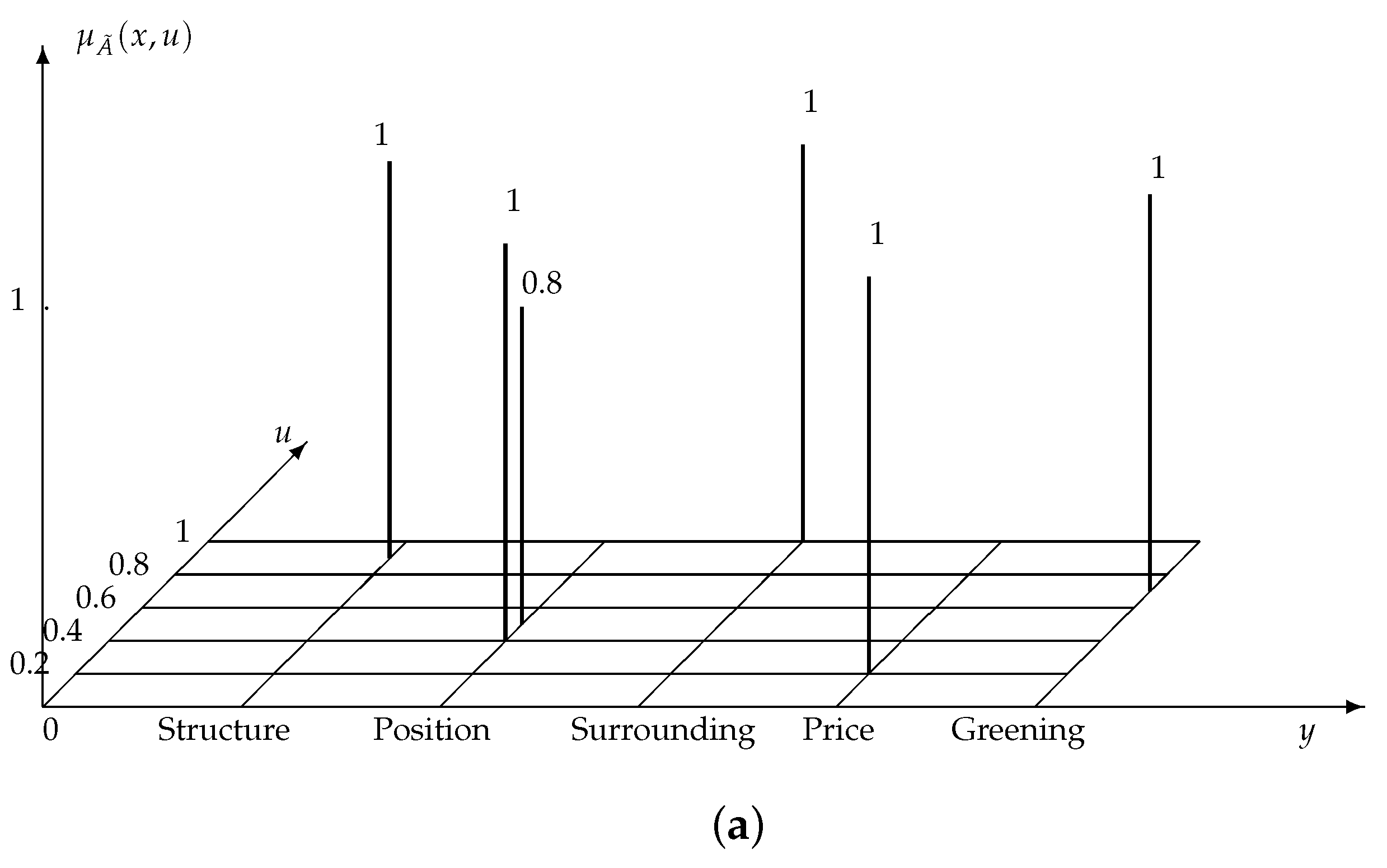
Figure 4.
(a) Demand of client ; (b) the lower approximation and the upper approximation of , which are type-2 fuzzy sets defined in X. The solid line depicts the upper approximation ; the dotted lines depict the lower approximation .
Figure 4.
(a) Demand of client ; (b) the lower approximation and the upper approximation of , which are type-2 fuzzy sets defined in X. The solid line depicts the upper approximation ; the dotted lines depict the lower approximation .

Table 1.
Correlation degree between and .
| 1/1 | 1/0.8 | 1/0.3 + 0.5/0.4 | 1/0.9 | 1/0.6 | |
| 1/0.6 | 1/0.3 | 1/0.8 | 1/1 | 1/0.4 | |
| 1/0.4 | 1/0.6 | 1/0.5 | 1/1 | 1/0.8 | |
| 1/1 | 1/0.5 | 1/0.6 | 1/0.3 | 1/0.7 |
Table 2.
Fuzzy relation R from X to Y.
| 0.3 | 0.1 | 0.4 | 0.4 | 0.1 | 0.1 | 0.5 | |
| 0.3 | 0.3 | 0.5 | 0.1 | 0.3 | 0.1 | 0.5 | |
| 0.4 | 0.3 | 0.5 | 0.1 | 0.3 | 0.1 | 0.6 | |
| 0.7 | 0.4 | 0.2 | 0.1 | 0.2 | 0.1 | 0.3 | |
| 0.2 | 0.5 | 0.2 | 0.3 | 0.5 | 0.5 | 0.4 | |
| 0.3 | 0.5 | 0.2 | 0.2 | 0.2 | 0.3 | 0.3 |
Table 3.
Granular type-2 fuzzy sets .
| 1/0.2 | 1/0.2 | 1/0.2 | 1/0.2 | 1/0.2 | 1/0.2 | |
| 1/0.1 | 1/0.3 | 1/0.3 | 1/0.4 | 1/0.5 | 1/0.5 | |
| 1/0.4 | 1/0.5 | 1/0.5 | 1/0.2 | 1/0.2 | 1/0.2 | |
| 0.8/0.4 | 0.8/0.5 | 0.8/0.5 | 0.8/0.2 | 0.8/0.2 | 0.8/0.2 | |
| 1/0.3 | 1/0.1 | 1/0.1 | 1/0.1 | 1/0.3 | 1/0.2 | |
| 1/0.1 | 1/0.3 | 1/0.3 | 1/0.2 | 1/0.5 | 1/0.2 | |
| 1/0.1 | 1/0.1 | 1/0.1 | 1/0.1 | 1/0.1 | 1/0.1 | |
| 0.5/0.1 | 0.5/0.1 | 0.5/0.1 | 0.5/0.1 | 0.5/0.2 | 0.5/0.2 | |
| 1/0.5 | 1/0.5 | 1/0.6 | 1/0.3 | 1/0.4 | 1/0.3 | |
| 1/0.5 | 1/0.5 | 1/0.6 | 1/0.3 | 1/0.4 | 1/0.3 |
Table 4.
The upper approximations .
| 1/0.5 | 1/0.5 | 1/0.6 | 1/0.4 | 1/0.5 | 1/0.5 | |
| 0.8/0.5 | 0.8/0.5 | 0.8/0.6 | 0.8/0.4 | 0.8/0.5 | 0.8/0.5 | |
| 0.5/0.5 | 0.5/0.5 | 0.5/0.6 | 0.5/0.4 | 0.5/0.5 | 0.5/0.5 | |
| 1/0.5 | 1/0.5 | 1/0.6 | 1/0.4 | 1/0.5 | 1/0.5 | |
| 0.5/0.5 | 0.5/0.5 | 0.5/0.6 | 0.5/0.4 | 0.5/0.5 | 0.5/0.5 | |
| 0.8/0.5 | 0.8/0.5 | 0.8/0.6 | 0.8/0.4 | 0.8/0.5 | 0.8/0.5 | |
| 0.5/0.5 | 0.5/0.5 | 0.5/0.6 | 0.5/0.4 | 0.5/0.5 | 0.5/0.5 | |
| 0.5/0.5 | 0.5/0.5 | 0.5/0.6 | 0.5/0.4 | 0.5/0.5 | 0.5/0.5 |
Table 5.
The upper approximation .
| 1/0.5 | 1/0.5 | 1/0.6 | 1/0.4 | 1/0.5 | 1/0.5 | |
| 0.5 | 0.5 | 0.6 | 0.4 | 0.5 | 0.5 |
Table 6.
Granular type-2 fuzzy sets .
| 1/0.7 | 1/0.7 | 1/0.6 | 1/0.3 | 1/0.8 | 1/0.7 | |
| 1/0.9 | 1/0.8 | 1/0.8 | 1/0.8 | 1/0.8 | 1/0.8 | |
| 1/0.6 | 1/0.5 | 1/0.5 | 1/0.8 | 1/0.8 | 1/0.8 | |
| 0.8/0.6 | 0.8/0.6 | 0.8/0.6 | 0.8/0.8 | 0.8/0.8 | 0.8/0.8 | |
| 1/0.6 | 1/0.9 | 1/0.9 | 1/0.9 | 1/0.7 | 1/0.8 | |
| 1/0.9 | 1/0.7 | 1/0.7 | 1/0.8 | 1/0.6 | 1/0.8 | |
| 1/0.9 | 1/0.9 | 1/0.9 | 1/0.9 | 1/0.5 | 1/0.7 | |
| 0.5/0.9 | 0.5/0.9 | 0.5/0.9 | 0.5/0.9 | 0.5/0.5 | 0.5/0.7 | |
| 1/0.8 | 1/0.8 | 1/0.8 | 1/0.8 | 1/0.8 | 1/0.8 | |
| 1/0.9 | 1/0.9 | 1/0.9 | 1/0.9 | 1/0.9 | 1/0.9 |
Table 7.
The upper approximations .
| 1/0.6 | 1/0.5 | 1/0.5 | 1/0.3 | 1/0.5 | 1/0.7 | |
| 0.8/0.6 | 0.8/0.6 | 0.8/0.6 | 0.8/0.3 | 0.8/0.5 | 0.8/0.7 | |
| 0.5/0.6 | 0.5/0.5 | 0.5/0.5 | 0.5/0.3 | 0.5/0.5 | 0.5/0.7 | |
| 1/0.6 | 1/0.5 | 1/0.5 | 1/0.3 | 1/0.5 | 1/0.7 | |
| 0.5/0.6 | 0.5/0.5 | 0.5/0.5 | 0.5/0.3 | 0.5/0.5 | 0.5/0.7 | |
| 0.8/0.6 | 0.8/0.6 | 0.8/0.6 | 0.8/0.3 | 0.8/0.5 | 0.8/0.7 | |
| 0.5/0.6 | 0.5/0.6 | 0.5/0.6 | 0.5/0.3 | 0.5/0.5 | 0.5/0.7 | |
| 0.5/0.6 | 0.5/0.6 | 0.5/0.6 | 0.5/0.3 | 0.5/0.5 | 0.5/0.7 |
Table 8.
The lower approximation .
| 1/0.6 | 1/0.5 + 0.8/0.6 | 1/0.5 + 0.8/0.6 | 1/0.3 | 1/0.5 | 1/0.7 | |
| 0.6 | 0.54 | 0.54 | 0.3 | 0.5 | 0.7 |
Table 9.
Sum of lower approximation and upper approximation .
| 1/0.5 + 1/0.6 | 1/0.5 + 0.8/0.6 | 1/0.5 + 1/0.6 | 1/0.3 + 1/0.4 | 1/0.5 | 1/0.5 + 1/0.7 | |
| 0.55 | 0.54 | 0.55 | 0.35 | 0.5 | 0.6 |
Table 10.
Granular type-2 fuzzy sets .
| 0.6/0.3 | 0.6/0.3 | 0.6/0.4 | 0.6/0.7 | 0.6/0.2 | 0.6/0.3 | |
| 1/0.3 | 1/0.3 | 1/0.4 | 1/0.7 | 1/0.2 | 1/0.3 | |
| 1/0.1 | 1/0.2 | 1/0.2 | 1/0.2 | 1/0.2 | 1/0.2 | |
| 1/0.1 | 1/0.3 | 1/0.3 | 1/0.3 | 1/0.3 | 1/0.3 | |
| 1/0.4 | 1/0.5 | 1/0.5 | 1/0.2 | 1/0.2 | 1/0.2 | |
| 1/0.4 | 1/0.1 | 1/0.1 | 1/0.1 | 1/0.3 | 1/0.2 | |
| 1/0.1 | 1/0.3 | 1/0.3 | 1/0.2 | 1/0.4 | 1/0.2 | |
| 0.5/0.1 | 0.5/0.1 | 0.5/0.1 | 0.5/0.1 | 0.5/0.5 | 0.5/0.3 | |
| 1/0.1 | 1/0.1 | 1/0.1 | 1/0.1 | 1/0.5 | 1/0.3 | |
| 1/0.1 | 1/0.1 | 1/0.1 | 1/0.1 | 1/0.1 | 1/0.1 |
Table 11.
The upper approximations .
| 0.5/0.4 | 0.5/0.5 | 0.5/0.5 | 0.5/0.7 | 0.5/0.5 | 0.5/0.3 | |
| 0.5/0.4 | 0.5/0.5 | 0.5/0.5 | 0.5/0.7 | 0.5/0.5 | 0.5/0.3 | |
| 0.5/0.4 | 0.5/0.5 | 0.5/0.5 | 0.5/0.7 | 0.5/0.5 | 0.5/0.3 | |
| 0.6/0.4 | 0.6/0.5 | 0.6/0.5 | 0.6/0.7 | 0.6/0.5 | 0.6/0.3 | |
| 0.6/0.4 | 0.6/0.5 | 0.6/0.5 | 0.6/0.7 | 0.6/0.5 | 0.6/0.3 | |
| 1/0.4 | 1/0.5 | 1/0.5 | 1/0.7 | 1/0.5 | 1/0.3 | |
| 0.5/0.4 | 0.5/0.5 | 0.5/0.5 | 0.5/0.7 | 0.5/0.5 | 0.5/0.3 | |
| 1/0.4 | 1/0.5 | 1/0.5 | 1/0.7 | 1/0.5 | 1/0.3 |
Table 12.
The upper approximation .
| 1/0.4 | 1/0.5 | 1/0.5 | 1/0.7 | 1/0.5 | 1/0.3 | |
| 0.4 | 0.5 | 0.5 | 0.7 | 0.5 | 0.3 |
Table 13.
Granular type-2 fuzzy sets .
| 0.6/0.7 | 0.6/0.7 | 0.6/0.7 | 0.6/0.7 | 0.6/0.8 | 0.6/0.7 | |
| 1/0.8 | 1/0.8 | 1/0.8 | 1/0.8 | 1/0.8 | 1/0.8 | |
| 1/0.9 | 1/0.7 | 1/0.7 | 1/0.6 | 1/0.5 | 1/0.5 | |
| 1/0.9 | 1/0.7 | 1/0.7 | 1/0.6 | 1/0.5 | 1/0.5 | |
| 1/0.6 | 1/0.5 | 1/0.5 | 1/0.8 | 1/0.8 | 1/0.8 | |
| 1/0.7 | 1/0.9 | 1/0.9 | 1/0.9 | 1/0.7 | 1/0.8 | |
| 1/0.9 | 1/0.7 | 1/0.7 | 1/0.8 | 1/0.5 | 1/0.8 | |
| 0.5/0.9 | 0.5/0.9 | 0.5/0.9 | 0.5/0.9 | 0.5/0.6 | 0.5/0.7 | |
| 1/0.9 | 1/0.9 | 1/0.9 | 1/0.9 | 1/0.9 | 1/0.9 | |
| 1/0.5 | 1/0.5 | 1/0.4 | 1/0.7 | 1/0.6 | 1/0.7 |
Table 14.
The upper approximations .
| 0.5/0.5 | 0.5/0.5 | 0.5/0.4 | 0.5/0.6 | 0.5/0.5 | 0.5/0.5 | |
| 0.5/0.5 | 0.5/0.5 | 0.5/0.4 | 0.5/0.6 | 0.5/0.5 | 0.5/0.5 | |
| 0.5/0.5 | 0.5/0.5 | 0.5/0.4 | 0.5/0.6 | 0.5/0.5 | 0.5/0.5 | |
| 0.6/0.5 | 0.6/0.5 | 0.6/0.4 | 0.6/0.6 | 0.6/0.5 | 0.6/0.5 | |
| 0.6/0.5 | 0.6/0.5 | 0.6/0.4 | 0.6/0.6 | 0.6/0.5 | 0.6/0.5 | |
| 1/0.5 | 1/0.5 | 1/0.4 | 1/0.6 | 1/0.5 | 1/0.5 | |
| 0.5/0.5 | 0.5/0.5 | 0.5/0.4 | 0.5/0.6 | 0.5/0.5 | 0.5/0.5 | |
| 1/0.5 | 1/0.5 | 1/0.4 | 1/0.6 | 1/0.5 | 1/0.5 |
Table 15.
The lower approximation .
| 1/0.5 | 1/0.5 | 1/0.4 | 1/0.6 | 1/0.5 | 1/0.5 | |
| 0.5 | 0.5 | 0.4 | 0.6 | 0.5 | 0.5 |
Table 16.
Sum of lower approximation and upper approximation .
| 1/0.4 + 1/0.5 | 1/0.5 | 1/0.4 + 1/0.5 | 1/0.6 + 1/0.7 | 1/0.5 | 1/0.3 + 1/0.5 | |
| 0.45 | 0.5 | 0.45 | 0.65 | 0.5 | 0.4 |
© 2017 by the authors. Licensee MDPI, Basel, Switzerland. This article is an open access article distributed under the terms and conditions of the Creative Commons Attribution (CC BY) license (http://creativecommons.org/licenses/by/4.0/).
Share and Cite
MDPI and ACS Style
Lu, J.; Li, D.-Y.; Zhai, Y.-H.; Bai, H.-X. Granular Structure of Type-2 Fuzzy Rough Sets over Two Universes. Symmetry 2017, 9, 284. https://doi.org/10.3390/sym9110284
AMA Style
Lu J, Li D-Y, Zhai Y-H, Bai H-X. Granular Structure of Type-2 Fuzzy Rough Sets over Two Universes. Symmetry. 2017; 9(11):284. https://doi.org/10.3390/sym9110284
Chicago/Turabian StyleLu, Juan, De-Yu Li, Yan-Hui Zhai, and He-Xiang Bai. 2017. "Granular Structure of Type-2 Fuzzy Rough Sets over Two Universes" Symmetry 9, no. 11: 284. https://doi.org/10.3390/sym9110284
Note that from the first issue of 2016, this journal uses article numbers instead of page numbers. See further details here.