β-Differential of a Graph

1
Academic Unit of Mathematics, Autonomous University of Zacatecas, Paseo la Bufa, int. Calzada Solidaridad, 98060 Zacatecas, Mexico
2
Department of Economics, Quantitative Methods and Economic History, Pablo de Olavide University, Carretera de Utrera Km. 1, 41013 Sevilla, Spain
3
Faculty of Mathematics, Autonomous University of Guerrero, Carlos E. Adame 5, Col. La Garita, 39350 Acapulco, Guerrero, Mexico
*
Author to whom correspondence should be addressed.
Symmetry 2017, 9(10), 205; https://doi.org/10.3390/sym9100205
Submission received: 12 September 2017
/
Revised: 26 September 2017
/
Accepted: 26 September 2017
/
Published: 30 September 2017
(This article belongs to the Special Issue Graph Theory)
Abstract
:Let be a simple graph with vertex set V and edge set E. Let D be a subset of V, and let be the set of neighbours of D in . The differential of D is defined as . The maximum value of taken over all subsets is the differential of G. For , the β-differential of G is the maximum value of . Motivated by an influential maximization problem, in this paper we study the -differential of G.
1. Introduction
Social networks, such as Facebook or Twitter, have served as an important medium for communication and information disseminating. As a result of their massive popularity, social networks now have a wide variety of applications in the viral marketing of products and political campaigns. Motivated by its numerous applications, some authors [1,2,3] have proposed several influential maximization problems, which share a fundamental algorithmic problem for information diffusion in social networks: the problem of determining the best group of nodes to influence the rest. As it was shown in [4], the study of the differential of a graph G, could be motivated from such scenarios. In this work we generalize the notion of differential of a graph and provide new applications. Let us first give some basic notation and then we motivate such a generalization.
Throughout this paper, is a simple graph of order with vertex set V and edge set E. Let be distinct vertices of V, and let S be a subset of V. We will write whenever u and v are adjacent in G. If S is nonempty, then denotes the set of neighbors that v has in S, i.e., ; the degree of v in S is denoted by . As usual, is the set of neighbors that v has in V, i.e., ; and is the closed neighborhood of v, i.e., . We denote by the degree of v in G, and by and the minimum and the maximum degree of G, respectively. The subgraph of G induced by S will be denoted by , and the complement of S in V by . Then is the set of neighbors that v has in . We let and . Finally, we will use to denote the set of vertices in that have a neighbour in S, and to denote . Then is a partition of V. An external private neighbor of (with respect to S) is a vertex such that for every . The set of all external private neighbors of v is denoted by epn .
To motivate the notion of -differential of a graph, assume for a moment that our graph represents a map of a country, where V is the set of cities of G and E is the set of roads between cities of G. To avoid weights, we could assume that all the cities of G have the same population and have the same importance, and also that all roads have the same length. A supermarket chain wants to build some supermarkets in that country and they are studying which are the best places to do it. For that, they might consider that every supermarket will give service to the own city and the neighboring cities. Moreover, according to some previous studies, the cost of building a new supermarket is times the benefit that can be obtained by each city in an specific number of years. In consequence, if we consider the unit as the amount of money that we can obtain from a city in that amount of years and we build a supermarket in each vertex of a set , we have that the benefit that we obtain is , or equivalently, for . Such a value is denoted by and it is called the -differential of D. We are naturally interested in determining the following value:
The number is the -differential of G. Let be the maximum degree of G. Note that if has degree , then . Thus, if , there will always be a choice of places giving benefits. On the other hand, if and , then , and hence no set of locations will make benefits. For these reasons, we restrict our study of to the values of belonging to .
The particular case in which is called the differential of G, and it is usually denoted by . The study of together with a variety of other kinds of differentials of a set, started in [5]. In particular, several bounds for were given. The differential of a graph has also been investigated in [4,6,7,8,9,10,11,12,13,14,15], and it was proved in [11] that , where n is the order of the graph G and is the Roman domination number of G, so every bound for the differential of a graph can be used to get a bound for the Roman domination number. The differential of a set D was also considered in [16], where it was denoted by , and the minimum differential of an independent set was considered in [17]. The case of the B-differential of a graph or enclaveless number, defined as , was studied in [5,18].
Notice that if G is disconnected, and are its connected components, then . In view of this, from now on we only consider connected graphs.
Other graph parameters that we will use in this paper are the dominating number and the packing number of G. We recall that a set is a dominating set if every vertex is adjacent to a vertex in S. The domination number is the minimum cardinality among all dominating sets. A packing of a graph G is a set of vertices in G that are pairwise at distance more than two. The packing number of G is the size of a largest packing in G. An open packing of G is a set such that for every two different vertices . The open packing number of G is the size of a largest open packing in G.
2. The Function
Throughout this section denotes the maximum degree of and . Clearly, the values of can be considered as a function , which is defined as . A subset satisfying is called a β-∂-set or a β-differential set. If D has minimum (maximum) cardinality among all -differential sets, then D is a minimum(maximum) β-differential set. We will write (respectively, ) to indicate that D is a minimum (respectively, maximum) -differential set. Since the value of can be achieved by several subsets of V, a natural problem is to determine the properties of such -differential sets. Our goal in this section is to establish several properties of these sets. In particular, as a consequence of some of them we will show in Theorem 1 that is a continuous function. We have seen before that, if has maximum degree, then for any admissible . In our next results we continue our study in this direction and we show that the positive value of the -differential of a subset D of vertices of G will depend on the values of and .
Proposition 1.
Let be a graph. If and such that , then there exists a subset such that and .
Proof 1.
If G contains a dominating set of cardinality k, then , as desired. Now we suppose , and consider a maximum matching of G, say . It is known that . Let . If or is adjacent to a vertex in D, then . Thus we can assume that neither nor is adjacent to any vertex in D. Since G is connected, then at least one of or is adjacent to a vertex of . Without loss of generality, we suppose that is adjacent to a vertex . If , then satisfies . If for some , then satisfies . ☐
Taking into account that when , the next proposition shows that the upper bound on the size of D in Proposition 1 cannot be relaxed.
Proposition 2.
Let be a graph. Every set such that satisfies .
Proof 2.
Firstly, if is a set such that , then , consequently, . Secondly, if , then , which again implies . ☐
Lemma 1.
If is a graph and , then .
Proof 3.
If , then for every . Since the number of subsets of V is finite, we conclude that . ☐
Proposition 3.
Let be a graph. If , then every minimum β-differential set is a maximal β-differential set and every maximum β-differential set is a minimal β-differential set.
Proof 4.
Let be a minimum -differential set and let D be a -differential set such that . In such a case, and are disjoint stars (not necessarily induced stars) with centers for every , such that for every and . Since , there exists such that and , or and , thus , a contradiction. Analogously, we can prove that every maximum -differential set is minimal. ☐
Now we establish a couple of relationships between dominating sets and -differential sets of G.
Lemma 2.
Let be a graph and let A be a dominating set in G. If with , then . In particular,
Proof 5.
Let with . Then
☐
Proposition 4.
Let be a graph of order n. If , then . That is, every β-differential set is a minimum dominating set.
Proof 6.
Let such that A is a dominating set with and . It is known that . If we have that , and so . Then , or equivalently, , as required. Now we suppose that . By Lemma 2 we know that . If , then
a contradiction. Finally, since and , we have that and, consequently, that D is a minimum dominating set. ☐
In view of Proposition 4, unless otherwise stated, from now on we will only consider .
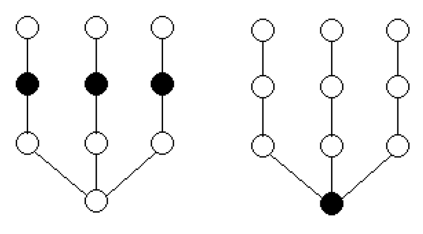
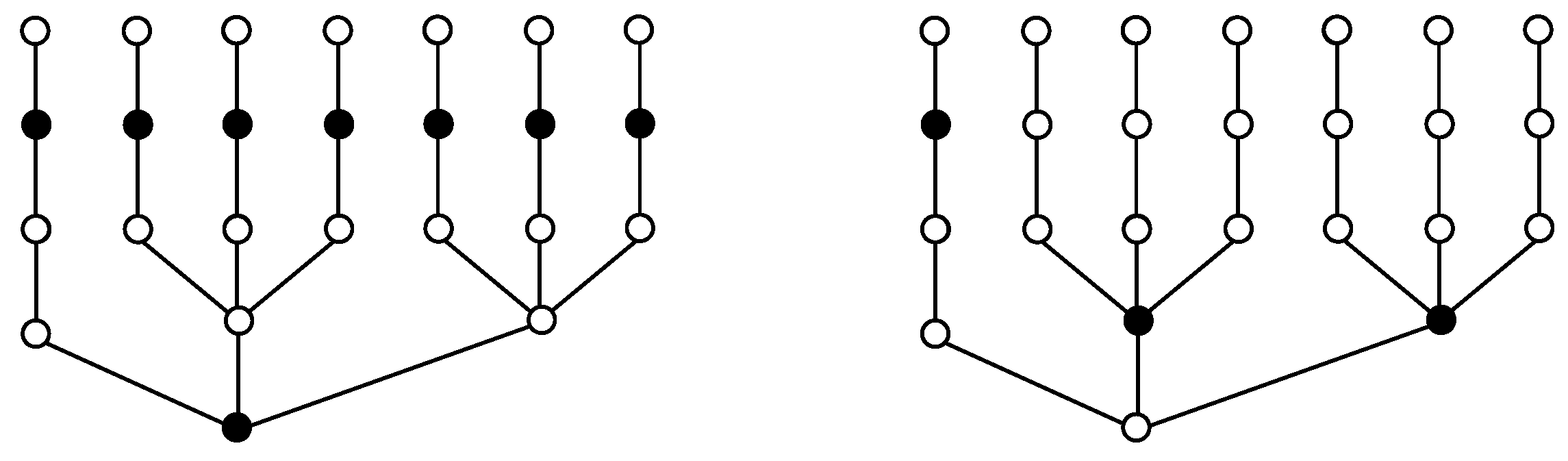
Note that the trees shown in Figure 1, Figure 2 and Figure 3, and the 1- and 2-differential sets marked (in black) suggest that if then . This question will be answered in Lemma 3.
Lemma 3.
Let be a graph. If , and there is no such that and , then for every such that and , we have .
Proof 7.
Let and be such that and . By hypothesis , so . Hence
Therefore, if , then , a contradiction. ☐
Lemma 4.
Let be a graph. If , then for every -differential set and every -differential set it is satisfied and .
Proof 8.
By absurdum we suppose that . Since , then
Therefore,
Since , we have a contradiction.
Finally, since , we have
☐
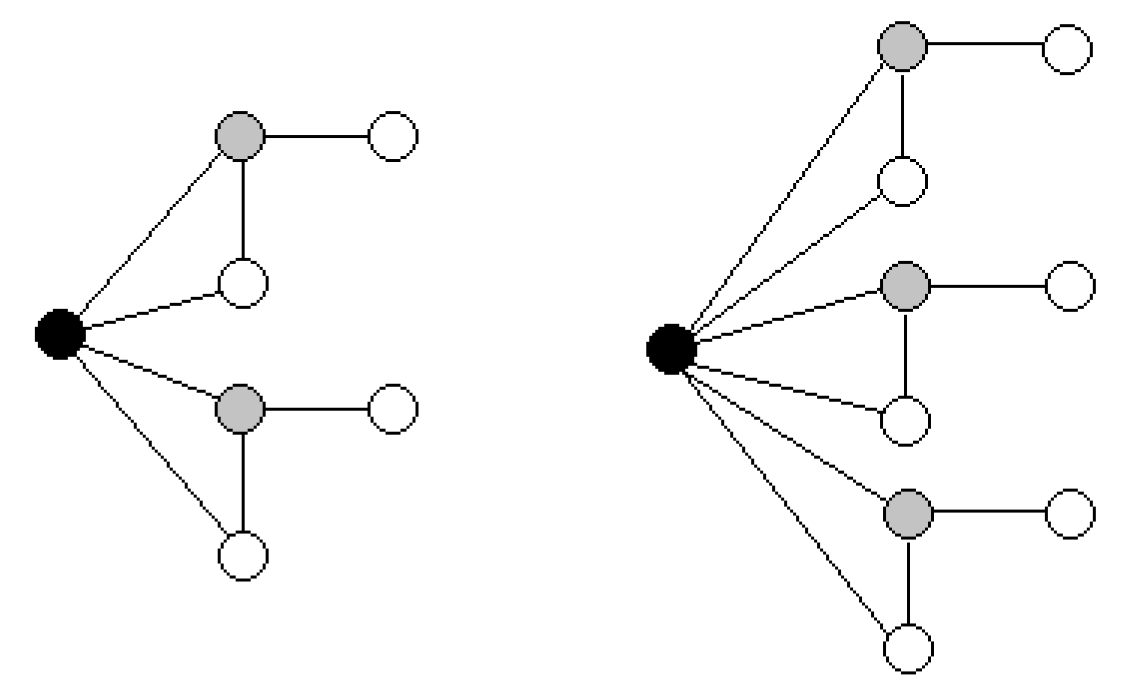
Looking also Figure 1, Figure 2 and Figure 3, it might be thought that every minimum -differential set is included in a maximum -differential set, but this is not true, as we can see in Figure 4, where black vertices sets are the minimum 1-differential set and -differential set, respectively, and grey vertices set are the maximum 1-differential set and -differential set, respectively.
If is an irrational number, then , because implies that .
Proposition 5.
Let be a graph. If and there exists such that and , then for every it holds and .
Proof 9.
Let and let be a -differential set, by Lemma 4 we have
thus, . Finally, since D is a -differential set, by Lemma 4, we have . Using now that D is also a -differential set, we have . The equality can be obtained analogously. ☐
Theorem 1.
Let be a graph, then the function is continuous for every .
Proof 10.
It follows from Lemma 3 and Proposition 5 that the graphic representation of the function is formed by pieces of straight lines with negative slope. That is, there exists a partition of such that
where . Moreover, and . Observe that is a continuous function because, if , then there exist and such that , so , since it is a maximum, should be equal to , a contradiction. ☐
For instance, in the graphs shown in Figure 5 we have if and if .
Notice that from the point of view explained in the introduction, if the cost of building a supermarket is (that is ), it is more profitable to build three supermarket giving service to all the towns. However, if the cost of building a supermarkets is (that is ), it is more profitable to build only one supermarket, leaving without service to three towns.
Note that there exist another generalizations in graphs using continuous parameters, for instance, -domination number in [19], where the resulting function is not continuous.
It might be also thought that the intervals where the function is a straight line are big, but there are graphs where these intervals are really small. For instance, if we consider the graph with vertices shown in Figure 6, the -differential set is an unitary set containing the black vertex when , and the set containing the grey vertices when .
As for every -differential set in , we can consider a graph G whose vertices are and edges . In such a case, the partition of the interval for the definition of the piecewise function is .
3. Bounds on the -Differential of a Graph
As we have mentioned in the introduction, will be the maximum benefit we could obtain if the cost of placing the considered service is , so it will be interesting to get lower and upper bounds for this benefit.
Proposition 6.
Let be a graph with order n and maximum degree Δ. Then
Proof 11.
Let such that . Then . Now, for any -differential set D we have that
☐
Proposition 7.
Let be a graph with order n and maximum degree Δ. The following properties hold.
- (a)
- if and only if .
- (b)
- if and only if .
- (c)
- If , then if and only if .
Proof 12.
- (a)
- If , by Proposition 6 we have , then . If and D is a -differential set, then we have . Therefore, , that is, and , which means that .
- (b)
- If , by Proposition 6 and (a) we have . If D is a -differential set such that , then , consequently, . Since , we have , which is a contradiction. If D is a -differential set such that , by and (a) we obtain , so . Now, if , there exists a -differential set D such that , therefore . By (a) we know that , then and, using again that , we conclude that , which means that .
- (c)
- If , there exists a -differential set D such that , then . By (a) we know that . If , then we have and , which is a contradiction with the fact that . Therefore, and, consequently, , which means that . Finally, if and D is a -differential set, by Proposition 6 we have , then or . If , since , we have and , a contradiction. If , since , we have and .
☐
Let us note that, if we consider the path with five vertices and , then we have but .
To characterize the graphs G such that is much more difficult. A characterization of these graphs when was given in [5], but only for trees. Next we will give some properties that the graphs verifying that equality must satisfy.
Proposition 8.
Let be a graph with maximum degree Δ. If and is such that , then:
- (a)
- .
- (b)
- for every .
- (c)
- for every .
Proof 13.
We suppose that and we take any vertex such that . If , there exist such that for every and . In such a case, , a contradiction. If there exists such that , then , a contradiction. If there exists such that , then , a contradiction. ☐
Note that conditions (a)–(c) in the above Proposition are not enough to guarantee that . The graph G shows in Figure 7 satisfies these three conditions but .
Proposition 9.
Let be a graph with order n and maximum degree Δ. If and , then . Moreover, if , then .
Proof 14.
The first statement is directly obtained by Proposition 8. Assume that and . If , then , a contradiction. ☐
Another lower and upper bound is shown in the following lemma.
Lemma 5.
Let be a graph with order n. Then
Proof 15.
For any set of vertices D it is known that . Therefore, for any -differential set D we have
Finally, if D is a minimum dominating set, then . ☐
Next, we will characterize all trees attaining the upper bound given in this lemma. For that, we will need the following result. We recall that a wounded spider is a graph that results by subdividing at most edges of the complete bipartite graph .
Lemma 6
([20]. If is a tree, then if only if G is a wounded spider.
Theorem 2.
If G is a tree of order n, then if only if G is a wounded spider.
Proof 16.
Assume that , and let D be a -differential set of G. Since and we know that , we deduce that for some , and . Therefore, and, by Lemma 6 we have that G is a wounded spider. If G is a wounded spider, again by Lemma 6 we have that , so . Finally, using Lemma 5 we conclude that . ☐
Proposition 10.
If is a graph with minimum degree δ. Then,
- (a)
- if , then ,
- (b)
- if , then .
Proof 17.
(a) Let S be a maximum open packing in G. If then , and so . The proof of (b) is analogous. ☐
Proposition 11.
Let be a graph with maximum degree Δ. If , then
Proof 18.
On one hand
On the other hand, if D is a -differential set, then and
☐
Proposition 12.
Let , and be the complete, path and cycle graph of order n and let and be the double star and the bipartite complete graph of orders and respectively. Then
If
Proof 19.
follows immediately from Proposition 6. Let with or . Let then Since any other set has -differential less than or equal to , then . Similarly, we can check the other cases. ☐
Lemma 7.
Let be a graph. If D is a minimum (respectively, maximum) β-differential set of G, then (respectively, ).
Proof 20.
If D is a minimum -differential set, then for every , the number k of vertices in which are adjacent to v but not to any , that means that they are private neighbors of v with respect to D, must satisfy , and so . If we consider the same situation when D is a maximum -differential set, it must be satisfied , that is, . ☐
Observe that when .
Proposition 13.
Let be a graph. If D is a β-differential set of G, then . Moreover, if D is a minimum β-differential set, then .
Proof 21.
It is enough to prove the first statement for a maximum -differential set. By Lemma 7 we have , so . If D is a minimum -differential set, Again by Lemma 7 we have , so ☐
Theorem 3.
Let be a graph with maximum degree Δ.
- (i)
- If , then
- (ii)
- If , then
Proof 22.
(i) Let D be a 1-differential set of G. Since , we have
(ii) Let D be a 1-differential set of G. Since , by Proposition 13 we have
then or, equivalently . ☐
Theorem 4.
Let be a graph of order n and minimum degree δ, and let . Then,
Proof 23.
Let D be a minimum -differential set. Since we have that every vertex in has at least one neighbor in , that is, is a dominating set. On one hand, since , we have . Now, using that, by Proposition 13, , we have
☐
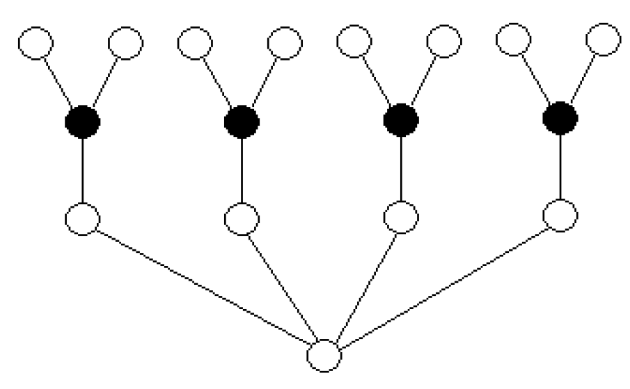
Note that (i) in Theorem 3 is attained for any graph with order n and maximum degree . On the other hand, (ii) is attained in any double star, like the one shown in Figure 8, when and .
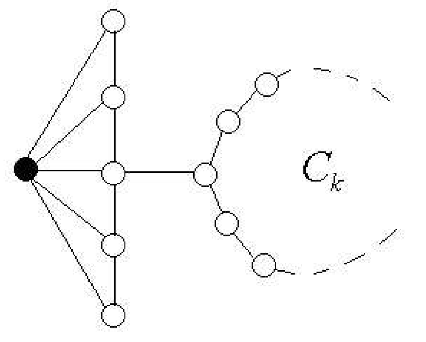
On the other hand, notice that, if it is not possible to give a bound similar to the one given in Theorem 4. For instance, it fails for the graph shown in Figure 9 with and , where represents a cycle of k vertices, we have and .
Theorem 5.
Let be a graph of order n, size m and maximum degree Δ. Then
Proof 24.
We note that if D is a minimum -differential set of G, then the following properties hold:
- (1)
- .
- (2)
- If , then .
- (3)
- If , then .
Let r be the number of edges from to . Then from (3) and (2) we have
Therefore,
In consequence, . ☐
We present now a technical lemma which will be used in the proof of Theorem 6.
Lemma 8.
If , then
Proof 25.
We write , where and , so the inequality is
or, equivalently,
Since is decreasing in and is increasing in , we have
☐
Theorem 6.
Let be a graph of order n, minimum degree δ and maximum degree Δ. Let and where . If , then
Proof 26.
We proceed by induction on k. For we suppose that and take such that . If there exists with , then for we obtain . Therefore, we can assume for every . Note that if there exists a such that , then
because . If we assume that for every , and hence . From Lemma 8 it follows
contradicting the hypothesis. Now, we suppose that the theorem is true for k and . Let be the collection of all -differential sets of G such that every satisfies that every vertex has at least external private neighbors with respect to D. That is, . Let with maximum cardinality. Since , by induction hypothesis we know that . Moreover, as , we also have .
If there exists such that , then we have
and we are done. Therefore, we suppose that for every it is satisfied . If is the number of edges in , then
We suppose that there exists and such that . If , then gives a -differential bigger than , which is impossible. If , then contradicting the choice of . Thus, we can assume that for any and , that is, for any and .
Let r be the number of edges between and . Then . Hence,
consequently,
or, equivalently,
Finally, using that , we obtain
and, as
we conclude that . ☐
Acknowledgments
We thank both referees for their valuable and constructive comments. This paper was supported in part by two grants from AEI and FEDER (MTM2016-78227-C2-1-P and MTM2015-69323-REDT), and a grant from CONACYT (FOMIX-CONACyT-UAGro 249818), Mexico. First author’s work was also partially supported by Plan Nacional I+D+I Grant MTM2015-70531 and Junta de Andalucía FQM-260.
Author Contributions
These authors contributed to equally to this work.
Conflicts of Interest
The authors declare no conflict of interest.
References
- Kempe, D.; Kleinberg, J.; Tardos, E. Maximizing the spread of influence through a social network. In Proceedings of the Ninth ACM SIGKDD International Conference on Knowledge Discovery and Data Mining, New York, NY, USA, 24–27 August 2003; pp. 137–146. [Google Scholar]
- Kempe, D.; Kleinberg, J.; Tardos, E. Influential nodes in a diffusion model for social networks. In Proceedings of the 32nd international conference on Automata, Languages and Programming, Lisbon, Portugal, 11–15 July 2005; pp. 1127–1138. [Google Scholar]
- Haynes, T.W.; Hedetniemi, S.; Slater, P.J. Domination in Graphs: Advanced Topics; Taylor and Francis: Didcot, UK, 1998. [Google Scholar]
- Bermudo, S.; Fernau, H. Lower bound on the differential of a graph. Discret. Math. 2012, 312, 3236–3250. [Google Scholar] [CrossRef]
- Mashburn, J.L.; Haynes, T.W.; Hedetniemi, S.M.; Hedetniemi, S.T.; Slater, P.J. Differentials in graphs. Util. Math. 2006, 69, 43–54. [Google Scholar]
- Basilio, L.A.; Bermudo, S.; Sigarreta, J.M. Bounds on the differential of a graph. Util. Math. 2015, in press. [Google Scholar]
- Bermudo, S. On the Differential and Roman domination number of a graph with minimum degree two. Discret. Appl. Math. [CrossRef]
- Bermudo, S.; De la Torre, L.; Martín-Caraballo, A.M.; Sigarreta, J.M. The differential of the strong product graphs. Int. J. Comput. Math. 2015, 92, 1124–1134. [Google Scholar] [CrossRef]
- Bermudo, S.; Fernau, H. Computing the differential of a graph: Hardness, approximability and exact algorithms. Discret. Appl. Math. 2014, 165, 69–82. [Google Scholar] [CrossRef]
- Bermudo, S.; Fernau, H. Combinatorics for smaller kernels: The differential of a graph. Theor. Comput. Sci. 2015, 562, 330–345. [Google Scholar] [CrossRef]
- Bermudo, S.; Fernau, H.; Sigarreta, J.M. The differential and the Roman domination number of a graph. Appl. Anal. Discret. Math. 2014, 8, 155–171. [Google Scholar] [CrossRef]
- Bermudo, S.; Rodríguez, J.M.; Sigarreta, J.M. On the differential in graphs. Util. Math. 2015, 97, 257–270. [Google Scholar]
- Pushpam, P.R.L.; Yokesh, D. Differential in certain classes of graphs. Tamkang J. Math. 2010, 41, 129–138. [Google Scholar] [CrossRef]
- Sigarreta, J.M. Differential in cartesian product graphs. Ars Comb. 2016, 126, 259–267. [Google Scholar]
- Hernández-Gómez, J.C. Differential and operations on graphs. Int. J. Math. Anal. 2015, 9, 341–349. [Google Scholar] [CrossRef]
- Goddard, W.; Henning, M.A. Generalised domination and independence in graphs. Congr. Numer. 1997, 123, 161–171. [Google Scholar]
- Zhang, C.Q. Finding critical independent sets and critical vertex subsets are polynomial problems. SIAM J. Discret. Math. 1990, 3, 431–438. [Google Scholar] [CrossRef]
- Slater, P.J. Enclaveless sets and MK-systems. J. Res. Nat. Bur. Stand. 1977, 82, 197–202. [Google Scholar] [CrossRef]
- Dahme, F.; Rautenbach, D.; Volkmann, L. Some remarks on α-domination. Discuss. Math. Gr. Theory 2004, 24, 423–430. [Google Scholar] [CrossRef]
- Domke, G.S.; Dumbar, J.E.; Markus, L.R. Gallai-type theorems and domination parameters. Discret. Math. 1997, 167–168, 237–248. [Google Scholar] [CrossRef]
Figure 1.
and .

Figure 2.
.
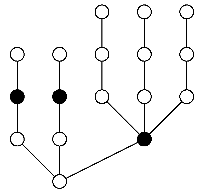
Figure 3.
and .

Figure 4.
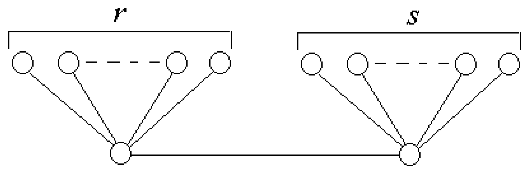
On the left and , and on the right and .

Figure 5.
-differential set when (on the left) and -differential set when (on the right).
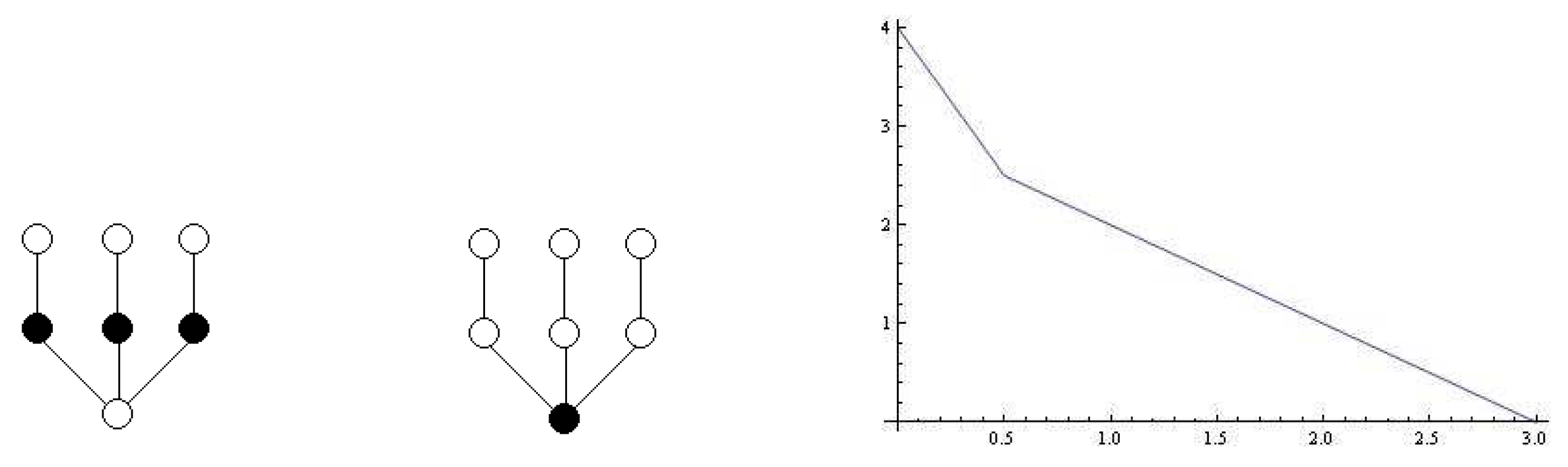
Figure 6.
An example of a graph such that if , and if .

Figure 7.
An example with and .

Figure 8.
This graph show that the bound (ii) in Theorem 3 is attained when and .

Figure 9.
This graph show that Theorem 4 can fail when .

© 2017 by the authors. Licensee MDPI, Basel, Switzerland. This article is an open access article distributed under the terms and conditions of the Creative Commons Attribution (CC BY) license (http://creativecommons.org/licenses/by/4.0/).
Share and Cite
MDPI and ACS Style
Basilio, L.A.; Bermudo, S.; Leaños, J.; Sigarreta, J.M. β-Differential of a Graph. Symmetry 2017, 9, 205. https://doi.org/10.3390/sym9100205
AMA Style
Basilio LA, Bermudo S, Leaños J, Sigarreta JM. β-Differential of a Graph. Symmetry. 2017; 9(10):205. https://doi.org/10.3390/sym9100205
Chicago/Turabian StyleBasilio, Ludwin A., Sergio Bermudo, Jesús Leaños, and José M. Sigarreta. 2017. "β-Differential of a Graph" Symmetry 9, no. 10: 205. https://doi.org/10.3390/sym9100205
Note that from the first issue of 2016, this journal uses article numbers instead of page numbers. See further details here.