Polar Bear Optimization Algorithm: Meta-Heuristic with Fast Population Movement and Dynamic Birth and Death Mechanism


Institute of Mathematics, Silesian University of Technology, Kaszubska 23, 44-100 Gliwice, Poland
*
Author to whom correspondence should be addressed.
Symmetry 2017, 9(10), 203; https://doi.org/10.3390/sym9100203
Submission received: 7 September 2017
/
Revised: 21 September 2017
/
Accepted: 25 September 2017
/
Published: 28 September 2017
(This article belongs to the Special Issue Information Technology and Its Applications)
Abstract
:In the proposed article, we present a nature-inspired optimization algorithm, which we called Polar Bear Optimization Algorithm (PBO). The inspiration to develop the algorithm comes from the way polar bears hunt to survive in harsh arctic conditions. These carnivorous mammals are active all year round. Frosty climate, unfavorable to other animals, has made polar bears adapt to the specific mode of exploration and hunting in large areas, not only over ice but also water. The proposed novel mathematical model of the way polar bears move in the search for food and hunt can be a valuable method of optimization for various theoretical and practical problems. Optimization is very similar to nature, similarly to search for optimal solutions for mathematical models animals search for optimal conditions to develop in their natural environments. In this method. we have used a model of polar bear behaviors as a search engine for optimal solutions. Proposed simulated adaptation to harsh winter conditions is an advantage for local and global search, while birth and death mechanism controls the population. Proposed PBO was evaluated and compared to other meta-heuristic algorithms using sample test functions and some classical engineering problems. Experimental research results were compared to other algorithms and analyzed using various parameters. The analysis allowed us to identify the leading advantages which are rapid recognition of the area by the relevant population and efficient birth and death mechanism to improve global and local search within the solution space.
MSC Classification:
80M50; 90C59; 70H451. Introduction
Increasing technological development makes the accuracy becoming the most desirable element in applied modeling. It is essential, so that the cost of the product or the amount of work will be as small as possible. Moreover exactly calculated dimensions, volume, or any other parameter can make our lives and our work more effective, simpler and enjoyable. The problem of accuracy comes to finding optimal solutions for given problems from engineering, architecture, medicine, etc. Through these areas, a heuristic approach to solving problems turned out to be a successful tool. It becomes more and more popular due to numerous features, such as speed of finding optimal solutions and low computational complexity.
One of very good examples for heuristic implementations is environmental engineering. Increasing pressure to reduce pollutants produced during production of heat, car engines, etc. motivates scientists to seek alternative methods of treatment. An alternative to existing fuel industry is biofuel that is biomass produced by living organisms. The use of heuristics in this topic makes it possible to estimate potential outcome of the region for possible variety of liquid biofuels as shown by [1]. Diesel engines operating on oil, even when using a particulate filter, produce large quantities of harmful vapors. Application of heuristics in diagnosis and analysis of these engines is shown by [2]. Interesting aspect of energy production was presented by [3]. In the research, optimization of components for PV-wind-diesel-battery was done by the use of stochastic and meta–heuristic methods. Problems with pollution and numerous threats of earthquakes cause the location of homes on affected areas to be of a paramount importance. [4] presented positioning of networking systems by nature based optimization methodology. [5] presented that a model of a real-time seismic monitoring and early warning system for earthquakes can be based on devoted heuristic optimizer. [6] presented that heuristic algorithms can be applied in the design of steel structured houses that have been built in areas affected by seismic movements.
Related Works
Methods for solving optimization problems like heuristics do not guarantee obtaining the result identical with analytical solution. Depending on the initial population, we might expect faster or slower convergence to analytical solutions. However as the research show these methods give very precise results. Therefore it is important to constantly work on new efficient algorithms. Heuristics simulate phenomena that occur in nature into optimization algorithms. Different approaches make use of various selective strategies implemented into optimization algorithms. There are many propositions to simulate the way animals hunt and breed. Selecting a right place to settle is also a very important strategy, in which an animal adapts to environmental conditions to achieve the best possible result. Hunting is inevitably linked to the prey and local environment. Different conditions involve a lonely hunting behavior or hunting in a herd. In the first, an animal uses various aspects of smell, hearing, sight which are altogether combined into efficient actions for optimal hunting strategy. On the other hand, while hunting in a group the animals depend on other members of the herd, which all cooperate to corner the prey. Similarly other phenomena from the nature can inspire optimization methods. Water running on the surface of the ocean is adapting to weather conditions in which a cylindrical shape gives to the waves optimal strength of action. These are very similar to optimization, where the algorithm must adapt to given criterion for the best possible solution. We can find many models based on animals strategies and nature phenomena composed into optimization strategies.
Simulated Annealing (SA) is one of the first proposed meta-heuristics [7]. In this method annealing process is simulated in the search space to find the optimum for modeled functions. In [8] was presented an idea of Genetic Algorithm (GA), which is simulating processes of genetic evolution into optimization purposes. Particle Swarm Optimization (PSO) was presented in [9]. This method is based on a model of the swarm of individuals that cooperate together to optimize the strategy for development. Another interesting example of the swarm intelligence is Artificial Bee Colony Algorithm (ABCA) presented in [10]. This method simulates the behavior of ants while traversing the habitat in search for food. One of heuristics based on stochastic theory is Cuckoo Search Optimization Algorithm (CSA) described by [11]. Proposed model simulates behavior of cuckoos while tossing their eggs into nests of other birds. The movement of individuals in the search for the optimal location is described using Lévy flight approach. The phenomenon of echolocation used by bats have been modeled in Bat Algorithm (BA) by [12]. This algorithm simulates hunting bats, which are using natural radar to trace the prey. Firefly Algorithm (FA) was introduced in [13], where the author presented an idea to model relations between individuals in a swarm of fireflies. In that heuristic a model of communication between bugs searching for an optimal partner is implemented into optimization algorithm. Not only behavior of animals has been subjected to mathematical analysis, but also phenomenon of plants growth. Flowers Pollination Algorithm (FPA) presented by [14] brings a model of flower pollen raised by the wind. Recent years brought other models sourced in nature phenomena. In [15] was shown a model of breaking sea waves called Water Wave Optimization Algorithm (WWO). The particles of the wave inspired optimization strategy, which simulates the cylindrical movements of the water on the surface of the ocean. In [16] was proposed the model of moths movements to the light based on spiral trajectory formulated in Moth-Flame Optimization Algorithm (MFO). Predation of dragonflies was formulated in Dragon-Fly Algorithm (DA) in [17].
These algorithms have presented a dedicated modeling of various aspects taken from the nature of living species and weather phenomena. Some of the strategies present a swarm communication models, the other use single individual actions to simulate optimization. Among them we have models of organisms on various levels of evolution and also various families of fauna and flora. We have models of birds, models of bugs, models of cell evolutions but at the same time we have models of flowers and water waves. Some of these methods have clearly visible two stages of modeling: global and local search. Depending on the proposed model the algorithms can have fast convergence to the optimum. However still important aspect is the location of the initial population. The starting points may influence the final results. Therefore the best option to compose a meta-heuristic algorithm is to define a composition of efficient approaches that will support the highest performance for each of the optimization stages. The algorithm shall be efficient in the global search, since this phase makes it possible to search the entire model space. A precision of the results depends on the local search, in which the algorithm is correcting the final values in the local sub domain. Each of the methods must be possibly low complex for fast computations. Therefore one of the possible aspects is to efficiently control the number of individuals in the population.
In this article, we propose to model behavior of polar bears while searching for food over frosty arctic land and sea into optimization strategy, see Figure 1. Polar bears have a very difficult environment for their development, yet these animals achieved optimal results becoming rulers of the arctic. This gave us an inspiration for the research on possible modeling of their behavior into heuristic algorithm. In the model we assume that the domain for the optimization is very similar to arctic conditions. We do not know where the optimums are. Similarly polar bears do not know where to find seals or other food. In the search we can be trapped in local optima, what can prevent us from global optimization. Moreover the nature of optimized objects and functions can be difficult and so the optimization needs some specific strategies to avoid mistakes. Polar bears search for food but the arctic conditions can make them trapped and even die, so they developed very efficient mechanisms that help them to succeed. We have distinguished two phases of the hunting strategy. One we simulate for a global search, the other for a local search. A model of searching for food through the arctic lands and waters gave a very promising global search. We adopted travel through the arctic for a search of sub domains with possible optimum. While in each iteration of the algorithm local search is simulated using model of specific hunting. Additionally the proposed model introduces a mechanism to control birth and death processes, which stimulates the number of individuals similarly to the nature conditions.
The novelty of the proposed method is in the efficient composition of these three nature-inspired mechanisms into one heuristic algorithm. Each of them represents some important aspect of the adaptation of polar bears to the arctic conditions that help them to succeed. Proposed model makes use of these actions implemented into optimization strategy, in which we can efficiently search through the entire domain. The model prevents blocking in the sub spaces of the local minima. While proposed birth and death strategy enables dynamic adaptation to the optimized model, without using large population of individuals in each iteration.
2. Polar Bear Optimization Algorithm (PBO)
Polar bears are mammals inhabiting icy territories of the Arctic, where they are the biggest predators (see [18]). This privilege is caused by their adaptation to the environment and the special hunting behaviors. Their external adaptation to the environment plays a minor role, although very useful. A thick layer of fat prevents polar bears from cooling their organisms and white fur enables a camouflaged appearance amongst the ice and snow. The other factors play a major role in survival of polar bears in harsh arctic climate. Behavioral factors made polar bears able to hunt and survive.
The advantage comes with the speed of attack and the way of movement, even on long distances over cold waters. Polar bear jumps on ice floe and drifts on it to places where better feeding occasions may occur. Proposed model of displacement of the polar bear on an ice floe is illustrated in Figure 2. After reaching destination hunting is done by surrounding the victim in search for the best position to attack. This behavior can be modeled using proposed trifolium equation. Figure 3 shows the movement of the polar bear before the attack. Although polar bears prefer to consume seals, they also eat fish and other animals that come within their reach. During one meal adult polar bear eats nearly 60 kg of raw flesh, so he needs to hunt often. We propose mathematical model of these behaviors to be used as optimization strategy.
2.1. Basic Premise
In the proposed algorithm we assume that population of hunting polar bears is composed of a certain number of k individuals. Each individual (polar bear) is represented as a point of multiple n coordinates described as . In order to distinguish each polar bear in a whole population in a given iteration t, we introduce the following definition of the individual: , where i is the number of polar bear and j is given coordinate. The natural habitat of these mammals (the Arctic) will be interpreted as a solution space for a given optimization problem. The population of polar bears will move over the solution space to find the optimum values according to the initial criteria.
Definition of the Optimization Problem
Let be the function of n variables, and i-th point in the solution space for will be defined as . Then if the value of the function is global minimum or maximum on , then is the optimal solution.
2.2. Global Move Using Ice Floes
If a hungry polar bear does not find anything to eat in his nearest area then he enters a large and stable ice floe which does not break under his weight for a long period. He uses it to drift toward remote locations with possible habitats of seals. Drifting may take several days during which he looks for food in the surrounding lands and waters.
The displacement of the individual over a large distance with the constant analysis while passing through the area is hard to implement due to the large number of possible calculations. For this reason, the phenomenon of the movement on the ice floe was interpreted as the movement of the polar bear toward one of the fittest individuals (*) in the whole population in t-th iteration as
where is a random number in interval , is the distance between two spatial coordinates and is a random value in the range of . The distance is understood as Euclidean metric between points and , and it is defined as
The presented motion model represents global search and it is performed for each individual in the iteration, however positions are changed only in case of finding better locations. We modeled the global movement toward the fittest individual since we assume that all the bears are hunting. Therefore if any of them is closer to the possible habitat of seals his position appears to be promising for further search for the optimum. Illustration of this process is shown in Figure 2.
2.3. Local Search While Hunting Seals
During hunting polar bears slowly roam arctic lands in order to detect potential prey. Not only the land surface is observed, but also sea waters. In case of spotting prey, the bear quietly moves closer to find the optimal position. When he approaches close enough to attack or he is noticed by the animal, he moves as fast as he can to catch the prey. Seals most often like to stay on the ice, however they jump into the water when they feel any danger. The hunting polar bear without hesitation jumps after the seal into the water. Swimming and diving are additional advantages of polar bears, which allow them to become one of the largest predators in arctic areas. Polar bear moves very quickly under the water and reach the victim by stabbing teeth into the body of a seal then pulls it out of the water onto the floe surface where he eats it.
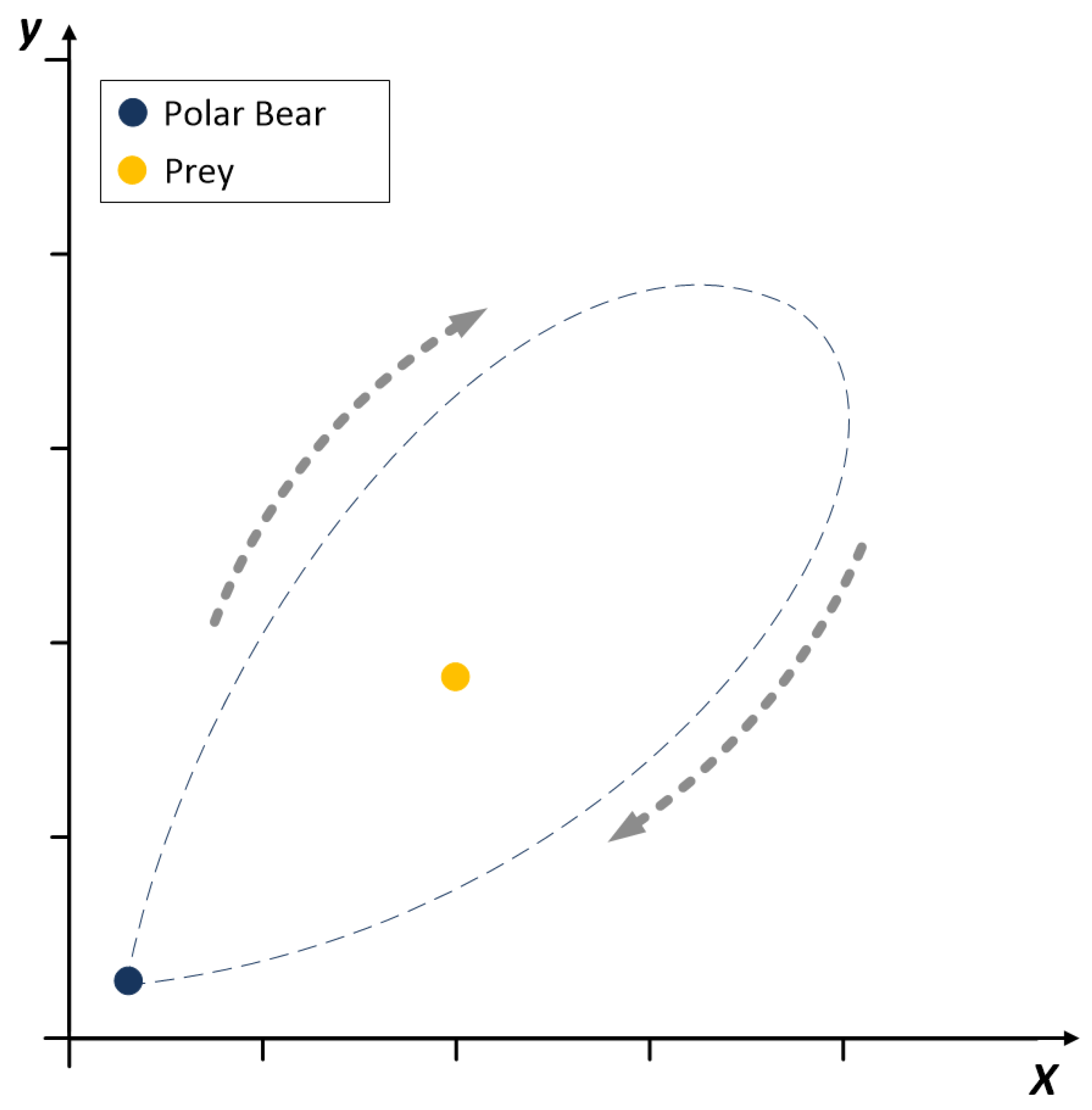
We have modeled a specific movement while hunting seals as the local search. Movement of each individual was visualized as a movement along modified excerpt from the trifolium equation starting from the current position of the polar bear. The radius of the view of a polar bear can be represented by two parameters: which regulates the distance in which polar bear can see the seal, and the angle of the tumbling around the victim. These parameters are used to define vision radius as
The radius is used in description of movements of individuals in the population by the following system of equations for each spatial coordinate
where each of the angular values is selected at random for each point in accordance with . In the course of looking around for food, polar bear verifies position in the front (then mark ± is replaced by +). If the new position is worse than current, the bear looks around on the other side (in this situation ± is replaced by −). Equation (4) simplified to simulate the movement on two–dimensional plane is reduced to motion along modified equation of the single trifolium’s leaf. Sample of this movement is shown in Figure 3. Polar bear starts to move and staggers back looking for food to take better position to attack. In PBO algorithm, this situation is illustrated by selecting a random position on the leaf which corresponds to the local search optimization phase.
2.4. Dynamic Population Control by the Reproduction and Extinction by Starvation
At the beginning of the algorithm the population of polar bears consists only of of created individuals. The remaining depends on population growth and represent reproduction of the best individuals or starvation of the worst.
In each iteration of the algorithm, individual can die due to the arctic conditions or reproduce after successful hunting. This operation represents the influence of the arctic weather and harsh environment, which in the PBO algorithm introduce necessary randomness to the optimization strategy. We introduce chosen at random in each iteration. Depending on this value, the operation is performed in accordance with
The death of the weakest individuals in the population is performed under condition that the population size will not be lower than of the given number. Reproduction of two individuals and (from the top rated among all in t-th iteration except the best one) into a new individual is
These operations give the dynamic control over the population of polar bears. The maximum and the minimum numbers of individuals are not exceeded since the reproduction and extinction are performed only to keep the number of bears in the population at the same level. In this way, we model the polar bear behaviors due to his way of hunting in arctic environment. Complete algorithm is shown in Algorithm 1.
| Algorithm 1: Polar Bear Optimization Algorithm |
|
3. Experimental Results for Classic Test Functions
In the benchmark tests to evaluate performance of the PBO algorithm we have used 13 sample functions presented in Table 1. These test functions are often called artificial landscapes. Some of these functions are smooth surfaces for which there is no local minimum that can make the algorithm stuck. Smooth functions are mainly spherical shapes (Nos. 6, 9 and 10), flat (No. 13), or valley shaped (Nos. 1 and 5). The other are rough landscapes representing mountain terrain, e.g., areas with many local minima and only one global minimum (see functions Nos. , , ).
These functions were used in benchmark tests to compare found optimal solutions by proposed method and 11 other meta-heuristic algorithms. All results were compared regard to the accuracy and the average speed of finding solutions. In addition, proposed PBO was examined for the efficiency of the proposed dynamic population control. We have calculated the change in the number of individuals in the population, the average adaptation of the whole population and convergence during following iterations. The results are presented in Figure 4. Each test function was optimized 100 times by each of the algorithms: BA ([12]), CSA ([11]), DA [17]), FA ([13]), FPA [14]), MFO ([16]), WWO ([15]), SA ([7]), GA ([8]), PSO ([9]), AACA ([10]) and proposed in this article PBO.
In each benchmark test the same parameters have been set: population composed of 100 individuals and 100 iterations. Average values of the best individuals from 100 runs are shown in Table 2. Comparison of presented experimental results show that PBO is a good alternative to other meta-heuristics. Resulted optimal solutions for most of test functions are very precise. The results of PBO turned out to be the most accurate next to MFO and PSO algorithms. MFO proved to be more accurate primarily for Schwefel’s function which has many local minima, while PBO for Sphere function. In Table 3 are presented standard deviations of optimization results. PBO values for functions Nos. 2, 6, 9, 11 and 12 are very low. If compared to other methods, PBO values are the lowest in many cases. Standard deviations are always less than what means that obtained solutions are not significantly scattered. Wilcoxon rank-sum test was performed for all the solutions and resulted p-values are shown in Table 4. Only two methods gave p-value higher that . These were FPA and PBO for Shubert’s function, what shows that statistically these are the best methods.
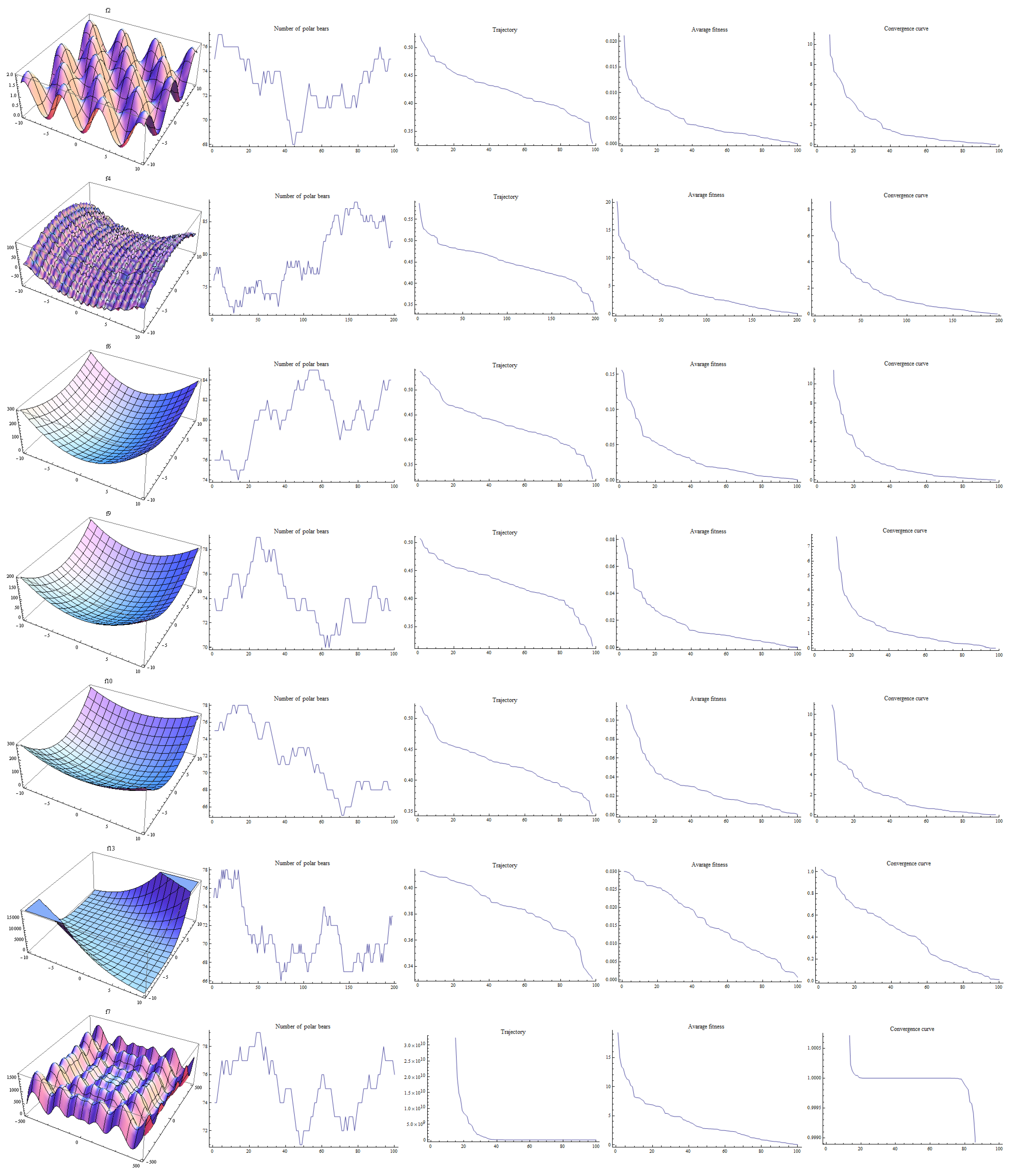
In Figure 4 were plotted measurements of various parameters for selected test functions:
- average number of individuals in the population according to their fertility and mortality,
- average trajectory with respect to the ideal solution,
- average adaptation of the population,
- rate of convergence.
The initial state of the population was set to 75 individuals with an upper limit of 100 individuals. During 100 iterations, the average number of individuals never reached at maximum. Only in rare cases, PBO achieved a number higher than for functions Nos. 4 and 5 (Rastragin and Rosenbrock). Modeled technique of dynamic birth and death control of polar bears indicates reduction in the number of calculations by removing the worst individual. Moreover it enables to gain better solution by combining two among the best individuals. For all meta-heuristics, to have more accurate optimization results it is necessary to increase the number of individuals or iterations. For proposed PBO this can also help what can be seen in a chart showing change in positions of points according to the Euclidean metric described by Equation (2). We see small and medium value changes from iteration to iteration. Fastest changes take place on the interval 80–100 iterations for each test function. The most interesting case for this analysis is Schwefel’s function. The changes are minimal, and above 40 iterations they are almost unnoticeable. The reason for this situation are landscape features. Many local minima do not allow to exit points, what results in no change in the trajectory. Medium changes in adaptation to applied test functions are heading to exact solution with each iteration. It can be seen in examples, where the curve is heading quickly to 0. It is similar with ratio of convergence, where the curves are heading quickly to the exact solution. Only for Schwefel’s function, the rate of convergence stuck between 20 and 80 iterations what may be caused by decreasing amount of polar bears in this period. Along with increased number of bears, rapid minimization of this rate occurred. For most functions proposed control procedure has proven to be an effective solution. Schwefel’s function has contributed to a large number of stops in the algorithm. The reason may be not perfect choice of parameters, especially the number of subjects or distance vision of individuals with such a large number of local minima.
4. Application of PBO in Engineering Problems
Engineering problems involve positioning systems to balance operation characteristics of selected elements to work at minimal cost in certain purposes. In this section we would like to present classic problems solved by applied heuristics in order to show efficiency of the proposed method in engineering applications. Each of analyzed problems has been subjected to comparative analysis.
4.1. Pressure Vessel Design Problem
Compressed air tank is a gas storage container (for instance liquid air) that under a certain pressure keeps the content using pressure compressor or accumulator to control interior atmosphere. The problem lies in the design of a tank with the maximum pressure of 1000 [psi] and the minimum volume of 750 [ft]. Let’s assume that it will be a specific type of a tank called cylindrical pressure vessel (presented in Figure 5) with hemispherical cylinders at both ends.
Physically, the vector of the entire construction can be represented by four variables
- —the coating thickness of cylinder,
- —the coating thickness of hemispherical cylinders,
- —the radius of the cylinder without it’s shell,
- —the length of the cylinder.
The designing problem is to minimize the cost of production. Minimizing production cost means minimizing the weight of the tank what may be represented by the following function
where and . In addition, the following conditions – should be taken into consideration
Similarly to the results of benchmark test functions optimization presented in Section 3, other meta-heuristic methods were compared to the proposed BPO. All algorithms were executed with 100 individuals in the population and 100 iterations. Each test was performed 100 times, the average values are presented in Table 5. The results show that proposed PBO method along with MFO and PSO are the most accurate for this problem.
4.2. Gear Train Problem
The gear train includes four round gear wheels with straight teeth. The problem is to minimize the gear ratio specified as follows
where represent following gears in accordance with the scheme in Figure 6.
Averaged results of minimal gear ratio are shown in Table 6. PBO algorithm proved to be the best solution for obtaining better solution from the MFO algorithm.
4.3. Welded Beam Design Problem
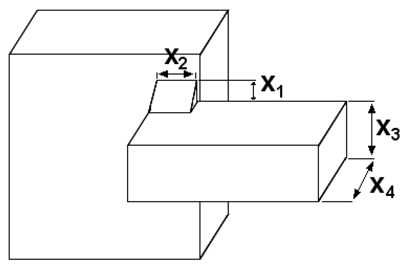
Welded beam is composed of two components – beam and weld. The problem of construction design is to minimize the cost of the weld and material of the beam with condition of deflection of the beam. The design model illustrated in Figure 7 can be described by the following equation
where and and mean physical quantities like height of x, length of x, height of the beam and width of the beam, respectively. In addition, the following conditions – should be taken into account
which are modeled using following equations
The following values were selected as parameters to analyze the problem: [lb], [in.], [psi], [psi], [psi], [psi] and [in.]. Obtained results from different algorithms are presented in Table 7. PSO and MFO algorithms turned out to be the most accurate methods for this problem. Slightly worse result returned PBO algorithm, but it is still one of the best in comparison to other methods.
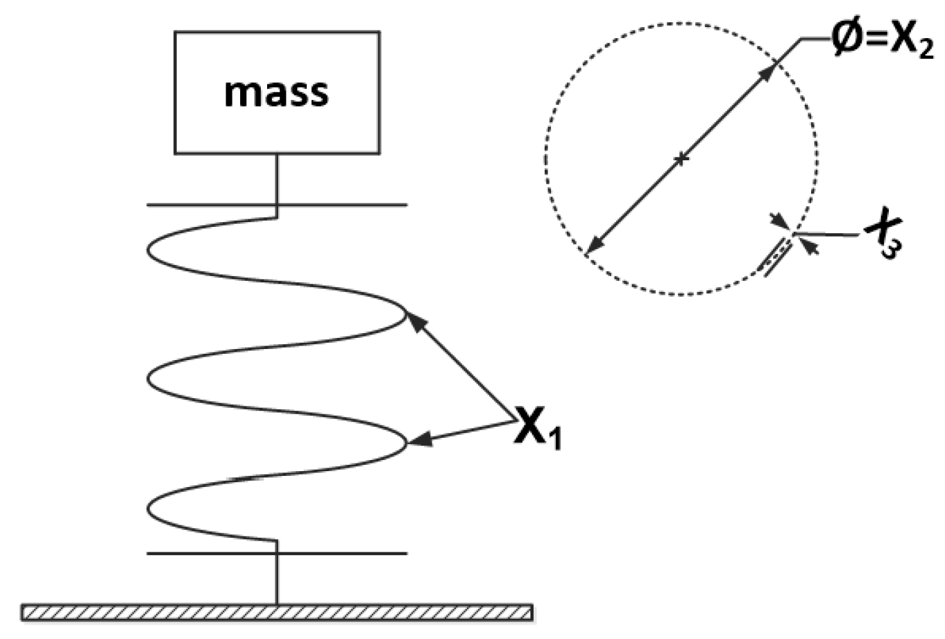
4.4. Compression Spring Design Problem
A spring is in action with a mounted load, where we have tension/compression reactions as presented in Figure 8. The problem of construction design is to minimize the spring volume during tension/compression reaction to the mounted load. The design model for active spring coils , winding diameter , and wire diameter can be described by the following equation
where we calculate the elements for the minimal volume of the spring by assumptions: , , , for which the stress constraints are
Obtained results from different algorithms are presented in Table 8. PSO with PBO were the best in this optimization problem, however all other tested heuristic algorithms achieved results very close to them.
5. Discussion
In the examinations we have verified the efficiency of the newly proposed heuristic method. Defined in this article, the Polar Bear Optimization Algorithm was tested using 13 classic test functions and examined as an optimization procedure for 4 designed problems: pressure vessel, gear train, welded beam and compression spring.
As a conclusion from the research we can say that proposed PBO is a valuable optimization method, which can be used to solve both theoretical and practical problems. The results for classic test functions have showed that PBO is reaching optimum values with good precision. The optimization process is smooth and the convergence to the optimum values is good. From the results for engineering problems we also conclude a good efficiency of the proposed PBO. Comparing to other examined heuristics the results of PBO were the best in some cases and in other experiments MFO and PSO received better results. Nevertheless proposed PBO was always one of the best algorithms.
The model of the BPO simulates two phases of the polar bears hunting defined as global and local searches. Additionally to these we have modeled efficient birth and death mechanism that is controlling the number of individuals in the population. Therefore using all these three in a one heuristic algorithm we have composed an efficient optimization algorithm. In the tests we have defined and as the most efficient level of coefficient used to control the population. Similarly the best results for the local search phase were achieved for . The coefficients used for model of the global search are selected at random therefore they do not influence the model and also enable better search in the whole domain. Since the control of the population makes the method use only the necessary number of individuals the computational complexity is lower. During iterations we perform only the necessary calculations. The number of individuals is not constant as for other heuristic methods but change in accordance to performance of the algorithm. In Figure 4 we can see how the number adopts to calculations during iterations of the algorithm. The PBO model is presented in a form usable for multidimensional search spaces. The coefficients used to compose the global search model are mostly selected at random, therefore PBO is able to search for optimums in various spaces where different constraints make the domain narrow.
For future research we think of some possible applications of devoted versions of this method. We think that potential application to some complex engineering problems will be possible due to the nature of the multidimensional composition of the algorithm. Probably some adjustments in the model coefficients will be necessary to exactly fit the model. In the research we have examined PBO in some classic engineering problems of low dimensions, the results were good and further developments of this method may benefit e.g. from fuzzification of some parts to flexibly fit all the optimized variables.
6. Final Remarks
In this article we proposed a novel heuristic paradigm that models the behavior of polar bears. The Polar Bear Optimization Algorithm models a global and local search with efficient model of motion and dynamic mechanism of births and deaths of individuals in the population. These aspects contributed to obtain competitive results in benchmark tests. Proposed dynamic mechanism reduces computational complexity by reducing the number of operations. The proposed algorithm has been tested not only for test functions but also for real design engineering problems. The experimental research showed that proposed algorithm proved to be one of the best in these calculations showing highest precision in optimization of modeled variables. Comparisons have shown high potential of the proposed algorithm for various applications but also for future development.
Acknowledgments
The authors would like to acknowledgment contribution to this research from the Rector of Silesian University of Technology under grant RGH 2017 No. 09/010/RGH17/0026 for prospective professors, which was received for covering the costs of this publication in open access. And also contribution from by the “Diamond Grant 2016” No. 0080/DIA/2016/45 funded by the Polish Ministry of Science and Higher Education.
Author Contributions
Dawid Połap and Marcin Woźniak designed the method, performed experiments and wrote the paper.
Conflicts of Interest
The authors declare no conflict of interest.
References
- Dusmanescu, D.; Andrei, J.; Popescu, G.H.; Nica, E.; Panait, M. Heuristic methodology for estimating the liquid biofuel potential of a region. Energies 2016, 9, 703. [Google Scholar] [CrossRef]
- Isermann, R. Fault diagnosis of diesel engines. Mech. Eng. 2013, 135, 64–74. [Google Scholar]
- Dufo-López, R.; Cristóbal-Monreal, I.R.; Yusta, J.M. Stochastic-heuristic methodology for the optimisation of components and control variables of PV-wind-diesel-battery stand-alone systems. Renew. Energy 2016, 99, 919–935. [Google Scholar] [CrossRef]
- Li, Y.H.; Wang, J.-Q.; Wang, X.J.; Zhao, Y.-L.; Lu, X.H.; Liu, D.L. Community detection based on differential evolution using social spider optimization. Symmetry 2017, 9, 183. [Google Scholar] [CrossRef]
- Lomax, A.; Satriano, C.; Vassallo, M. Automatic picker developments and optimization: FilterPicker—A robust, broadband picker for real-time seismic monitoring and earthquake early warning. Seismol. Res. Lett. 2012, 83, 531–540. [Google Scholar] [CrossRef]
- Kaveh, A.; Bakhshpoori, T.; Azimi, M. Seismic optimal design of 3D steel frames using cuckoo search algorithm. In The Structural Design of Tall and Special Buildings; John Wiley & Sons: Hoboken, NJ, USA, 2015; Volume 24, pp. 210–227. [Google Scholar]
- Van Laarhoven, P.J.; Aarts, E.H. Simulated annealing. In Simulated Annealing: Theory and Applications; Springer: Berlin, Germany, 1987; pp. 7–15. [Google Scholar]
- Holland, J.H. Genetic algorithms. Sci. Am. 1992, 267, 66–73. [Google Scholar] [CrossRef]
- Kennedy, J.; Eberhart, R. Particle swarm optimization. In Proceedings of the IEEE International Conference on Neural Networks, Perth, WA, Australia, 27 November–1 December 1995; Volume 4, pp. 1942–1948. [Google Scholar]
- Toksari, M.D. Ant colony optimization for finding the global minimum. Appl. Math. Comput. 2006, 176, 308–316. [Google Scholar] [CrossRef]
- Yang, X.S.; Deb, S. Cuckoo search via Lévy flights. In Proceedings of the World Congress on Nature & Biologically Inspired Computing (NaBIC 2009), Coimbatore, India, 9–11 December 2009; IEEE: Piscataway, NJ, USA, 2009; pp. 210–214. [Google Scholar]
- Yang, X.S. A new metaheuristic bat-inspired algorithm. In Nature Inspired Cooperative Strategies for Optimization (NICSO 2010); Springer: Berlin, Germany, 2010; pp. 65–74. [Google Scholar]
- Yang, X.S. Firefly algorithm, stochastic test functions and design optimisation. Int. J. Bio-Inspir. Comput. 2010, 2, 78–84. [Google Scholar] [CrossRef]
- Yang, X.S. Flower pollination algorithm for global optimization. In Proceedings of the International Conference on Unconventional Computing and Natural Computation, Orléans, France, 3–7 September 2012; Springer: Berlin, Germany, 2012; pp. 240–249. [Google Scholar]
- Zheng, Y.J. Water wave optimization: A new nature-inspired metaheuristic. Comput. Op. Res. 2015, 55, 1–11. [Google Scholar] [CrossRef]
- Mirjalili, S. Moth-flame optimization algorithm: A novel nature-inspired heuristic paradigm. Knowl.-Based Syst. 2015, 89, 228–249. [Google Scholar] [CrossRef]
- Mirjalili, S. Dragonfly algorithm: A new meta-heuristic optimization technique for solving single-objective, discrete, and multi-objective problems. Neural Comput. Appl. 2016, 27, 1053–1073. [Google Scholar] [CrossRef]
- Patyk, K.A.; Duncan, C.; Nol, P.; Sonne, C.; Laidre, K.; Obbard, M.; Wiig, Ø.; Aars, J.; Regehr, E.; Gustafson, L.L.; et al. Establishing a definition of polar bear (Ursus maritimus) health: A guide to research and management activities. Sci. Total Environ. 2015, 514, 371–378. [Google Scholar] [CrossRef] [PubMed]
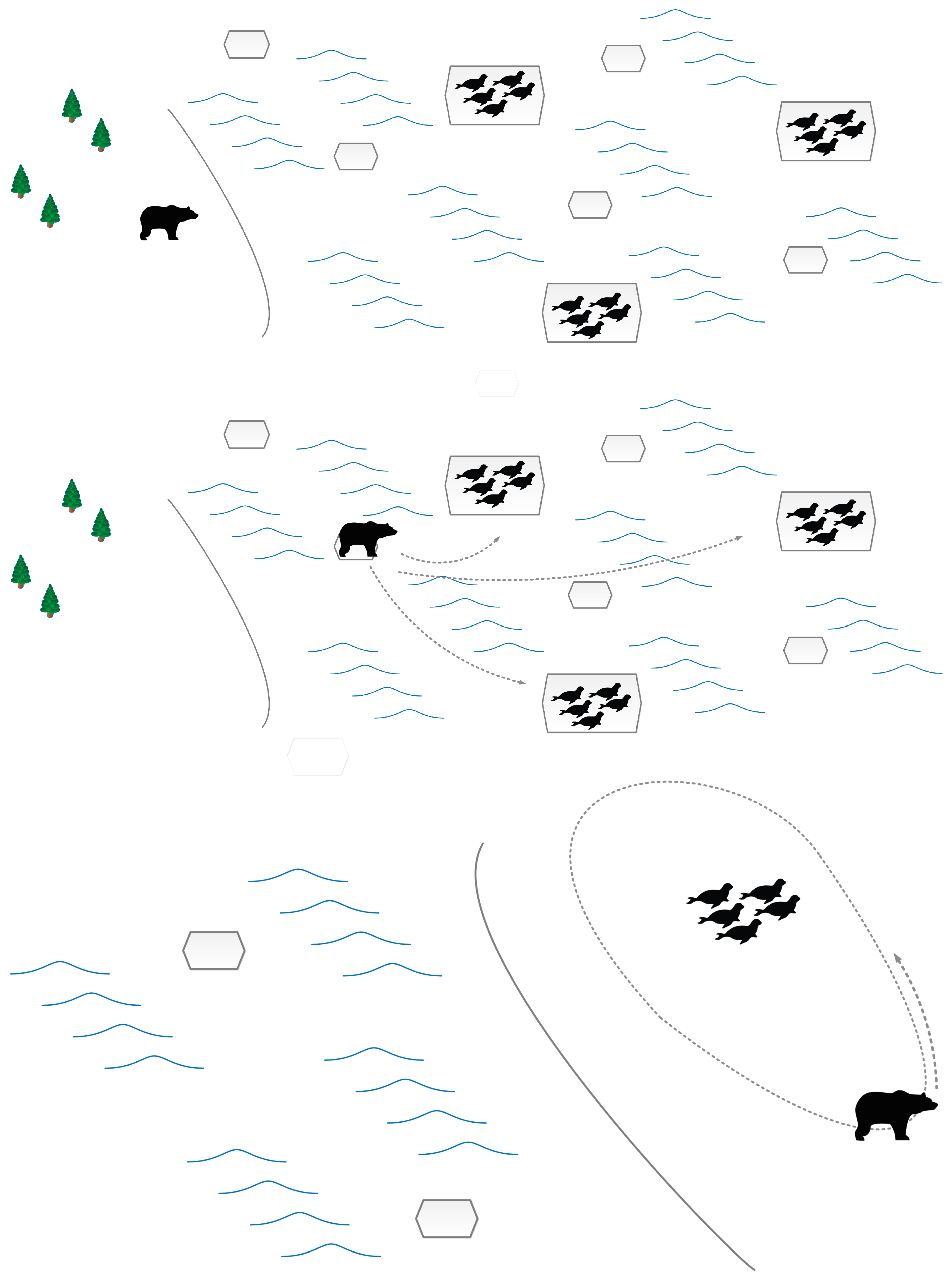
Figure 1.
Sample presentation of the behavior that we modeled into optimization strategy. Polar bear in his domain starts to search for possible seals colonies. To reach them polar bear must come across an arctic sea and land. He uses drifting ice floes to get to remote locations. When he finally spots the seals he tries to get closer without notice and surrounds the colony to choose the optimal prey.

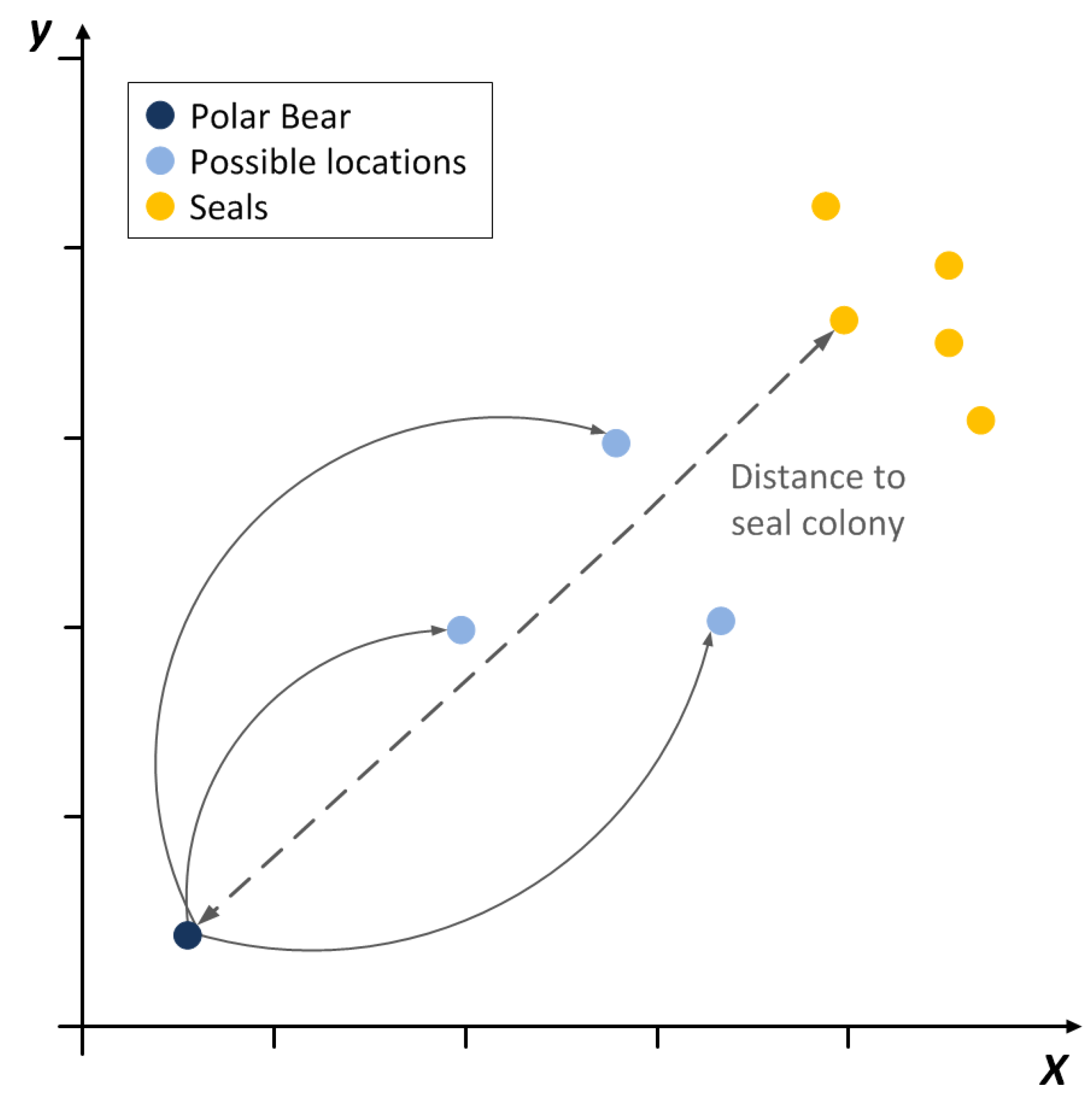
Figure 2.
PBO global search: Possible positions of polar bear while global movement on the ice floe in the search of seal habitats for hunting. Each individual moves toward the best position in the population by the use of proposed model.
Figure 2.
PBO global search: Possible positions of polar bear while global movement on the ice floe in the search of seal habitats for hunting. Each individual moves toward the best position in the population by the use of proposed model.

Figure 3.
PBO local search: Visualization of polar bear hunting movement in search for the best position to attack the seal on a 2D plane. The movement is modeled using modified single leaf of trifolium.
Figure 3.
PBO local search: Visualization of polar bear hunting movement in search for the best position to attack the seal on a 2D plane. The movement is modeled using modified single leaf of trifolium.

Figure 4.
Sample benchmark tests results for selected test functions from Table 1: Griewank, Rastragin, Rotated Hyper-Ellipsoid, Sphere, Sum squares, Zakharov, Schwefel : we can see a chart presenting each function in 2D, changes in the number of polar bears during optimization process, trajectory of the optimization representing average movement of individuals in the population, average fitness in the population, and convergence rate in the population.

Figure 5.
Scheme of pressure vessel model used to solve optimal design problem.
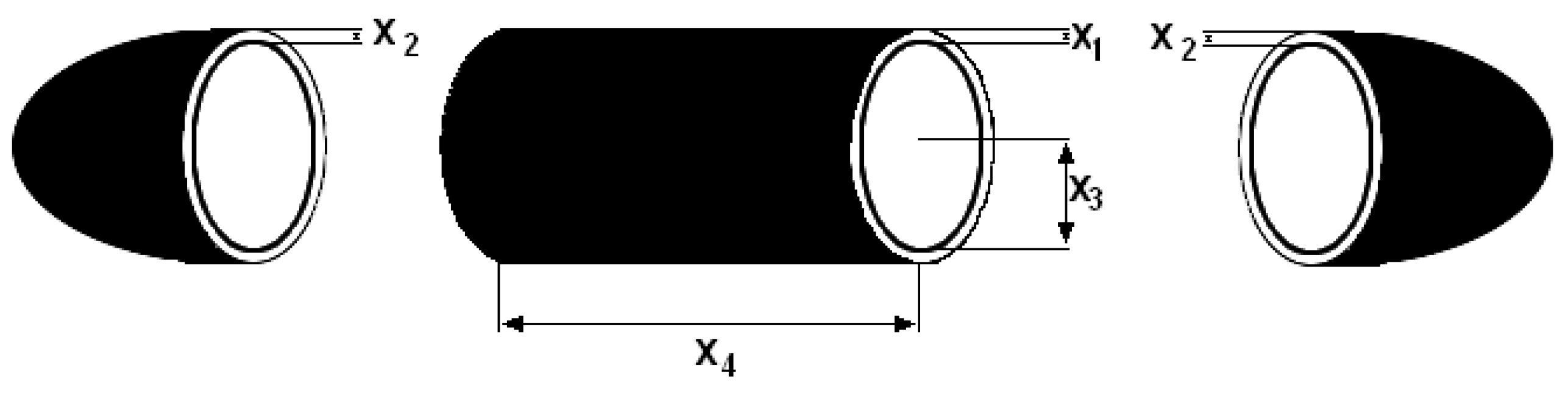
Figure 6.
Scheme of gear train model used to solve optimal design problem.

Figure 7.
Scheme of welded beam model used to solve optimal design problem.

Figure 8.
Scheme of compression spring model used to solve optimal design problem.

Table 1.
Benchmark test functions used in experimental verification.
| Function Name | Function f | Range | Solution | |
|---|---|---|---|---|
| Dixon-Price | 0 | |||
| Griewank | 0 | (0,…,0) | ||
| Powell | 0 | (0,…,0) | ||
| Rastragin | 0 | (0,…,0) | ||
| Rosenbrock | 0 | (1,…,1) | ||
| Hyper–Ellipsoid | 0 | (0,…,0) | ||
| Schwefel | 0 | (420.97,…,420.97) | ||
| Shubert | (0,…,0) | |||
| Sphere | 0 | (0,…,0) | ||
| Sum squares | 0 | (0,…,0) | ||
| Styblinski-Tang | (-2.9,…,-2.9) | |||
| Weierstrass | 0 | |||
| Zakharov | 0 | (0,…,0) |
Table 2.
Obtained optimal solutions for applied benchmark test functions, averaged for 100 results from performed benchmark tests.
Table 2.
Obtained optimal solutions for applied benchmark test functions, averaged for 100 results from performed benchmark tests.
| Function | BA | CSA | DA | FA | FPA | MFO | PBO | WWO | SA | GA | PSO | AACA |
|---|---|---|---|---|---|---|---|---|---|---|---|---|
| 0.00832 | 0.007718 | 0.007801 | 0.009989 | 0.008947 | 0.007517 | 0.007512 | 0.009713 | 0.007113 | 0.007621 | 0.007501 | 0.007613 | |
| 0.001837 | 0.000893 | 0.001092 | 0.002813 | 0.003815 | 0.000986 | 0.000052 | 0.000681 | 0.000102 | 0.000041 | 0.000052 | 0.000097 | |
| 0.001241 | 0.000874 | 0.00983 | 0.000873 | 0.000781 | 0.000208 | 0.000189 | 0.000198 | 0.000174 | 0.000321 | 0.000193 | 0.000202 | |
| 0.004602 | 0.004592 | 0.00513 | 0.005397 | 0.005284 | 0.004503 | 0.004483 | 0.003976 | 0.005612 | 0.004387 | 0.00404 | 0.005238 | |
| 0.030147 | 0.030281 | 0.029999 | 0.37326 | 0.033059 | 0.029193 | 0.27936 | 0.009826 | 0.008427 | 0.04356 | 0.02134 | 0.03243 | |
| 0.000981 | 0.000109 | 0.000087 | 0.000109 | 0.000054 | 0.000041 | 0.000039 | 0.007298 | 0.0002312 | 0.000074 | 0.000038 | 0.0003145 | |
| 0.04618 | 0.045801 | 0.041982 | 0.04784 | 0.046871 | 0.039982 | 0.04352 | 0.043891 | 0.0446127 | 0.0424365 | 0.038932 | 0.041324 | |
| −187.387 | −186.981 | −186.789 | −186.837 | −186.811 | −187.705 | −187.702 | −187.703 | −186.942 | −187.361 | −186.924 | −186.931 | |
| 0.001026 | 0.000866 | 0.000986 | 0.000872 | 0.000201 | 0.000132 | 0.000064 | 0.000127 | 0.000243 | 0.001103 | 0.000059 | 0.000124 | |
| 0.008765 | 0.002942 | 0.003856 | 0.004857 | 0.003927 | 0.000535 | 0.000289 | 0.008986 | 0.002476 | 0.003101 | 0.0004251 | 0.001621 | |
| −784.205 | −783.804 | −784.198 | −784.301 | −783.989 | −784.098 | −783.992 | −784.102 | −784.031 | −783.994 | −783.089 | −783.995 | |
| −0.50968 | −0.50991 | −0.51012 | −0.51830 | −0.52380 | −0.50910 | −0.50901 | −0.50992 | −0.59851 | −0.5312 | −0.50941 | −0.50993 | |
| 0.004972 | 0.00478 | 0.005629 | 0.007615 | 0.002371 | 0.000689 | 0.000683 | 0.000983 | 0.004351 | 0.006254 | 0.0006831 | 0.0007452 |
Table 3.
Standard deviation for obtained results for applied benchmark test functions.
| Function | BA | CSA | DA | FA | FPA | MFO | PBO | WWO | SA | GA | PSO | AACA |
|---|---|---|---|---|---|---|---|---|---|---|---|---|
Table 4.
p-values of the Wilcoxon rank-sum test for examined methods ( have been underlined).
| Function | BA | CSA | DA | FA | FPA | MFO | PBO | WWO | SA | GA | PSO | AACA |
|---|---|---|---|---|---|---|---|---|---|---|---|---|
| N/A | N/A | N/A | N/A | N/A | ||||||||
| N/A | N/A | N/A | N/A | |||||||||
| N/A | N/A | N/A | N/A | N/A | ||||||||
| N/A | N/A |
Table 5.
Optimal construction variables for the pressure vessel design problem.
| BA | CSA | DA | FA | FPA | MFO | PBO | WWO | SA | GA | PSO | AACA | |
|---|---|---|---|---|---|---|---|---|---|---|---|---|
| 0.81064 | 0.81958 | 0.81683 | 0.81082 | 0.82531 | 0.81738 | 0.81327 | 0.81038 | 0.81612 | 0.82034 | 0.81421 | 0.82313 | |
| 0.44675 | 0.44468 | 0.44721 | 0.49577 | 0.44466 | 0.43488 | 0.43702 | 0.43629 | 0.44115 | 0.44014 | 0.43611 | 0.44537 | |
| 42.15769 | 42.23808 | 42.14122 | 42.01106 | 42.15095 | 42.0162 | 42.04601 | 42.12014 | 42.10029 | 42.32500 | 42.13451 | 42.92300 | |
| 176.7288 | 176.87528 | 177.12321 | 177.69137 | 178.23268 | 176.9014 | 176.75597 | 177.96564 | 176.72880 | 176.43206 | 176.65122 | 176.73561 | |
| 6088.18314 | 6160.6034 | 6138.89315 | 6241.23766 | 6217.80235 | 6077.53166 | 6057.54657 | 6075.94324 | 6098.67000 | 6155.74048 | 6073.52853 | 6301.56641 |
Table 6.
Optimal variables for the gear train design problem.
| BA | CSA | DA | FA | FPA | MFO | PBO | WWO | SA | GA | PSO | AACA | |
|---|---|---|---|---|---|---|---|---|---|---|---|---|
| 57.4517 | 55.62869 | 52.44017 | 50.05234 | 51.15054 | 48.22301 | 50.04797 | 55.27473 | 51.34512 | 52.57125 | 51.32931 | 51.41824 | |
| 19.48176 | 16.71727 | 17.00267 | 24.38656 | 22.45769 | 18.77492 | 23.32433 | 24.3159 | 21.32743 | 23.19834 | 21.02347 | 21.35921 | |
| 18.58749 | 21.27387 | 22.99426 | 14.02798 | 17.97921 | 21.13716 | 14.82582 | 15.03104 | 14.98321 | 16.93254 | 14.79391 | 15.83209 | |
| 43.68715 | 44.31047 | 51.67159 | 46.3547 | 55.90958 | 57.03833 | 47.88919 | 45.82914 | 47.43271 | 48.24512 | 47.82131 | 47.34128 | |
| 1.53 × 10 | 3.09 × 10 | 3.02 × 10 | 6.52 × 10 | 4.83 × 10 | 1.44 × 10 | 1.37 × 10 | 5.67 × 10 | 1.71 × 10 | 1.13 × 10 | 3.08 × 10 | 2.87 × 10 |
Table 7.
Optimal variables for the welded beam design problem.
| BA | CSA | DA | FA | FPA | MFO | PBO | WWO | SA | GA | PSO | AACA | |
|---|---|---|---|---|---|---|---|---|---|---|---|---|
| 0.23848 | 0.22635 | 0.24685 | 0.25043 | 0.30209 | 0.21356 | 0.23258 | 0.25009 | 0.22413 | 0.22451 | 0.22131 | 0.22416 | |
| 3.48082 | 3.47836 | 3.477 | 3.69551 | 3.48829 | 3.49944 | 3.49706 | 3.7379 | 3.51812 | 3.49359 | 3.47241 | 3.51512 | |
| 8.71677 | 8.79874 | 8.56445 | 8.54958 | 8.98766 | 8.80996 | 8.91026 | 8.9735 | 8.64167 | 8.72150 | 8.65325 | 8.71412 | |
| 0.22242 | 0.21859 | 0.24589 | 0.2787 | 0.24566 | 0.21283 | 0.21194 | 0.22149 | 0.25139 | 0.22451 | 0.21312 | 0.23151 | |
| 1.84923 | 1.81413 | 2.00481 | 2.28456 | 2.20932 | 1.7549 | 1.79863 | 1.95437 | 2.02615 | 1.84247 | 1.73809 | 1.89509 |
Table 8.
Optimal variables for the compression spring design problem.
| BA | CSA | DA | FA | FPA | MFO | PBO | WWO | SA | GA | PSO | AACA | |
|---|---|---|---|---|---|---|---|---|---|---|---|---|
| 0.05231 | 0.05242 | 0.05214 | 0.05253 | |||||||||
| 0.34412 | 0.35325 | 0.34346 | 0.34512 | |||||||||
| 11.62350 | 11.68242 | 11.62233 | 11.63542 | |||||||||
| 0.01283 | 0.01328 | 0.01272 | 0.01299 |
© 2017 by the authors. Licensee MDPI, Basel, Switzerland. This article is an open access article distributed under the terms and conditions of the Creative Commons Attribution (CC BY) license (http://creativecommons.org/licenses/by/4.0/).
Share and Cite
MDPI and ACS Style
Połap, D.; Woz´niak, M. Polar Bear Optimization Algorithm: Meta-Heuristic with Fast Population Movement and Dynamic Birth and Death Mechanism. Symmetry 2017, 9, 203. https://doi.org/10.3390/sym9100203
AMA Style
Połap D, Woz´niak M. Polar Bear Optimization Algorithm: Meta-Heuristic with Fast Population Movement and Dynamic Birth and Death Mechanism. Symmetry. 2017; 9(10):203. https://doi.org/10.3390/sym9100203
Chicago/Turabian StylePołap, Dawid, and Marcin Woz´niak. 2017. "Polar Bear Optimization Algorithm: Meta-Heuristic with Fast Population Movement and Dynamic Birth and Death Mechanism" Symmetry 9, no. 10: 203. https://doi.org/10.3390/sym9100203
Note that from the first issue of 2016, this journal uses article numbers instead of page numbers. See further details here.