
ANFIS-Based Modeling for Photovoltaic Characteristics Estimation

Abstract
:
1. Introduction
2. ANFIS and PV Modeling
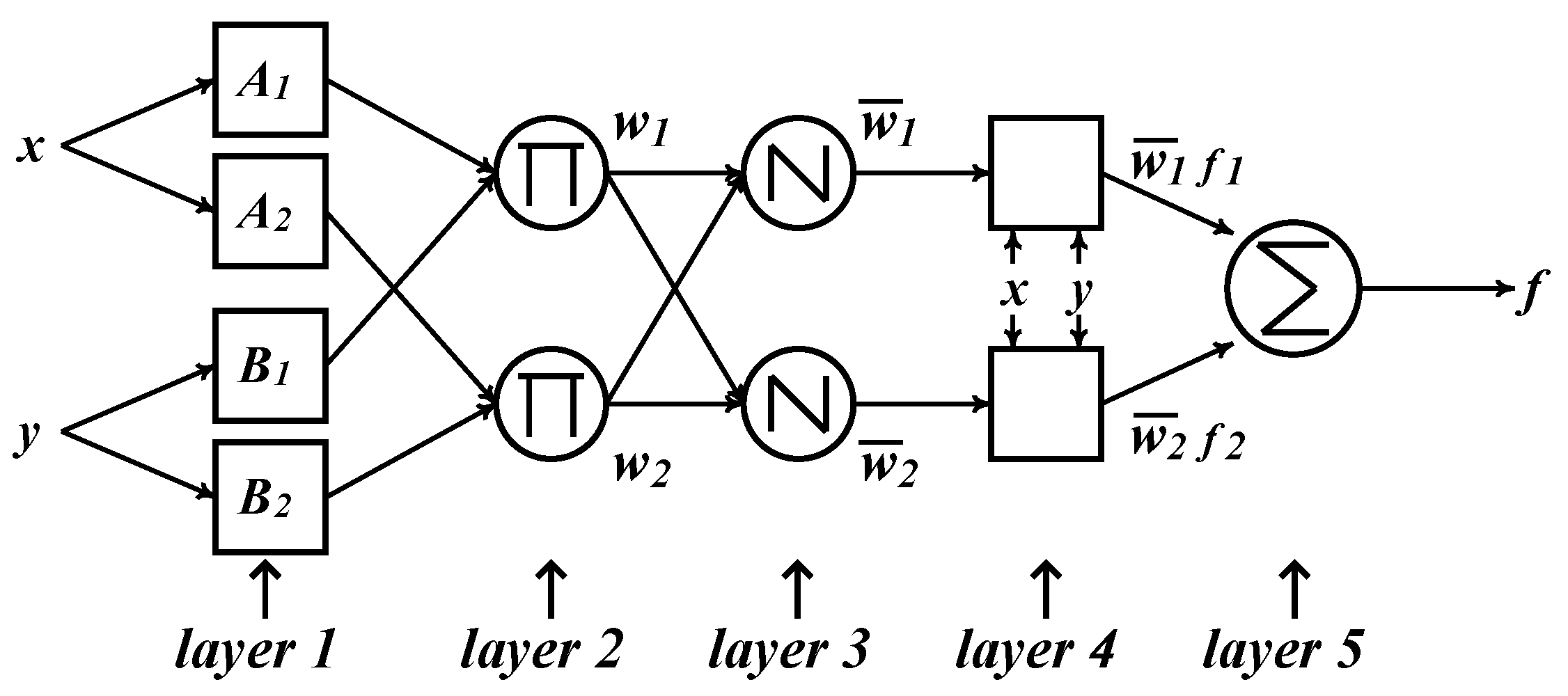
2.1. ANFIS
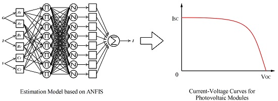
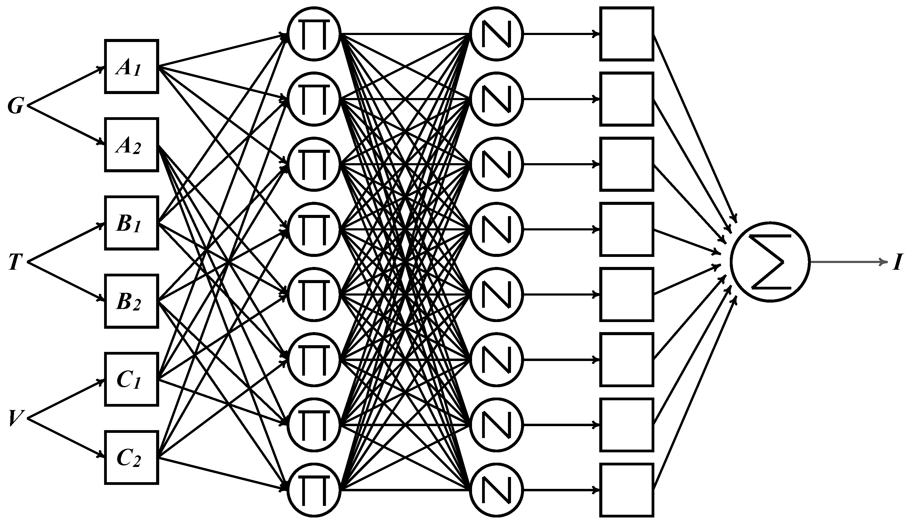
2.2. The Proposed PV Model
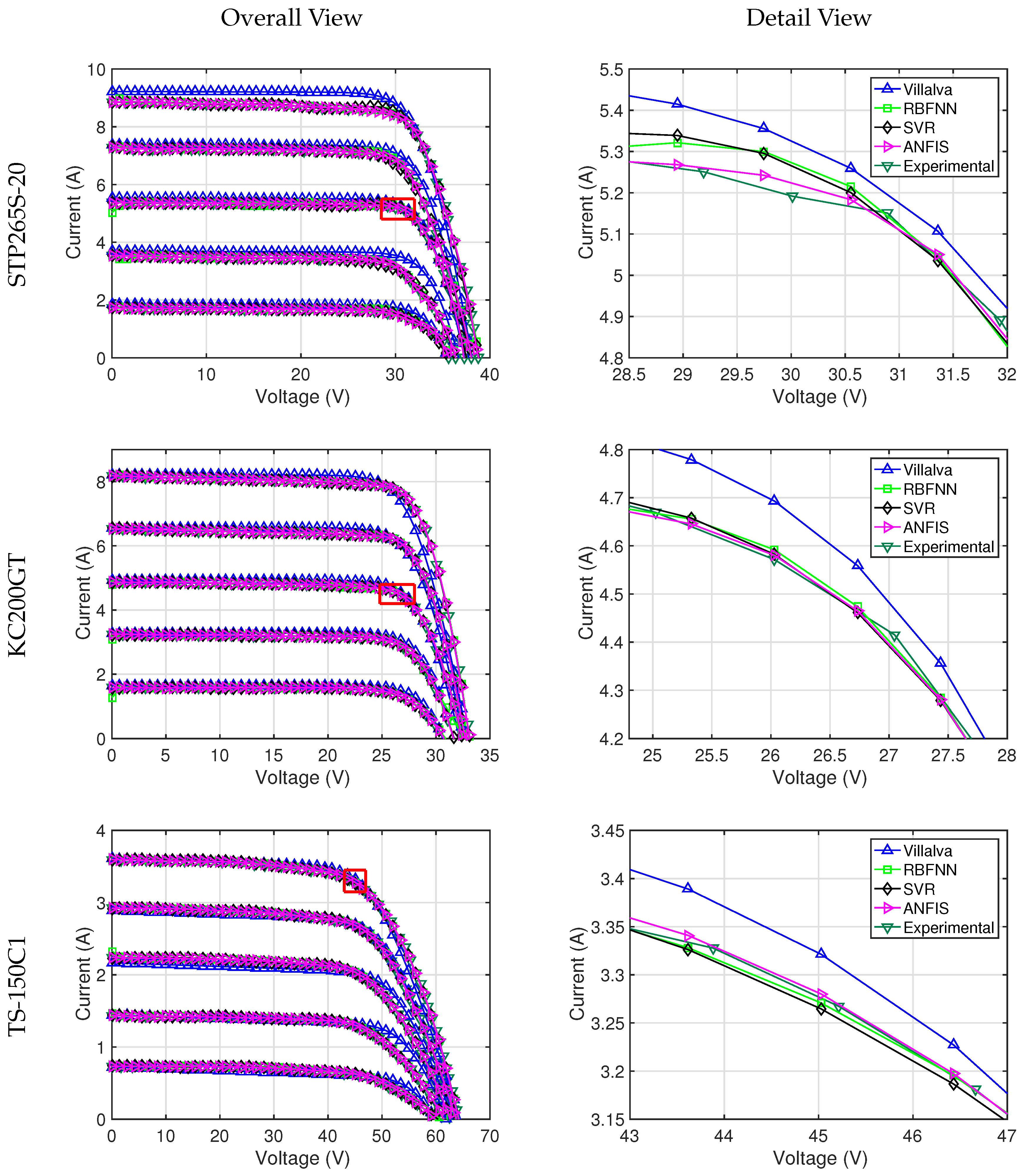
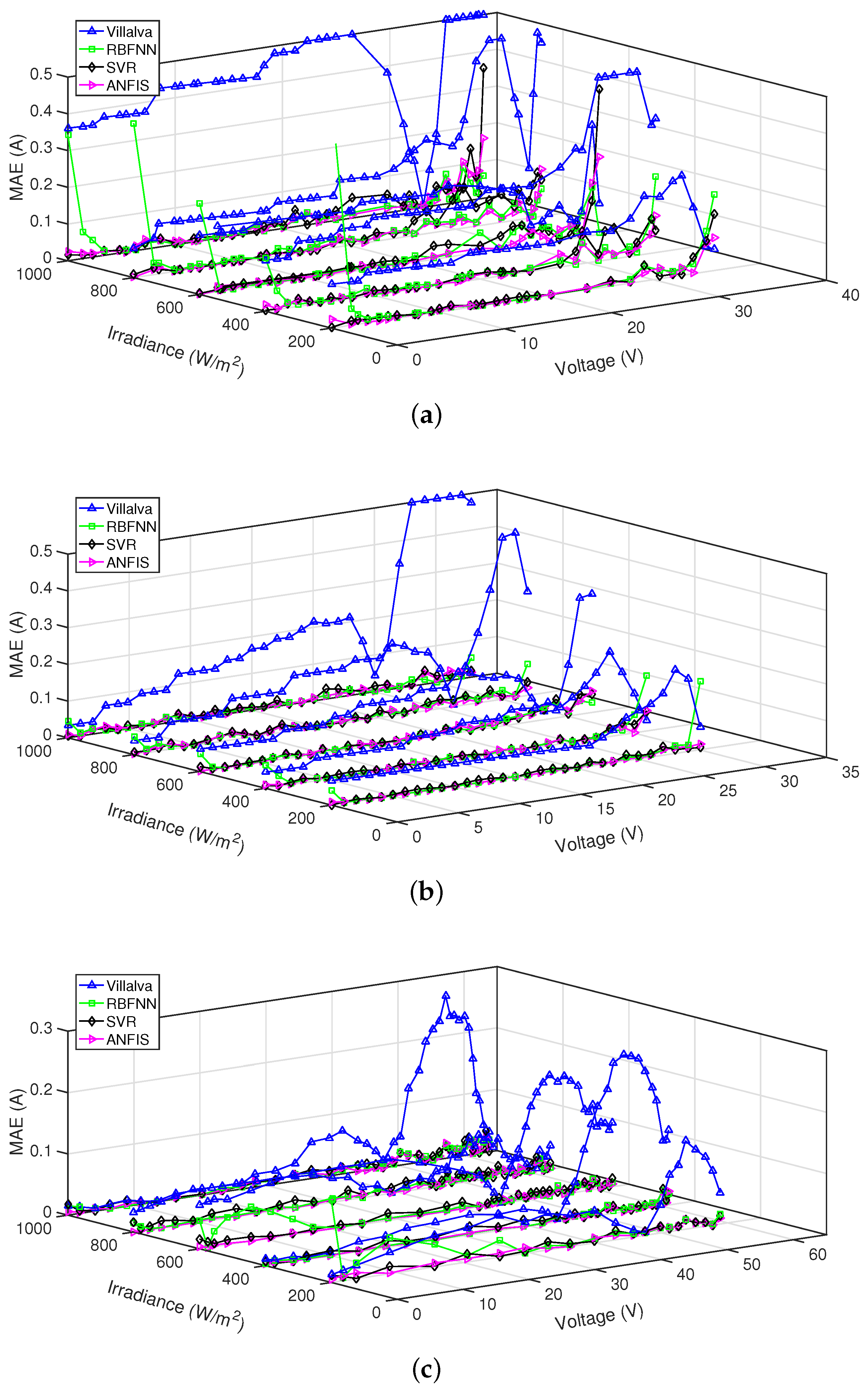
3. Results
4. Conclusions
Acknowledgments
Author Contributions
Conflicts of Interest
Abbreviations
| AM | air mass |
| maximum power (W) | |
| open circuit voltage (V) | |
| short circuit current (A) | |
| maximum power point voltage (V) | |
| maximum power point current (A) | |
| temperature coefficients of open circuit voltage (V/K) | |
| temperature coefficients of short circuit current (A/K) | |
| number of cells in series |
References
- Chin, V.J.; Salam, Z.; Ishaque, K. Cell modelling and model parameters estimation techniques for photovoltaic simulator application: A review. Appl. Energy 2015, 154, 500–519. [Google Scholar] [CrossRef]
- Brano, V.L.; Orioli, A.; Ciulla, G.; Gangi, A.D. An improved five-parameter model for photovoltaic modules. Sol. Energy Mater. Sol. Cells 2010, 94, 1358–1370. [Google Scholar] [CrossRef]
- Brano, V.L.; Orioli, A.; Ciulla, G. On the experimental validation of an improved five-parameter model for silicon photovoltaic modules. Sol. Energy Mater. Sol. Cells 2012, 102, 27–39. [Google Scholar] [CrossRef]
- Ma, J.; Ting, T.O.; Man, K.L.; Zhang, N.; Guan, S.U.; Wong, P.W.H. Parameter estimation of photovoltaic models via cuckoo search. J. Appl. Math. 2013, 2013, 362619. [Google Scholar] [CrossRef]
- Piazza, M.C.D.; Pucci, M.; Ragusa, A.; Vitale, G. Analytical Versus Neural Real-Time Simulation of a Photovoltaic Generator Based on a DC–DC Converter. IEEE Trans. Ind. Appl. 2010, 46, 2501–2510. [Google Scholar] [CrossRef]
- Villalva, M.G.; Gazoli, J.R.; Filho, E.R. Comprehensive approach to modeling and simulation of photovoltaic arrays. IEEE Trans. Power Electron. 2009, 24, 1198–1208. [Google Scholar] [CrossRef]
- Salam, Z.; Ishaque, K.; Taheri, H. An improved two-diode Photo-voltaic (PV) model for PV system. In Proceedings of the 2010 Joint International Conference on Power Electronics, Drives and Energy Systems (PEDES) and 2010 Power India, New Delhi, India, 20–23 December 2010; pp. 1–5.
- Chan, D.S.H.; Phang, J.C.H. Analytical methods for the extraction of solar-cell single- and double-diode model parameters from I-V characteristics. IEEE Trans. Electron Devices 1987, 34, 286–293. [Google Scholar] [CrossRef]
- Laudani, A.; Fulginei, F.R.; Salvini, A. High performing extraction procedure for the one-diode model of a photovoltaic panel from experimental I-V curves by using reduced forms. Sol. Energy 2014, 103, 316–326. [Google Scholar] [CrossRef]
- Laudani, A.; Fulginei, F.R.; Salvini, A. Identification of the one-diode model for photovoltaic modules from datasheet values. Sol. Energy 2014, 108, 432–446. [Google Scholar] [CrossRef]
- Mahmoud, Y.A.; Xiao, W.; Zeineldin, H.H. A parameterization approach for enhancing PV model accuracy. IEEE Trans. Ind. Electron. 2013, 60, 5708–5716. [Google Scholar] [CrossRef]
- Mashaly, H.M.; Sharaf, A.M.; Mansour, M.; El-Sattar, A.A. A photovoltaic maximum power tracking scheme using neural networks. In Proceedings of the 3rd IEEE Conference on Control Applications, Glasgow, UK, 24–26 August 1994; Volume 1, pp. 160–172.
- Hiyama, T. Identification of optimal operating point of PV modules using neural network for real time maximum power tracking control. IEEE Trans. Energy Convers. 1995, 10, 360–367. [Google Scholar] [CrossRef]
- Al-Amoudi, A.; Zhang, L. Application of radial basis function networks for solar- array modelling and maximum power-point prediction. IEEE Proc. Gener. Transm. Distrib. 2000, 147, 310–316. [Google Scholar] [CrossRef]
- Zhang, L.; Bai, Y.F. Genetic algorithm-trained radial basis function neural networks for modelling photovoltaic panels. Eng. Appl. Artif. Intell. 2005, 18, 833–844. [Google Scholar] [CrossRef]
- Bonanno, F.; Capizzi, G.; Graditi, G.; Napoli, C.; Tina, G.M. A radial basis function neural network based approach for the electrical characteristics estimation of a photovoltaic module. Appl. Energy 2012, 97, 956–961. [Google Scholar] [CrossRef]
- Shi, J.; Lee, W.J.; Liu, Y.; Yang, Y.; Wang, P. Forecasting power output of photovoltaic system based on weather classification and support vector machines. IEEE Trans. Ind. Appl. 2012, 48, 1064–1069. [Google Scholar] [CrossRef]
- Drucker, H.; Burges, C.J.C.; Kaufman, L.; Smola, A.; Vapnik, V. Support vector regression machines. Adv. Neural Inf. Process Syst. 1996, 28, 779–784. [Google Scholar]
- Jang, J.R. ANFIS: Adaptive-network-based fuzzy inference system. IEEE Trans. Syst. Man Cybern. 1993, 23, 665–685. [Google Scholar] [CrossRef]
- Kharb, R.K.; Shimi, S.L.; Chatterji, S.; Ansari, M.F. Modeling of solar PV module and maximum power point tracking using ANFIS. Renew. Sustain. Energy Rev. 2014, 33, 602–612. [Google Scholar] [CrossRef]
- Sharma, R.; Patterh, M.S. A new pose invariant face recognition system using PCA and ANFIS. Optik 2015, 126, 3483–3487. [Google Scholar] [CrossRef]
- Choi, I.H.; Pak, J.M.; Ahn, C.K.; Lee, S.H.; Lim, M.T.; Song, M.K. Arbitration algorithm of FIR filter and optical flow based on ANFIS for visual object tracking. Measurement 2015, 75, 338–353. [Google Scholar] [CrossRef]
- Chang, C.C.; Lin, C.J. LIBSVM : A library for support vector machines. ACM Trans. Intell. Syst. Tech. 2011, 2. [Google Scholar] [CrossRef]


| Module | STP265S-20 | KC200GT | TS-150C1 |
|---|---|---|---|
| Technology | mono-crystalline | poly-crystalline | thin-film |
| (W) | 265.05 | 200.14 | 149.96 |
| (V) | 38.1 | 32.9 | 64.5 |
| (A) | 9.22 | 8.21 | 3.61 |
| (V) | 30.5 | 26.3 | 46.0 |
| (A) | 8.69 | 7.61 | 3.26 |
| (V/K) | −0.130 | −0.123 | −0.187 |
| (A/K) | 5.53 × 10 | 3.18 × 10 | 3.61 × 10 |
| 60 | 54 | 100 |
| Method | STP265S-20 | KC200GT | TS-150C1 | ||||||
|---|---|---|---|---|---|---|---|---|---|
| RMSE | MAPE | R (%) | RMSE | MAPE | R (%) | RMSE | MAPE | R (%) | |
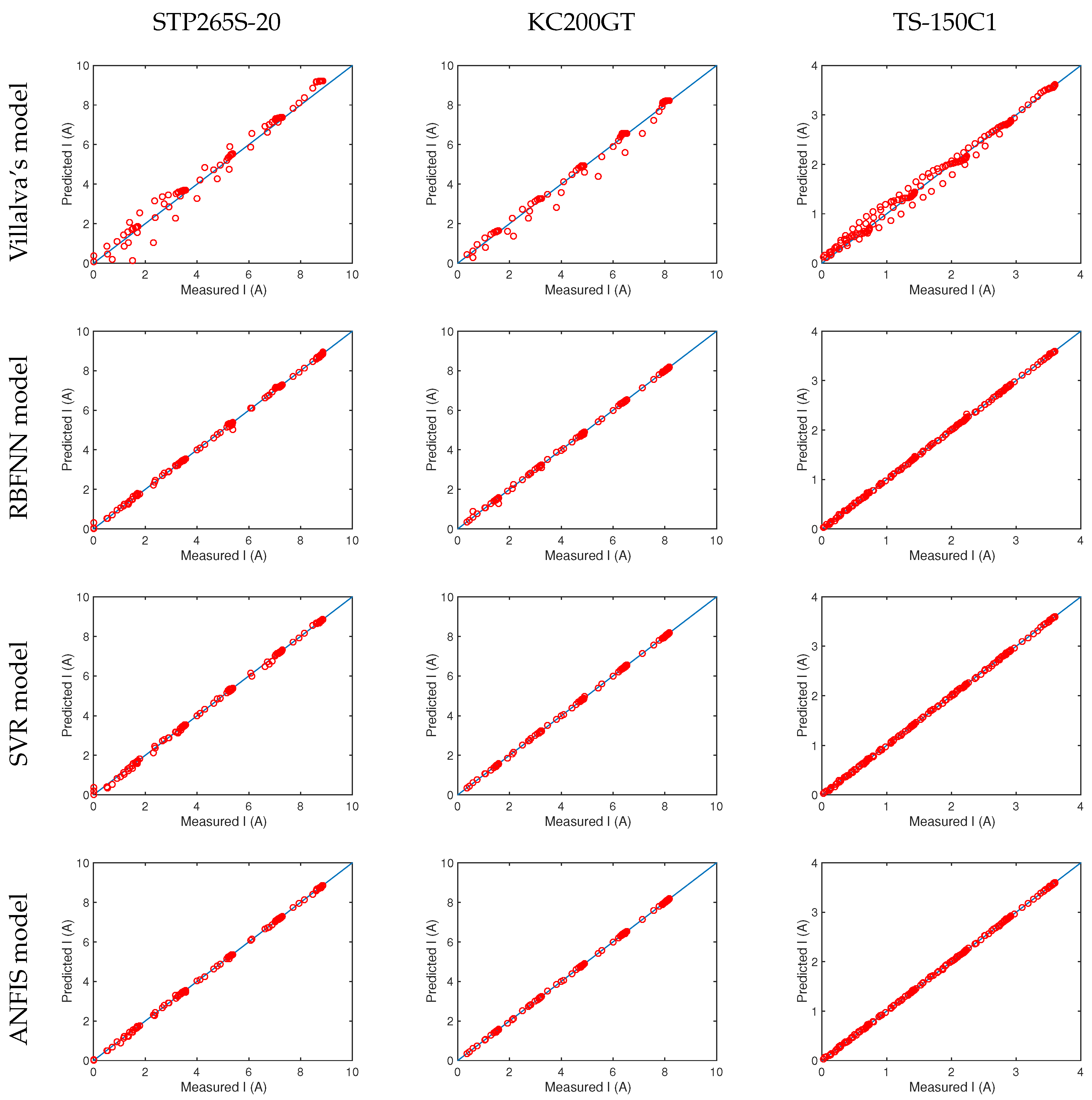
| Villalva’s model [6] | 0.6754 | 11.859 | 94.50 | 0.2032 | 0.0499 | 99.27 | 0.1007 | 0.1386 | 99.04 |
| RBFNN model * | 0.0458 | 1.9232 | 99.97 | 0.0381 | 0.0071 | 99.97 | 0.0414 | 0.0204 | 99.71 |
| SVR model | 0.0574 | 3.1932 | 99.95 | 0.0145 | 0.0037 | 99.99 | 0.0105 | 0.0150 | 99.99 |
| ANFIS model | 0.0280 | 0.7363 | 99.99 | 0.0123 | 0.0026 | 99.99 | 0.0079 | 0.0109 | 99.99 |
© 2016 by the authors; licensee MDPI, Basel, Switzerland. This article is an open access article distributed under the terms and conditions of the Creative Commons Attribution (CC-BY) license (http://creativecommons.org/licenses/by/4.0/).
Share and Cite
Bi, Z.; Ma, J.; Pan, X.; Wang, J.; Shi, Y. ANFIS-Based Modeling for Photovoltaic Characteristics Estimation. Symmetry 2016, 8, 96. https://doi.org/10.3390/sym8090096
Bi Z, Ma J, Pan X, Wang J, Shi Y. ANFIS-Based Modeling for Photovoltaic Characteristics Estimation. Symmetry. 2016; 8(9):96. https://doi.org/10.3390/sym8090096
Chicago/Turabian StyleBi, Ziqiang, Jieming Ma, Xinyu Pan, Jian Wang, and Yu Shi. 2016. "ANFIS-Based Modeling for Photovoltaic Characteristics Estimation" Symmetry 8, no. 9: 96. https://doi.org/10.3390/sym8090096