Polarity Formation in Molecular Crystals as a Symmetry Breaking Effect

Abstract

The transition of molecular crystals into a polar state is modeled by a one-dimensional Ising Hamiltonian in multipole expansion and a suitable order parameter. Two symmetry breakings are necessary for the transition: the translational and the spin flip invariance—the former being broken by geometric constraints, the latter by the interaction of the first non-zero multipole with the next order multipole. Two different behaviors of the thermal average of the order parameter as a function of position are found. The free energy per lattice site converges to a finite value in the thermodynamic limit showing the consistency of the model in a macroscopic representation.

1. Introduction

Polar molecules located at lattice sites as found in molecular crystals represent a system to discuss the effects of symmetry breaking in the statistical calculation of a property such as electrical polarity. Given the point symmetry of the lattice and its finite size, the system will thermalize into a bi-polar state featuring zero overall polarity [1].

Starting from our previous work [2], we consider a generalized Ising model whose Hamiltonian is given as an infinite series of multipoles. The well known spin flip symmetry of the Ising Hamiltonian is found to be broken by the interaction of the first non-zero multipole with the next order multipole, when such an interaction is present. This is analogous to the effect of an external magnetic field acting on a paramagnetic system where the symmetry breaking in the Hamiltonian generates an induced magnetization in the material. As a result of the coupling of the symmetry breaking in the Hamiltonian with the translational symmetry breaking due to the free boundary conditions, a spatial ordering in the system is achieved.

2. Ising Model for Bi-Polar Transition

The simplest model one can imagine to reproduce bi-polar state formation in media is an Ising-like one. It consists in a three-dimensional cubic lattice Γ and the binary variables $S_i=\pm 1$ defined on each of its site i. Only interaction between neighboring variables are included. The energy of a given configuration $\left\{S_i\right\}$ is given by the Ising Hamiltonian

$$-H=J\sum _{\langle i,j\rangle }{S}_i{S}_j,$$

(1)

where the symbol $\langle i,j\rangle$ indicates that the sum is between the next neighboring $S_i$ only. Since the Hamiltonian (1) is invariant under the transformation $S_i\to -S_i$, $S_j\to -S_j$ (global spin flip symmetry) the thermal average $\langle S_i\rangle =0$, unless this symmetry is broken. Thus, Equation (1), in this simple form, cannot reproduce a net average polarity. In order to analyze the issue in more detail, consider two non-overlapping charge distributions centered around ${\mathbf{R}}_{\mathbf{A}}$ and ${\mathbf{R}}_{\mathbf{B}}$, respectively. The electrostatic energy in multipole expansion can be written as:

$$V\left(R_{AB}\right)=k_C\sum _{l_A=0}^{\infty }\sum _{l_B=0}^{\infty }{(-1)}^{l_B},{\left(Q_A\right)}_{l_A}{B}^{l_A,l_B}{\left(Q_B\right)}_{l_B},$$

(2)

where ${\mathbf{R}}_{\mathbf{AB}}={\mathbf{R}}_{\mathbf{B}}-{\mathbf{R}}_{\mathbf{A}}$, $k_C$ is the Coulomb constant whose value depends on the units, and where for each $l_A$, $l_B$ $\in (0,\infty )$ the $(2l_A+1)\times (2l_B+1)$ matrix $B^{l_A,l_B}$ is defined as

$$B_{m_A,m_B}^{l_A,l_B}={\left(\genfrac{}{}{0pt}{}{2(l_A+l_B)}{2l_A}\right)}^{1/2}{(-1)}^{m_A+m_B}{I}_{l_A+l_B}^{-(m_A+m_B)}\left({\mathbf{R}}_{\mathbf{AB}}\right)C_{l_A{m}_A,l_B{m}_B}^{l_A+l_B}|m_A|\le l_A,\left|m_B\right|\le l_B,$$

(3)

where $I_l^m\left(r\right)$ are the irregular solid harmonics, $C_{l_A{m}_A,l_B{m}_B}^{l_A+l_B}$ are the Clebsch–Gordan coefficients. and ${\left(Q_A\right)}_l^m$ (resp. ${\left(Q_B\right)}_l^m)$ are the multipole moments of distribution A (resp. B) given by

$$Q_l^m=\sum _i^N{q}_i{R}_l^m\left({\mathbf{r}}_{\mathbf{i}}\right),$$

(4)

where ${\mathbf{r}}_{\mathbf{i}}$ is the position of the charge $q_i$ of the distribution considered, and $R_l^m\left(r_i\right)$ are the regular solid harmonics. Since the $Q_l^m$ have parity ${(-1)}^l$ $\forall m$, it turns out that each term in the sum of Equation (2) has a well definite parity. The interactions of multipoles such that $l_A+l_B$ is odd are, therefore, the origin of the symmetry breaking in Equation (1). This condition is, however, not sufficient for the onset of a bi-polar state because, as we will show in the following, the translational symmetry of the system should also be broken in one direction at least. This is not surprising as in the thermodynamic limit we need to have a "free" (of interaction from the outside) surface where the bi-polar state shows up.

According to the above discussion, if the system has a net charge, the lowest order terms of the series Equation (2) with broken (parity) symmetry are those with $l_A=0$, $l_B=1$ and $l_A=1$, $l_B=0$, which correspond to charge-dipole interactions. If the system is electrically neutral but polar, the symmetry is broken by the dipole-quadrupole interactions, at lowest order.

Let us consider a one-dimensional array of N identical molecules located at the sites i of the lattice and assume that each molecule i can be in one of the two possible states $S_i$ differing by an overall rotation of 180${}^{\circ }$ around the center of mass, i.e., an inversion of the dipolar direction. The multipole moments will, in general, be dependent on the state of the molecule according to some relation of the kind:

$$Q_{i,l}^m=S_i^l{q}_l^m,$$

(5)

where the $q_l^m$ are the multipole moments of molecule i in a reference state arbitrarily chosen for all molecules, $S_i^l$ is the usual effective “spin” variable associated to molecule i to the power of l. Due to the parity symmetry, only l-odded multipoles are affected by molecule flip.

The Ising Hamiltonian (1) can be re-written as

$$H=\sum _{\langle i,j\rangle }\sum _{l_i=0}^{\infty }\sum _{l_j=0}^{\infty }{S}_i^{l_i}{S}_j^{l_j}{A}_{l_i,l_j},$$

(6)

where $A_{l_i,l_j}$ are given by

$$A_{l_i,l_j}=k_C{(-1)}^{l_j}{B}_{m_i,m_j}^{l_A,l_B}.$$

(7)

It is straightforward to see that the transformation $\{l_i,m_i\}⟷\{l_j,m_j\}$ gives $A_{l_i,l_j}={(-1)}^{l_i+l_j}{A}_{l_j,l_i}$, and, therefore, the matrix of interactions has parity $l_i+l_j$. The diagonal terms $A_{l_i,l_i}$ can be expressed in the more compact form

$$A_{l,l}=k_C{(-1)}^l{q}_l{B}^l{q}_l,$$

(8)

where, for each $l\in (0,\infty )$,

$$B_{m_i,m_j}^l={\left(\genfrac{}{}{0pt}{}{4l}{2l}\right)}^{1/2}{(-1)}^{m_i+m_j}{I}_{2l}^{-(m_i+m_j)}\left({\mathbf{R}}_{\mathbf{ij}}\right)C_{l{m}_i,l{m}_j}^{2l}{m}_i,m_j=-l,\cdots l.$$

(9)

By using the symmetry properties of the Clebsch–Gordan coefficients, it can easily be seen that $B^l$ is symmetric $\forall l\in (0,\infty )$. For one-dimensional lattices, the matrices $B^l$ are of a particular simple form. Let us assume that the lattice extends over the z-axis, from the symmetry of the spherical harmonics and of the Clebsch–Gordan coefficients, we then get

$$B_{m_i,m_j}^l=\frac{\left(2l\right)!}{(l-m_i)!(l+m_i)!}{I}_{2l}^0\left(R_{ij}\right){\delta }_{m_i+m_j,0}{m}_i,m_j=-l,\cdots l,$$

(10)

which, for each l, is an anti-diagonal matrix.

To highlight the properties of the Hamiltonian let us separate the sums in Equation (6) over odd and even $l_i$ and $l_j$

$$H=\sum _{\langle i,j\rangle }\left[{\sum _{l_i,l_j}}^g{A}_{l_i,l_j}{S}_i^{l_i}{S}_j^{l_j}+{\sum _{l_i}}^g{\sum _{l_i}}^u{A}_{l_i,l_j}{S}_i^{l_i}{S}_j^{l_j}+{\sum _{l_i}}^u{\sum _{l_i}}^g{A}_{l_i,l_j}{S}_i^{l_i}{S}_j^{l_j}+{\sum _{l_i,l_j}}^u{A}_{l_i,l_j}{S}_i^{l_i}{S}_j^{l_j}\right],$$

(11)

where the superscript g (resp. u) indicates that the corresponding sum runs over the even (resp. odd) indices. Using the definition of $S_i$, the previous Equation simplifies to give

$$H=(N-1){\sum _{l_i,l_j}}^g{A}_{l_i,l_j}+{\sum _{l_i}}^g{\sum _{l_j}}^u{A}_{l_i,l_j}{S}_1+{\sum _{l_i}}^u{\sum _{l_j}}^g{A}_{l_i,l_j}{S}_N+\sum _{\langle i,j\rangle }{\sum _{l_i,l_j}}^u{A}_{l_i,l_j}{S}_i{S}_j,$$

(12)

and after swapping the index in the third sum and using the rule of transformation for $A_{l_i,l_j}$, we finally get

$$H=(N-1){\sum _{l_i,l_j}}^g{A}_{l_i,l_j}+(S_1-S_N){\sum _{l_i}}^g{\sum _{l_j}}^u{A}_{l_i,l_j}+\sum _{\langle i,j\rangle }{\sum _{l_i,l_j}}^u{A}_{l_i,l_j}{S}_i{S}_j.$$

(13)

In respect to the $S_i$ variables, the Hamiltonian is therefore decomposed into the sum of three terms: one is a constant, one anti-symmetric and one symmetric

$$H=const.+H_{\mathrm{u}}+H_{\mathrm{g}},$$

(14)

where

$$\begin{array}{ccc}{H}_{\mathrm{u}}\hfill & =& (S_1-S_N){\displaystyle {\sum _{l_i}}^g{\sum _{l_j}}^u{A}_{l_i,l_j}},\hfill \\ H_{\mathrm{g}}\hfill & =& {\displaystyle \sum _{\langle i,j\rangle }{\sum _{l_i,l_j}}^u{A}_{l_i,l_j}{S}_i{S}_j}.\hfill \end{array}$$

(15)

Note that $H_g$ is the usual Ising Hamiltonian with coupling constants given by

$$J_{ij}=-{\sum _{l_i,l_j}}^u{A}_{l_i,l_j},$$

(16)

and, therefore, it is the same Hamiltonian as an Ising ferromagnetic or anti-ferromagnetic depending on the sign of the $J_{ij}$s.

2.1. First Order Expansion

Even if, as a matter of fact, crystals are grown with neutral molecules, we consider here the first order expansion of charged molecules because, in spite of its simplicity, it contains the fundamental ingredients accounting for symmetry breaking. The more general case of second order will be treated in the next section. The first order coefficients Equation (7) are

$$\begin{array}{ccc}{A}_{0,0}\hfill & =& k_C{I}_0^0\left({\mathbf{R}}_{\mathbf{ij}}\right)q_0^0{q}_0^0{C}_{00,00}^0,\hfill \\ A_{0,1}\hfill & =& -k_C{q}_0{B}^{0,1}{q}_1{C}_{00,1m_j}^1,\hfill \\ A_{1,0}\hfill & =& -A_{1,0},\hfill \\ A_{1,1}\hfill & =& -k_C{q}_1{B}^1{q}_1.\hfill \end{array}$$

(17)

In Cartesian coordinates, with the z-axis assumed along the lattice, it is straightforward to recognize that $A_{0,0}=k_c{q}_{tot}^2/z^2$, $A_{0,1}=-k_C{q}_{tot}{p}_z/z^3$, $A_{1,0}=-A_{0,1}$ and $A_{1,1}=-2k_C{p}_z^2/z^3$ are the energies of a charge-charge, charge-dipole, dipole-charge and dipole-dipole Coulomb interactions, respectively. In the previous formulas, we have denoted by $q_{tot}$ the total charge of the molecule and with $p_z$ the z-component of the dipole moment (up to the sign) of the molecule.

Finally, the Hamiltonian (13), at the first order approximation, can be expressed as:

$$\begin{array}{ccc}{\mathcal{H}}^{\left(1\right)}\hfill & =& A_{0,0}(N-1)+A_{1,0}\sum _{\langle i,j\rangle }{S}_i-A_{1,0}\sum _{\langle i,j\rangle }{S}_j+A_{1,1}\sum _{\langle i,j\rangle }{S}_i{S}_j=\hfill \\ & =& A_{0,0}(N-1)+A_{1,0}(S_1-S_N)+A_{1,1}\sum _{\langle i,j\rangle }{S}_i{S}_j\hfill \end{array}.$$

(18)

2.2. Second Order Expansion

Let us turn ourselves to the more frequent situation of neutral molecules with non-zero first order moment. In addition to Equation (17), we need the second order interaction coefficients given by:

$$\begin{array}{ccc}{A}_{2,0}\hfill & =& A_{0,2}=0,\hfill \\ A_{2,1}\hfill & =& -A_{1,2}=-k_C{q}_2{B}^{2,1}{q}_1,\hfill \\ A_{2,2}\hfill & =& k_C{q}_2{B}^2{q}_2.\hfill \end{array}$$

(19)

The second order Hamiltonian is given by

$${\mathcal{H}}^{\left(2\right)}={\mathcal{H}}^{\left(1\right)}+A_{2,1}\sum _{\langle i,j\rangle }{S}_i+A_{1,2}\sum _{\langle i,j\rangle }{S}_j+A_{2,2}(N-1).$$

(20)

Equation (18) for neutral molecules reduces to ${\mathcal{H}}^{\left(1\right)}=A_{1,1}{\sum }_{\langle i,j\rangle }{S}_i{S}_j$. Note that the neutrality of the molecule restores the parity invariance of the Hamiltonian at a first order approximation. By inserting ${\mathcal{H}}^{\left(1\right)}$ in the expression for ${\mathcal{H}}^{\left(2\right)}$, and after minor manipulations, we finally get

$${\mathcal{H}}^{\left(2\right)}=A_{1,1}\sum _{\langle i,j\rangle }{S}_i{S}_j+A_{2,1}(S_1-S_N)+A_{2,2}(N-1).$$

(21)

This expression is formally equivalent to the Hamiltonian introduced by Bebie and Hulliger [2], with the position

$$\begin{array}{ccc}{A}_{1,1}\hfill & =& -(E_{\mathrm{AA}}+E_{\mathrm{DD}}-2E_{\mathrm{AD}})/4,\hfill \\ A_{2,1}\hfill & =& (E_{\mathrm{AA}}-E_{\mathrm{DD}})/4,\hfill \\ A_{2,2}\hfill & =& 2E_{\mathrm{A}D}+E_{\mathrm{D}D}+E_{\mathrm{AA}},\hfill \end{array}$$

(22)

where $E_{\mathrm{AA}}$, $E_{\mathrm{DD}}$, and $E_{\mathrm{AD}}$ are the three possible longitudinal energies of two neighboring polar molecules of a chain (see [2] for details).

The partition function of the model can be expressed by the matrix transfer method [3] as

$$Z=({\mathsf{\Phi }}_{+},{\mathcal{T}}^N{\mathsf{\Phi }}_{-}),$$

(23)

where $\mathcal{T}$ is the transfer matrix given by the symmetrical (for global flip) part of the Hamiltonian

$$\mathcal{T}=\left(\begin{array}{cc}exp(-\beta A_{1,1})& exp\left(\beta A_{1,1}\right)\\ exp\left(\beta A_{1,1}\right)& exp(-\beta A_{1,1})\end{array}\right)$$

(24)

with $\beta =1/k_{B}T$, where $k_B$ is the Boltzmann constant, T the absolute temperature, and

$${\mathsf{\Phi }}_{\pm }=\left(\begin{array}{c}exp(\pm \beta A_{2,1})\\ exp(\mp \beta A_{2,1})\end{array}\right).$$

(25)

Since the real matrix $\mathcal{T}$ is symmetric, it can be diagonalized. Equation (23) can, thus, be considerably simplified. If U is an unitary matrix such that

$$\mathcal{D}=U^{-1}\mathcal{T}U=\left(\begin{array}{cc}{\lambda }_1& 0\\ 0& {\lambda }_2\end{array}\right),$$

(26)

where ${\lambda }_1$ and ${\lambda }_2$ are the eigenvalues of $\mathcal{T}$, given by

$$\begin{array}{ccc}{\lambda }_1\hfill & =& cosh\left(\beta A_{1,1}\right)\Rightarrow {\lambda }_1>0\hfill \\ {\lambda }_2\hfill & =& -sinh\left(\beta A_{1,1}\right)\hfill \end{array},$$

(27)

the partition function reads

$$Z=({\mathsf{\Phi }}_{+},U{\mathcal{D}}^N{U}^{-1}{\mathsf{\Phi }}_{-}),$$

(28)

where the unitary matrix $\mathcal{U}$ is given by

$$\mathcal{U}=\left(\begin{array}{cc}1& 1\\ 1& -1\end{array}\right).$$

(29)

Since

$${\mathcal{UD}}^N{\mathcal{U}}^{-1}=\frac{1}{2}\left(\begin{array}{cc}{\lambda }_1^N+{\lambda }_2^N& {\lambda }_1^N-{\lambda }_2^N\\ {\lambda }_1^N-{\lambda }_2^N& {\lambda }_1^N+{\lambda }_2^N\end{array}\right),$$

(30)

the partition function can be written as

$$Z={\lambda }_1^N+{\lambda }_2^N+[{\lambda }_1^N-{\lambda }_2^N]cosh\left(2\beta A_{2,1}\right)$$

(31)

and using Equation (27)

$$Z={cosh}^N\left(\beta A_{1,1}\right)+{sinh}^N(-\beta A_{1,1})+[{cosh}^N\left(\beta A_{1,1}\right)+{sinh}^N(-\beta A_{1,1})]cosh\left(2\beta A_{2,1}\right).$$

(32)

In order to point out the asymptotic behavior of the partition function for large systems, we notice that the extensive quantities in Equation (31) can be re-written as

$${\lambda }_1^N\pm {\lambda }_2^N={\lambda }_1^N\left[1\pm {\left(\frac{{\lambda }_2}{{\lambda }_1}\right)}^N\right]={\lambda }_1^N\left[1\pm exp\left(Nln\left|\frac{{\lambda }_2}{{\lambda }_1}\right|\right)\right]\simeq {\lambda }_1^N$$

(33)

since ${\lambda }_2/{\lambda }_1<1$. Since the last term decays exponentially with N, this approximation is expected to hold even for systems as small as the size of a crystal seed. The asymptotic partition function reads

$$Z={\lambda }_1^N[1+cosh\left(2\beta A_{2,1}\right)]for N\gg 1.$$

(34)

The same arguments give the asymptotic behavior of Equation (30)

$${\mathcal{U}\mathcal{D}}^N{\mathcal{U}}^{-1}=\frac{{\lambda }_1^N}{2}\mathrm{𝟙}for N\gg 1.$$

(35)

The expectation value of a spin can now be calculated as

$$\langle S_k\rangle =\frac{1}{Z}\sum _{\left\{S_i\right\}=\pm 1}{S}_{k}exp\left(\beta {\mathcal{H}}^{\left(2\right)}\right)i=1,\cdots ,N$$

(36)

or in the transfer matrix formalism

$$\langle S_k\rangle =\frac{1}{Z}({\mathsf{\Phi }}_{+},{\mathcal{T}}^k{\sigma }_z{\mathcal{T}}^{N-k+1}{\mathsf{\Phi }}_{-})i=1,\cdots ,N,$$

(37)

where ${\sigma }_z$ is the Pauli matrix given by

$${\sigma }_z=\left(\begin{array}{cc}1& 0\\ 0& -1\end{array}\right).$$

(38)

Using the diagonalized expression for $\mathcal{T}$, we get

$$\langle S_k\rangle =\frac{({\left(\mathcal{U}{\mathcal{D}}^k{\mathcal{U}}^{-1}\right)}^{†}{\mathsf{\Phi }}_{+},{\sigma }_z\mathcal{U}{\mathcal{D}}^{N-k+1}{\mathcal{U}}^{-1}{\mathsf{\Phi }}_{-})}{Z}i=1,\cdots ,N$$

(39)

and, using Equation (30), we obtain

$$\langle S_k\rangle =\frac{({\lambda }_1^{N-k+1}{\lambda }_2^k-{\lambda }_1^k{\lambda }_2^{N-k+1})sinh(-2\beta A_{2,1})}{Z}.$$

(40)

Let us consider a system with $A_{2,1}\ne 0$. In order to untangle the behavior of $\langle S_k\rangle$, we notice that its functional dependence on k is only through the ratio of the two eigenvalues of the transfer matrix and can thus be written as

$$\langle S_k\rangle =\frac{{\lambda }_1^{N+1}}{Z}({\rho }^k-{\rho }^{N-k+1})sinh(-2\beta A_{2,1}),$$

(41)

where

$$\rho =\frac{{\lambda }_2}{{\lambda }_1}=tanh(-\beta A_{1,1})\Rightarrow \left|\rho \right|<1.$$

(42)

Since $\rho \ne 0$ at every finite temperature, the two regimes of $\langle S_k\rangle$ can be singled out $-1<\rho <0$, and $0<\rho <1$ corresponding to $A_{1,1}>0$, and $A_{1,1}<0$, respectively, giving

$$\langle S_k\rangle =\left\{\begin{array}{cc}{\displaystyle S_k^{+}=\frac{{\lambda }_1^{N+1}}{Z}({\rho }^k-{\rho }^{N-k+1})sinh\left(2\beta A_{2,1}\right)}\hfill & \mathrm{if}{A}_{1,1}<0\hfill \\ {\displaystyle S_k^{-}={(-1)}^k\frac{{\lambda }_1^{N+1}}{Z}{\left(\right|\rho |}^k-{\left|\rho \right|}^{N-k+1})sinh\left(2\beta A_{2,1}\right)}\hfill & \mathrm{if}{A}_{1,1}>0\hfill \end{array}.\right.$$

(43)

It is straightforwardly seen that the following general properties of the average order parameter hold:

• $\langle S_1\rangle =-\langle S_N\rangle$
  As a result of the broken symmetries, a bi-polar state appears with opposite states at the ends of the chain.
• $\langle S_N\rangle$ has the sign of $A_{2,1}$ if $\rho >0$, opposite if $\rho <0$.
• $S_k^{+}$ is a strictly monotonic function of k, strictly increasing (resp. decreasing) if $A_{2,1}>0$ (resp. $A_{2,1}<0$).
• Since $\langle S_k^{+}\rangle$ has opposite values at the boundary, it must be zero in one point internal to the interval $(1,N)$. It is readily seen that if N is odd, $\langle S_{N/2}\rangle =0$.
• The point of coordinate $(k,S_k^{+})$ with $k=(N-1)/2$ is an inflection point.
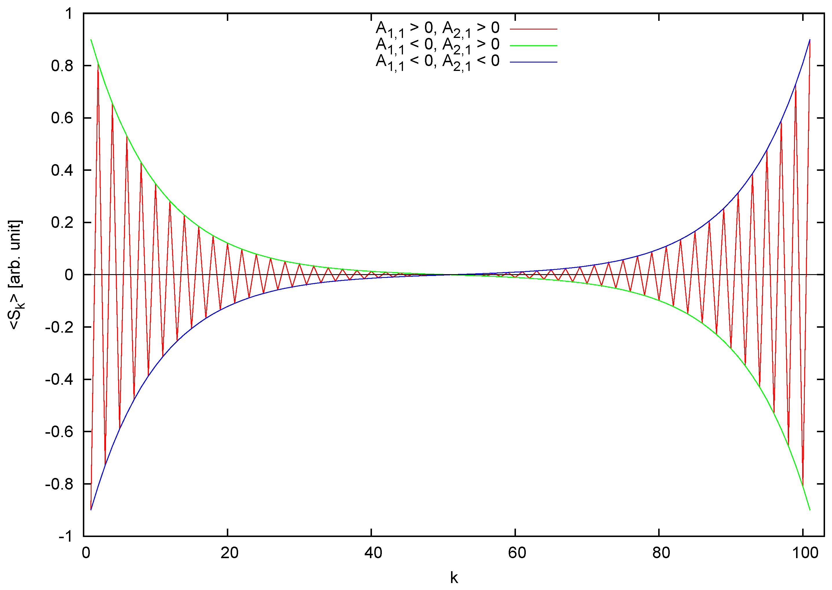
• $\langle S_k^{-}\rangle$ is an oscillating function of k, bounded by the two sequences $S_k^{+}$ with opposite values of $A_{2,1}$ (also seen in Monte Carlo simulations).
• The sequence $\left\{S_k^{+}\right\}$ converges to 0 as $k\to \infty$ $\forall \rho :\left|\rho \right|<1$ and to 1 if $\rho =1$ (convergent sequence bounded theorem [4]). The existence of these limits makes a sound point for the consistency of the model in the thermodynamic limit (cf. Section 4).

The behavior of $\langle S_k\rangle$ is sketched in Figure 1.

2.3. Higher Order Expansion

The general treatment of Section 2 is valid at every order. It is easily seen that by replacing $A_{1,1}$ with $A^{\mathrm{u}}$, $A_{2,1}$ with $A^{\mathrm{gu}}$, and $A_{2,2}$ with $A^{\mathrm{g}}$ all the results obtained are still valid, for instance

$$\langle S_k\rangle =\frac{{\lambda }_1^{N+1}}{Z}({\rho }^k-{\rho }^{N-k+1})sinh(-2\beta A^{\mathrm{gu}}),$$

(44)

where

$$\rho =\frac{{\lambda }_2}{{\lambda }_1}=tanh(-\beta A^{\mathrm{u}}).$$

(45)

In the following, to keep the notation light, we keep considering the second order expansion.

3. Molecular Symmetry and Symmetry Breaking in the Hamiltonian

In Section 2, we have seen that, as long as the molecules on the chain have a non-zero odd-ranked multipole l together with a non-zero $l+1$ multipole, a bi-polar state may appear as a result of the broken spin flip symmetry of the Hamiltonian (6). This occurrence is of course closely connected with the molecule symmetry. We stress that no other assumption has been made on the molecules forming the system. The bi-polar state is, in that respect, a universal feature. From a standpoint of group symmetry, we notice that molecules with a center of inversion, i.e., of the $C_i$ point group, cannot have an l-ranked quadrupole with l odd and, therefore, no symmetry breaking can occur. On the contrary, $C_n$, $C_{n\nu }$, and $C_s$ have a non-zero dipole and quadrupole, and, therefore, the symmetry breaking occurs and a bi-polar state may show up.

In the next subsections, we will examine three more significant point groups and calculate the expectation value of the order parameter. The method outlined can, however, be employed for all point groups using the corresponding character tables [5,6]. Attention should be paid considering the appropriate orientation of the molecules in the chain to match the symmetry of the molecule.

We have already noticed that, roughly speaking, symmetry breaking cannot occur if the building blocks do not have an appropriate symmetry, such as $C_i$. On the other side, symmetries can greatly simplify calculation and allow major generalization.

3.1. Point Group $C_n$, $n>2$

The $C_n$ with $n>2$ turns out to be the simplest molecular symmetry required to break the symmetry in the Hamiltonian, in the sense that this point group ensures the presence of a dipole and a quadrupole, both of them having only one component.

Let us consider a frame of reference with the z-axis along the chain and assume also the molecule principal axis parallel to the z-axis. In this configuration, both the dipole and quadrupole have only the z-component non-zero, i.e., $q_1^0$,$q_2^0$ respectively. The relevant terms $A_{h,k}$ in Equations (17) and (19) for $C_n$, $n>2$ molecules are

$$\begin{array}{ccc}{A}_{1,1}\hfill & =& {\displaystyle -\sqrt{\frac{15}{2\pi }}{k}_C{\left(q_1^0\right)}^2<0},\hfill \\ \\ A_{2,1}\hfill & =& -A_{1,2}={\displaystyle -\frac{3}{2}\sqrt{\frac{7}{\pi }}{k}_C\frac{q_1^0{q}_2^0}{r^4}},\hfill \\ \\ A_{2,2}\hfill & =& {\displaystyle \frac{9}{\sqrt{(}\pi )}{k}_C\frac{{\left(q_2^0\right)}^2}{r^5}}.\hfill \end{array}$$

(46)

Since $A_{1,1}$ is negative, the order parameter should have the $S^{+}$ behavior.

3.2. Point Group $C_{2v}$

The symmetry of this point group requires $Q_1^{\pm 1}=0$ and $Q_2^{\pm 1}=0$, and, therefore, the matrices of interactions are given by

$$\begin{array}{ccc}{A}_{1,1}\hfill & =& -k_C{I}_2^0\left(z\right)\left(\begin{array}{ccc}0& q_1^0& 0\end{array}\right)\left(\begin{array}{ccc}0& 0& 1\\ 0& 2& 0\\ 1& 0& 0\end{array}\right)\left(\begin{array}{c}0\\ q_1^0\\ 0\end{array}\right)\hfill \\ \\ A_{2,1}\hfill & =& -\sqrt{3}{k}_C{I}_3^0\left(z\right)\left(\begin{array}{ccccc}{q}_2^0& 0& q_0^0& 0& q_0^{-2}\end{array}\right)\left(\begin{array}{ccc}0& 0& 0\\ 1& 0& 0\\ 0& \sqrt{3}& 0\\ 0& 0& 1\\ 0& 0& 0\end{array}\right)\left(\begin{array}{c}0\\ q_1^0\\ 0\end{array}\right)\hfill \\ \\ A_{1,2}\hfill & =& -A_{2,1}\hfill \\ \\ A_{2,2}\hfill & =& k_C{I}_4^0\left(z\right)\left(\begin{array}{ccccc}{q}_2^0& 0& q_0^0& 0& q_0^{-2}\end{array}\right)\left(\begin{array}{ccccc}0& 0& 0& 0& 1\\ 0& 0& 0& 2& 0\\ 0& 0& 6& 0& 0\\ 0& 2& 0& 0& 0\\ 1& 0& 0& 0& 0\end{array}\right)\left(\begin{array}{c}{q}_2^0\\ 0\\ q_0^0\\ 0\\ q_0^{-2}\end{array}\right)\hfill \end{array}.$$

(47)

Since $A_{1,1}$ is negative, the order parameter shows again the $S^{+}$ behavior.

3.3. Oscillating Behavior: The $C_{\mathrm{s}}$ Point Group

The general behavior of $\langle S_k\rangle$ is, at second order, eventually determined by the sign of $A_{1,1}$, specifically $A_{1,1}>0$ corresponds to an oscillating behavior. We shall look at this possibility more in detail. Since $I_2^0\left(\mathbf{r}\right)>\mathbf{0}$ $\forall \mathbf{r}$, the condition for oscillating behavior reads

$$\left(\begin{array}{ccc}{q}_1^1& q_1^0& -{q_1^1}^{*}\end{array}\right)\left(\begin{array}{ccc}0& 0& 1\\ 0& 2& 0\\ 1& 0& 0\end{array}\right)\left(\begin{array}{c}{q}_1^1\\ q_1^0\\ -{q_1^1}^{*}\end{array}\right)=2({\left(q_1^0\right)}^2-|q_1^1{|}^2)<0,$$

(48)

where ${}^{*}$ denotes complex conjugate and we have used the relation $q_l^{-m}={(-1)}^l{\left(q_l^m\right)}^{*}$. Thus, the $S^{-}$ behavior should be expected when

$$|q_1^1|-|q_1^0|>0.$$

(49)

This inequality is surely verified if $q_1^0=0$.

Let us consider a chain of molecules with $C_{\mathrm{s}}$ symmetry, oriented with the mirror plane orthogonal to the chain direction. The z-axis is assumed, as usual, parallel to the chain. In this case, $q_1^0=0$ and the oscillation behavior should be expected.

4. Macroscopic Systems

A d-dimensional Ising lattice model is defined on a finite subset ${\Gamma }_L$ of integers $Z^d$, the number of spin variable configurations ${\left\{S_i\right\}}_{i\in \Gamma }$ is therefore finite. In order to extrapolate results for macroscopic system, we consider the limit of ${\Gamma }_L$ with free boundary condition for $L\to \infty$. Note that averaged quantities depend in general on the nature of the boundary conditions. We demonstrate that in the canonical ensemble, the thermodynamic limit of the free energy per site exists and is finite for the model considered. The free energy is given by $F=-k_{B}TlnZ$. Using Equation (34), the free energy per site at the second order can be expressed in the limit of large systems as

$$f\left(T\right)=\frac{F}{N}=-\frac{1}{\beta N}ln\{{\lambda }_1^N[1+cosh\left(2\beta A_{2,1}\right]\}=-\frac{ln{\lambda }_1}{\beta }-\frac{lncosh\left(2\beta A_{2,1}\right)}{\beta N}for N\gg 1.$$

(50)

At every finite temperature, therefore, the limit

$$\underset{N\to \infty }{lim}\frac{F}{N}=-\frac{lncosh\left(\beta A_{1,1}\right)}{\beta }$$

(51)

exists and is finite. Analogously, the averaged energy of the system $\langle E\rangle$, which is the thermodynamical internal energy U, is given by

$$U=\langle E\rangle =-\frac{\partial }{\partial \beta }lnZ=N{A}_{1,1}tanh\left(\beta A_{1,1}\right)for N\gg 1.$$

(52)

Note the explicit appearance of the extensivity in the energy due to the factor N. The energy fluctuations are given by

$$\langle {(\Delta E)}^2\rangle =-\frac{\partial \langle E\rangle }{\partial \beta }=T^2{k}_B\frac{\partial \langle E\rangle }{\partial T}=A_{1,1}^{2}N[{tanh}^2\left(\beta A_{1,1}\right)-1]for N\gg 1.$$

(53)

The specific heat is given by

$$c_v=\frac{\partial \langle E\rangle }{\partial T}=\frac{\langle {(\Delta E)}^2\rangle }{k_B{T}^2}=N\frac{{\left(\beta A_{1,1}\right)}^2[1-{tanh}^2\left(\beta A_{1,1}\right)]}{k_B}.$$

(54)

We notice that the non-diagonals terms of the coupling parameters $A_{i,j}$, $i\ne j$, which are essential for the symmetry breaking in the Hamiltonian and, ultimately, to the onset of spontaneous polarization do not enter the fundamental extensive thermodynamic quantities.

We conclude this section by showing that the free energy per site is a concave function of the absolute temperature. This is easily accomplished by observing that, since $f\in C^2\left(\mathcal{R}\right)$

$$\frac{{\partial }^{2}f}{\partial T^2}=-\frac{A_{1,1}^2}{k_B{T}^3}{\text{sech}}^2\left(\beta A_{1,1}\right)<0\forall T,\forall A_{1,1}.$$

(55)

In consideration that the thermodynamic properties at equilibrium are determined by the free energy, this last statement ensures the thermodynamic stability of the model [7].

5. Conclusions

Starting from a generalized Ising model with the electrostatic interactions given in multipole expansion, we have shown that the onset of polarity in a molecular system can be described as the result of two symmetry breaking effects: the translational and the global spin flip invariance. The former is of geometrical origin and is reflected by the presence of free boundary conditions, the latter is explained as the effect of specific multipole interactions. The spontaneous polarization is assessed by the thermal average of the order parameter $\langle S\rangle$ analogous to the average magnetization of the standard Ising model. The analysis of $\langle S\rangle$ as a function of the length inside the system shows two different behaviors depending on the sign of the asymmetric interaction of same odd order multipoles (e.g., dipole-dipole): an S-shaped odd function characteristic of spin correlations fading out inside the system, and an oscillating function corresponding to an alternate ordering of plus/minus spins.

The thermodynamic limit is shown to exist under very general conditions, and the concavity of the free energy per lattice site demonstrates the thermodynamic stability of the model. At a second order treatment, the asymmetric interactions (e.g., the dipole-quadrupole one), which are crucial for the Hamiltonian symmetry breaking, do not enter any of the macroscopic thermodynamic quantities such as the free energy and specific heat. These latter quantities appear to be only determined by the symmetric (e.g., dipole-dipole) interactions. Asymmetric interactions seem, therefore, to only trigger the onset of polarity by a symmetry breaking process, leaving other thermodynamic properties, including the general behavior of $\langle S\rangle$, unaffected.

The extension of the previous analysis to higher spatial dimensions and to off-lattice models is a priority for us, and, to this goal, works are already on the way. Along with theoretical calculations, large scale Monte Carlo and molecular dynamics simulations with more complex force fields are running and will be the object of forthcoming publications.

References

- Hulliger, J.; Wüst, T.; Brahimi, K.; Martinez Garcia, J.C. Can Mono Domain Polar Molecular Crystals Exist? Cryst. Growth Des. 2012, 12, 5211–5218. [Google Scholar] [CrossRef]
- Bebie, H.; Hulliger, J. Thermal equilibrium polarization: A near-surface effect in dipolar-based molecular crystals. Phys. A: Stat. Mech. Its Appl. 2000, 278, 327–336. [Google Scholar] [CrossRef]
- Baxter, R.J. Exactly Solved Models in Statistical Mechanics; Academic Press: New York, NY, USA, 1982; p. 89. [Google Scholar]
- Courant, R. Differential and Integral Calculus; Blackie & Son: Glasgow, UK, 1961; Volume I, p. 40. [Google Scholar]
- Stone, A. The Theory of Intermolecular Forces, 2nd ed.; Oxford University Press: New York, NY, USA, 2013; p. 34. [Google Scholar]
- Gelessus, A.; Thiel, W.; Weber, W. Multipoles and Symmetry. J. Chem. Educ. 1995, 72, 505. [Google Scholar] [CrossRef]
- Lieb, E.H. The Stability of Matter: From Atoms to Stars; Springer: Berlin, Germany, 2013; p. 567. [Google Scholar]
Figure 1.
General behavior of the average order parameter vs. distance on the chain. For clarity, the curve corresponding to and has been omitted as it is simply the oscillating curve plotted with reversed sign. The values have been arbitrarily chosen.
© 2016 by the authors; licensee MDPI, Basel, Switzerland. This article is an open access article distributed under the terms and conditions of the Creative Commons by Attribution (CC-BY) license (http://creativecommons.org/licenses/by/4.0/).
Share and Cite
MDPI and ACS Style
Cannavacciuolo, L.; Hulliger, J. Polarity Formation in Molecular Crystals as a Symmetry Breaking Effect. Symmetry 2016, 8, 10. https://doi.org/10.3390/sym8030010
AMA Style
Cannavacciuolo L, Hulliger J. Polarity Formation in Molecular Crystals as a Symmetry Breaking Effect. Symmetry. 2016; 8(3):10. https://doi.org/10.3390/sym8030010
Chicago/Turabian StyleCannavacciuolo, Luigi, and Jürg Hulliger. 2016. "Polarity Formation in Molecular Crystals as a Symmetry Breaking Effect" Symmetry 8, no. 3: 10. https://doi.org/10.3390/sym8030010
Note that from the first issue of 2016, this journal uses article numbers instead of page numbers. See further details here.