
A Novel Texture Feature Description Method Based on the Generalized Gabor Direction Pattern and Weighted Discrepancy Measurement Model

Abstract
:1. Introduction
- (1)
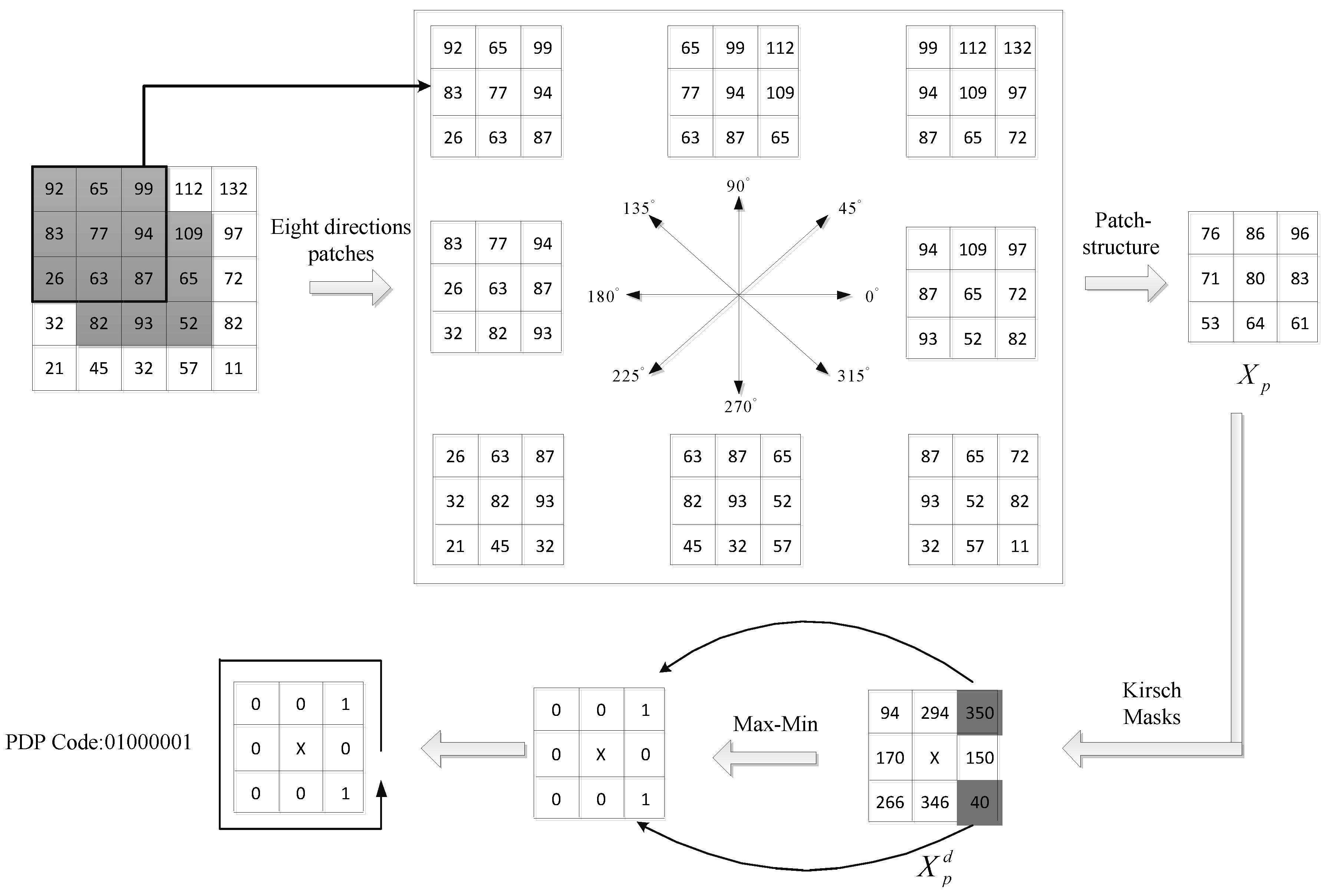
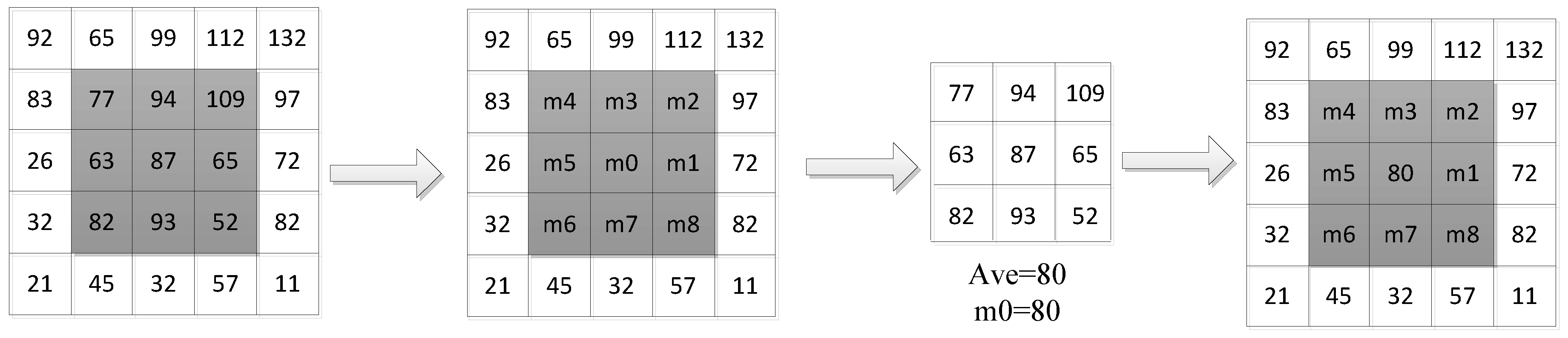
- Conventional LBP computes the relationship between one image’s center pixel value and its neighbor pixel value, and always only utilizes the center pixel’s direction information. LBP cannot obtain more detailed direction information from other neighborhood pixels, and thus is sensitive to noise. To overcome these defects, we propose a novel patch-structure direction pattern (PDP) method, which can extract richer feature information and be insensitive to noise.
- (2)
- To further improve the effectiveness of PDP, we introduce it into multi-channel Gabor space and get an improved method called GGDP, which can better describe multi-direction and multi-scale texture information.
- (3)
- In the traditional classification process, the GGDP feature of each Gabor sub-image should be concatenated and measured. To make the measurement of feature distance more accurate, WDMM is proposed for measuring every GGDP feature of the Gabor sub-image distance and use weighted computing for the final distance with sub-image information content.
2. Algorithm Description
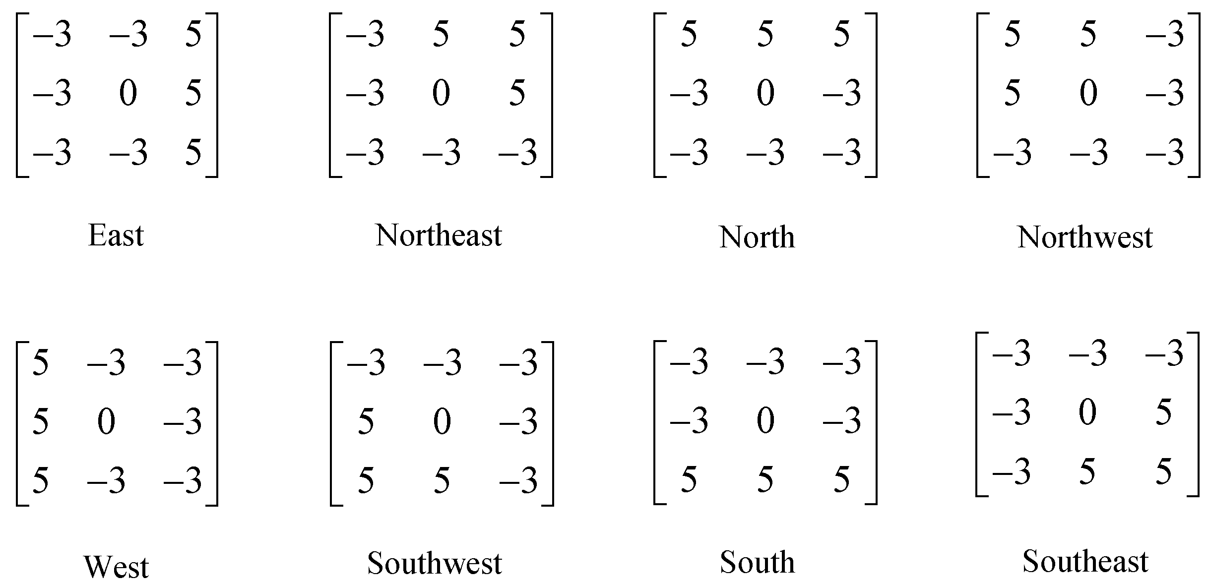
2.1. PDP
2.2. GGDP
2.3. WDMM
3. Experiments
3.1. Performance of the Proposed Method
3.1.1. Discussion of Computational Time
3.1.2. Discussion on Classification
3.2. Experiments and Analysis on CMUPIE Database
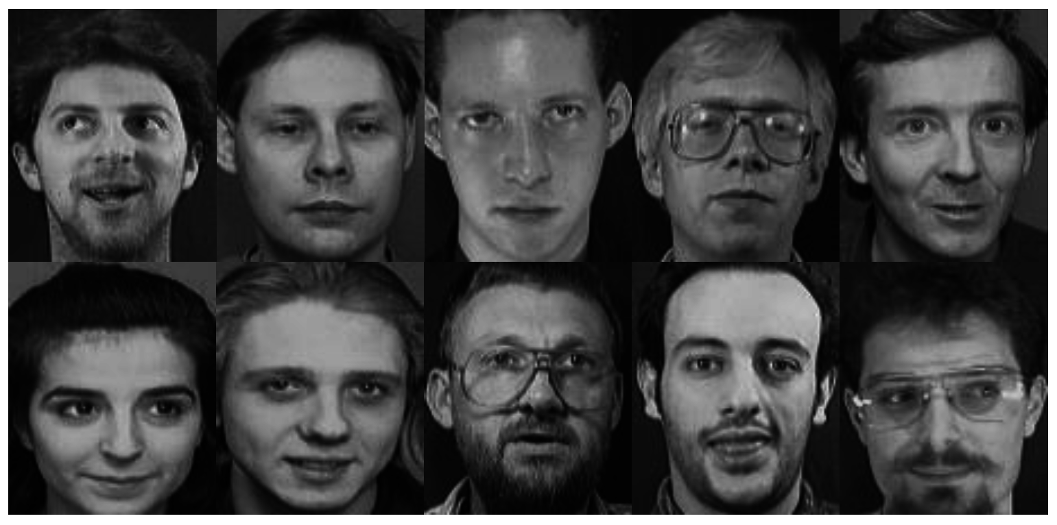
3.3. Experiments and Analysis on the ORL Database
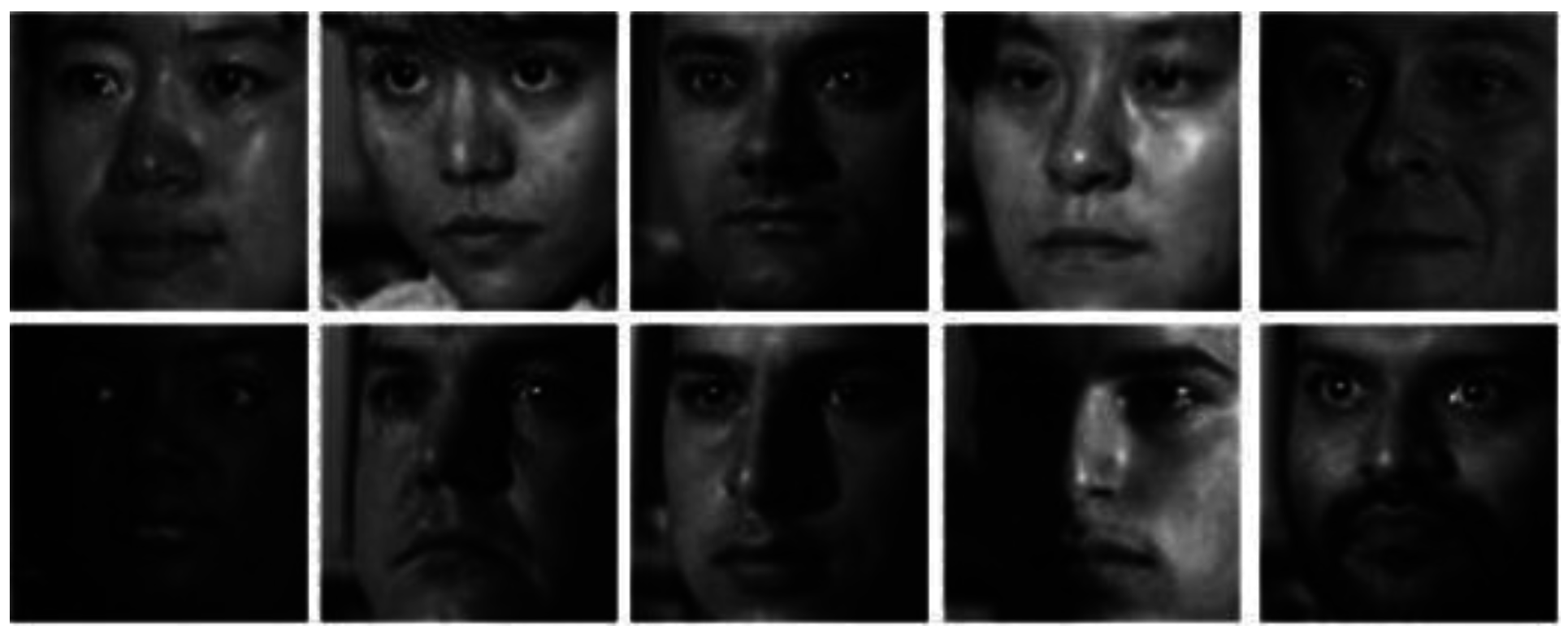
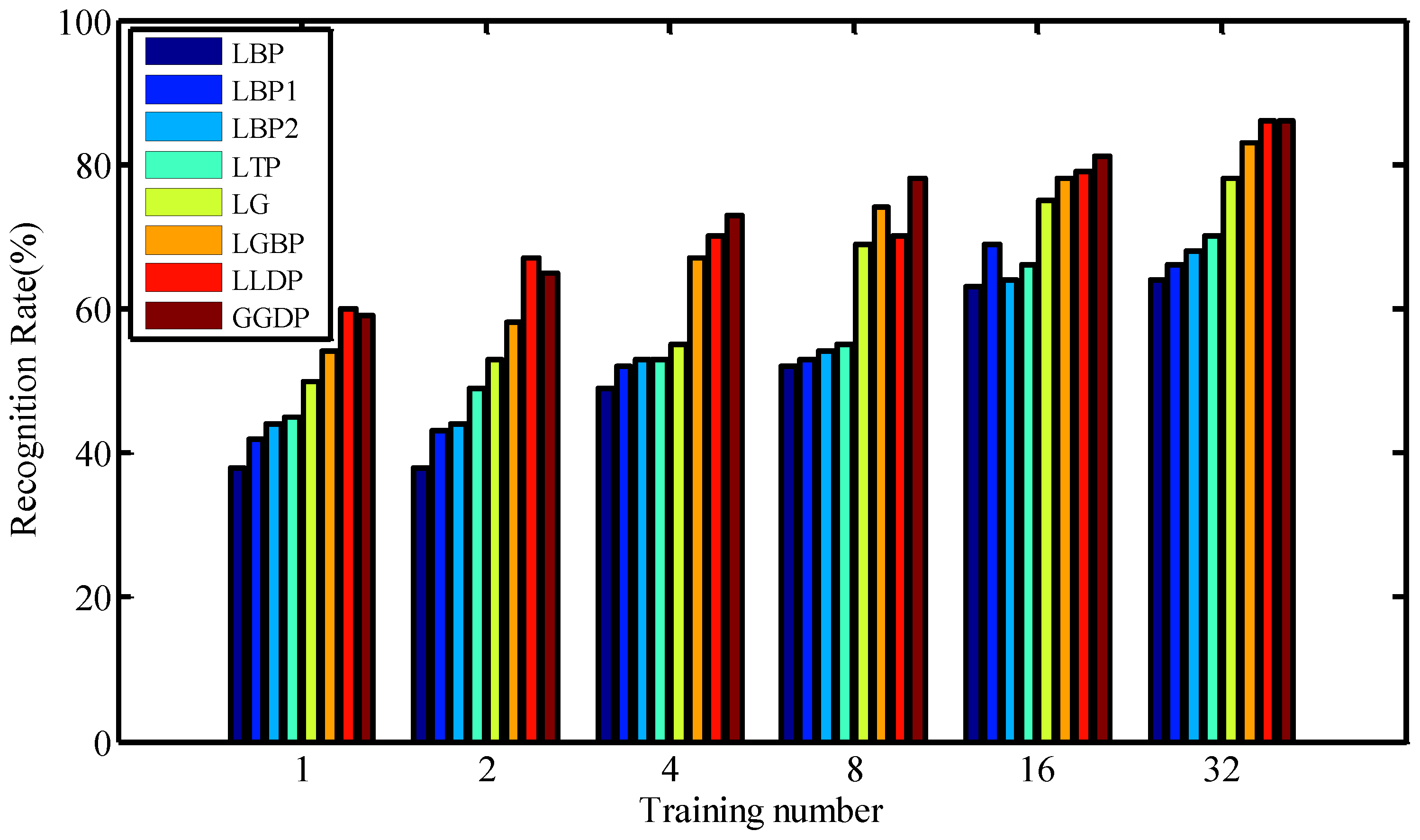
3.4. Experiments and Analysis on YALE B Database
4. Conclusions
Acknowledgments
Author Contributions
Conflicts of Interest
References
- Turk, M.A.; Pentland, A.P. Face recognition using eigenfaces. In Proceedings of the IEEE Computer Society Conference on Computer Vision and Pattern Recognition, Maui, HI, USA, 3–6 June 1991; IEEE: New York, NY, USA, 1991; pp. 586–591. [Google Scholar]
- Yang, J.; Liu, C. Horizontal and vertical 2DPCA-based discriminant analysis for face verification on a large-scale database. IEEE Trans. Inf. Forensics Secur. 2007, 2, 781–792. [Google Scholar] [CrossRef]
- Meng, J.; Zhang, W. Volume measure in 2DPCA-based face recognition. Pattern Recognit. Lett. 2007, 28, 1203–1208. [Google Scholar] [CrossRef]
- Huang, D.; Yi, Z.; Pu, X. A new incremental PCA algorithm with application to visual learning and recognition. Neural Process. Lett. 2009, 30, 171–185. [Google Scholar] [CrossRef]
- Tan, K.; Chen, S. Adaptively weighted sub-pattern PCA for face recognition. Neurocomputing 2005, 64, 505–511. [Google Scholar] [CrossRef]
- Hsieh, P.C.; Tung, P.C. A novel hybrid approach based on sub-pattern technique and whitened PCA for face recognition. Pattern Recognit. 2009, 42, 978–984. [Google Scholar] [CrossRef]
- Belhumeur, P.N.; Hespanha, J.P.; Kriegman, D.J. Eigenfaces vs. fisherfaces: Recognition using class specific linear projection. IEEE Trans. Pattern Anal. Mach. Intell. 1997, 19, 711–720. [Google Scholar] [CrossRef]
- Fàbregas, J.; Faundez-Zanuy, M. Biometric dispersion matcher versus LDA. Pattern Recognit. 2009, 42, 1816–1823. [Google Scholar] [CrossRef]
- Strecha, C.; Bronstein, A.M.; Bronstein, M.M.; Fua, P. LDAHash: Improved matching with smaller descriptors. IEEE Trans. Pattern Anal. Mach. Intell. 2012, 34, 66–78. [Google Scholar] [CrossRef] [PubMed]
- Oh, J.H.; Kwak, N. Generalization of linear discriminant analysis using Lp-norm. Pattern Recognit. Lett. 2013, 34, 679–685. [Google Scholar] [CrossRef]
- Zhao, C.; Miao, D.; Lai, Z.; Gao, C.; Liu, C.; Yang, J. Two-dimensional color uncorrelated discriminant analysis for face recognition. Neurocomputing 2013, 113, 251–261. [Google Scholar] [CrossRef]
- Selvan, S.; Borckmans, P.B.; Chattopadhyay, A.; Absil, P.-A. Spherical mesh adaptive direct search for separating quasi-uncorrelated sources by range-based independent component analysis. Neural Comput. 2013, 25, 2486–2522. [Google Scholar] [CrossRef] [PubMed]
- Sun, Z.L.; Lam, K.M. Depth estimation of face images based on the constrained ICA model. IEEE Trans. Inf. Forensics Secur. 2011, 6, 360–370. [Google Scholar] [CrossRef]
- Fernandes, S.L.; Bala, G.J. A comparative study on ICA and LPP based Face Recognition under varying illuminations and facial expressions. In Proceedings of the 2013 International Conference on Signal Processing Image Processing & Pattern Recognition, Coimbatore, India, 7–8 February 2013; IEEE: New York, NY, USA, 2013; pp. 122–126. [Google Scholar]
- Wu, M.; Zhou, J.; Sun, J. Multi-scale ICA texture pattern for gender recognition. Electron. Lett. 2012, 48, 629–631. [Google Scholar] [CrossRef]
- Li, S.; Lu, H.C.; Ruan, X.; Chen, Y.-W. Human body segmentation based on independent component analysis with reference at two-scale superpixel. IET Image Process. 2012, 6, 770–777. [Google Scholar] [CrossRef]
- Shin, K.; Feraday, S.A.; Harris, C.J.; Brennan, M.J.; Oh, J.-E. Optimal autoregressive modeling of a measured noisy deterministic signal using singular-value decomposition. Mech. Syst. Signal Process. 2003, 17, 423–432. [Google Scholar] [CrossRef]
- Wei, J.J.; Chang, C.J.; Chou, N.K.; Jan, G.J. ECG data compression using truncated singular value decomposition. IEEE Trans. Inf. Technol. Biomed. 2001, 5, 290–299. [Google Scholar] [PubMed]
- Walton, J.; Fairley, N. Noise reduction in X-ray photoelectron spectromicroscopy by a singular value decomposition sorting procedure. J. Electron Spectrosc. Relat. Phenom. 2005, 148, 29–40. [Google Scholar] [CrossRef]
- Do, M.N.; Vetterli, M. Wavelet-based texture retrieval using generalized Gaussian density and Kullback-Leibler distance. IEEE Trans. Image Process. 2002, 11, 146–158. [Google Scholar] [CrossRef] [PubMed]
- Ahmadian, A.; Mostafa, A. An efficient texture classification algorithm using Gabor wavelet. In Proceedings of the 25th Annual International Conference of the IEEE Engineering in Medicine and Biology Society, Cancun, Mexico, 17–21 September 2003; IEEE: New York, NY, USA, 2003; Volume 1, pp. 930–933. [Google Scholar]
- Ye, F.; Shi, Z.; Shi, Z. A comparative study of PCA, LDA and Kernel LDA for image classification. In Proceedings of the International Symposium on Ubiquitous Virtual Reality, Gwangju, Korea, 8–11 July 2009; IEEE: New York, NY, USA, 2009; pp. 51–54. [Google Scholar]
- Ojala, T.; Pietikäinen, M.; Mäenpää, T. A generalized Local Binary Pattern operator for multiresolution gray scale and rotation invariant texture classification. In Proceedings of the International Conference on Advances in Pattern Recognition, Rio de Janeiro, Brazil, 11–14 March 2001; Volume 1, pp. 397–406.
- Ojala, T.; Pietikäinen, M.; Mäenpää, T. Multiresolution gray-scale and rotation invariant texture classification with local binary patterns. IEEE Trans. Pattern Anal. Mach. Intell. 2002, 24, 971–987. [Google Scholar] [CrossRef]
- Tan, X.; Triggs, B. Enhanced local texture feature sets for face recognition under difficult lighting conditions. IEEE Trans. Image Process. 2010, 19, 1635–1650. [Google Scholar] [PubMed]
- Zhou, S.R.; Yin, J.P.; Zhang, J.M. Local binary pattern (LBP) and local phase quantization (LBQ) based on Gabor filter for face representation. Neurocomputing 2013, 116, 260–264. [Google Scholar] [CrossRef]
- Zhang, B.; Gao, Y.; Zhao, S.; Liu, J. Local derivative pattern versus local binary pattern: Face recognition with high-order local pattern descriptor. IEEE Trans. Image Process. 2010, 19, 533–544. [Google Scholar] [CrossRef] [PubMed]
- Yang, X.; Cheng, K.T. Local difference binary for ultrafast and distinctive feature description. IEEE Trans. Pattern Anal. Mach. Intell. 2014, 36, 188–194. [Google Scholar] [CrossRef] [PubMed]
- Luo, Y.T.; Zhao, L.Y.; Zhang, B.; Jia, W.; Xue, F.; Lu, J.-T.; Zhu, Y.-H.; Xu, B.-Q. Local line directional pattern for palmprint recognition. Pattern Recognit. 2016, 50, 26–44. [Google Scholar] [CrossRef]
- Qian, X.; Hua, X.S.; Chen, P.; Ke, L. PLBP: An effective local binary patterns texture descriptor with pyramid representation. Pattern Recognit. 2011, 44, 2502–2515. [Google Scholar] [CrossRef]
- Murala, S.; Maheshwari, R.P.; Balasubramanian, R. Local tetra patterns: A new feature descriptor for content-based image retrieval. IEEE Trans. Image Process. 2012, 21, 2874–2886. [Google Scholar] [CrossRef] [PubMed]
- Liao, S.; Law, M.W.K.; Chung, A. Dominant local binary patterns for texture classification. IEEE Trans. Image Process. 2009, 18, 1107–1118. [Google Scholar] [CrossRef] [PubMed]
- Calonder, M.; Lepetit, V.; Strecha, C.; Fua, P. Brief: Binary robust independent elementary features. In Proceedings of the European Conference on Computer Vision-ECCV, Heraklion, Greece, 5–11 September 2010; pp. 778–792.
- Verma, M.; Raman, B. Local tri-directional patterns: A new texture feature descriptor for image retrieval. Digit. Signal Process. 2016, 51, 62–72. [Google Scholar] [CrossRef]
- Chen, X.; Zhou, Z.; Zhang, J.; Liu, Z.; Huang, Q. Local convex-and-concave pattern: An effective texture descriptor. Inf. Sci. 2016, 363, 120–139. [Google Scholar] [CrossRef]
- Zhang, H.; He, P.; Yang, X. Fault detection based on multi-scale local binary patterns operator and improved teaching-learning-based optimization algorithm. Symmetry 2015, 7, 1734–1750. [Google Scholar] [CrossRef]
- Mukundan, R. Local Tchebichef Moments for Texture Analysis; Moments and Moment Invariants—Theory and Applications; Science Gate Publishing: Thrace, Greece, 2014; Volume 1, pp. 127–142. [Google Scholar]
- Papakostas, G.A.; Koulouriotis, D.E.; Karakasis, E.G.; Tourassis, V.D. Moment-based local binary patterns: A novel descriptor for invariant pattern recognition applications. Neurocomputing 2013, 99, 358–371. [Google Scholar] [CrossRef]
- Nanni, L.; Brahnam, S.; Ghidoni, S.; Emanuele, M.; Tonya, B. Different approaches for extracting information from the co-occurrence matrix. PLoS ONE 2013, 8, e83554. [Google Scholar] [CrossRef] [PubMed]
- Nanni, L.; Brahnam, S.; Ghidoni, S.; Menegatti, E. Region based approaches and descriptors extracted from the cooccurrence matrix. Int. J. Latest Res. Sci. Technol. 2014, 3, 192–200. [Google Scholar]
- Kanan, H.R.; Faez, K. Recognizing faces using Adaptively Weighted Sub-Gabor Array from a single sample image per enrolled subject. Image Vis. Comput. 2010, 28, 438–448. [Google Scholar] [CrossRef]
- Cament, L.A.; Castillo, L.E.; Perez, J.P.; Galdames, F.J.; Perez, C.A. Fusion of local normalization and Gabor entropy weighted features for face identification. Pattern Recognit. 2014, 47, 568–577. [Google Scholar] [CrossRef]
- Gao, T.; He, M. A novel face description by local multi-channel Gabor histogram sequence binary pattern. In Proceedings of the International Conference on Audio, Language and Image Processing, Shanghai, China, 7–9 July 2008; IEEE: New York, NY, USA, 2008; pp. 1240–1244. [Google Scholar]
- Xie, S.; Shan, S.; Chen, X.; Chen, J. Fusing local patterns of Gabor magnitude and phase for face recognition. IEEE Trans. Image Process. 2010, 19, 1349–1361. [Google Scholar] [PubMed]
- Sharma, P.; Arya, K.V.; Yadav, R.N. Efficient face recognition using wavelet-based generalized neural network. Signal Process. 2013, 93, 1557–1565. [Google Scholar] [CrossRef]
- Zuñiga, A.G.; Florindo, J.B.; Bruno, O.M. Gabor wavelets combined with volumetric fractal dimension applied to texture analysis. Pattern Recognit. Lett. 2014, 36, 135–143. [Google Scholar] [CrossRef]
- Găianu, M.; Onchiş, D.M. Face and marker detection using Gabor frames on GPUs. Signal Process. 2014, 96, 90–93. [Google Scholar] [CrossRef]
- Zhao, Z.S.; Zhang, L.; Zhao, M.; Hou, Z.-G.; Zhang, C.-S. Gabor face recognition by multi-channel classifier fusion of supervised kernel manifold learning. Neurocomputing 2012, 97, 398–404. [Google Scholar] [CrossRef]


| Method Abbreviation | Method Explanation |
|---|---|
| LBP [23] | Basic LBP features |
| LBP1 [24] | LBP (8, 1) features |
| LBP2 [24] | LBP (8, 2) features |
| LTP [25] | LTP features |
| LG [40] | Local Gabor |
| LGBP [42] | Local Gabor Binary Pattern |
| LLDP [29] | Local Line Directional Pattern |
| GGDP | Generalized Gabor Direction Patterns |
| Descriptor | Feature Dimension | Feature Extract Times (ms) |
|---|---|---|
| LBP [1] | 256 | 97.4 |
| LG [40] | 393,216 | 294.2 |
| LGBP [42] | 6144 | 326.4 |
| GGDP | 6144 | 386.5 |
| Recognition Methods | Training Sample Numbers | |||||
|---|---|---|---|---|---|---|
| 1 | 2 | 4 | 6 | 8 | 10 | |
| GGDP + NN | 44.71% | 56.08% | 62.65% | 67.94% | 73.14% | 81.08% |
| GGDP + SVM | 45.98% | 76.76% | 81.76% | 87.35% | 88.33% | 91.08% |
| GGDP + WDMM | 56.76% | 75.39% | 83.73% | 86.18% | 90.98% | 93.82% |
| Recognition Methods | Training Sample Numbers | |||||
|---|---|---|---|---|---|---|
| 1 | 2 | 4 | 6 | 8 | 10 | |
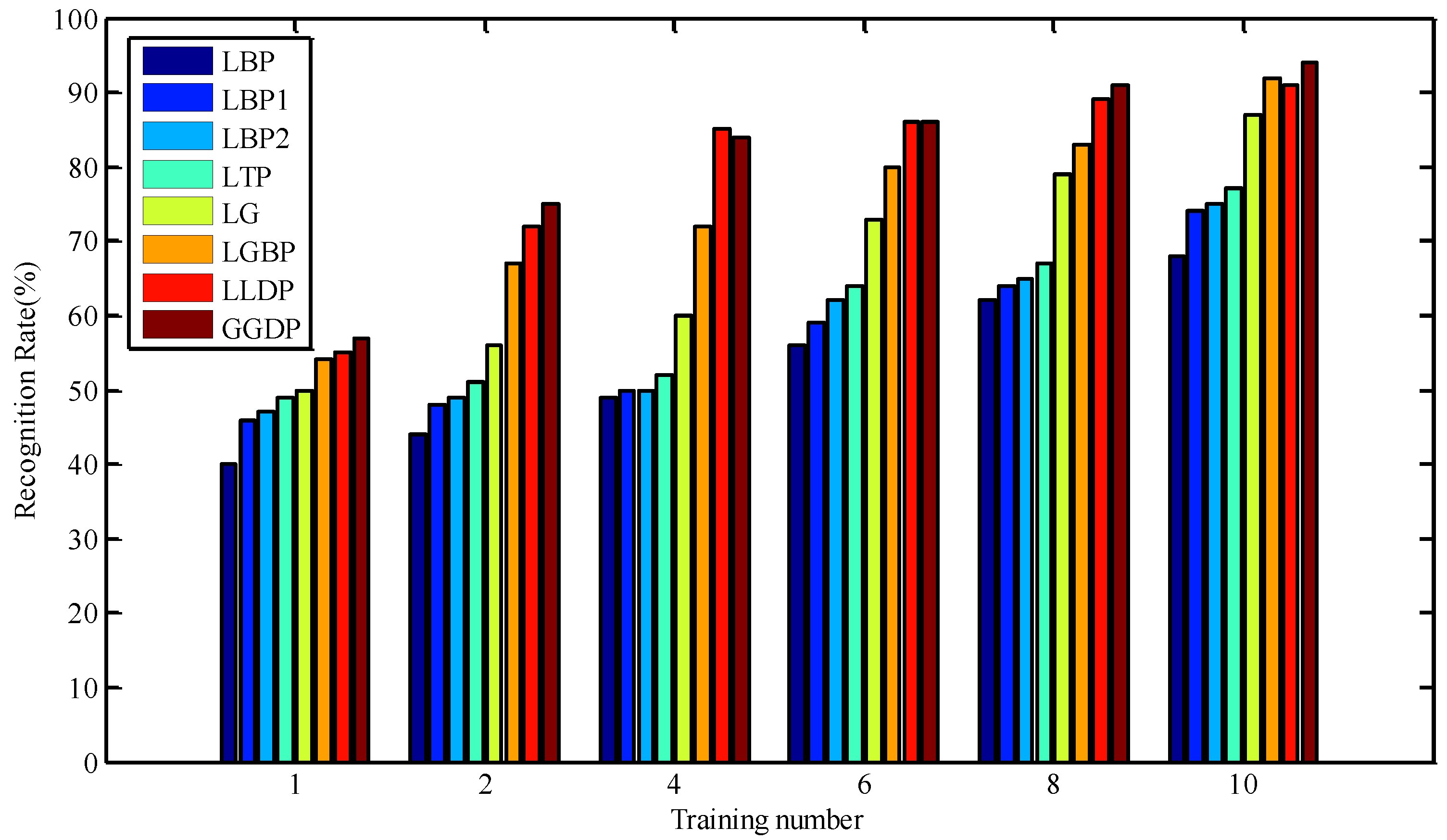
| LBP | 40.29% | 44.41% | 48.92% | 55.98% | 62.45% | 68.14% |
| LBP1 | 46.18% | 47.84% | 49.71% | 58.73% | 64.02% | 73.92% |
| LBP2 | 47.35% | 48.92% | 50.20% | 61.57% | 65.10% | 75.10% |
| LTP | 49.31% | 50.59% | 51.76% | 63.53% | 66.86% | 76.67% |
| LG | 50.20% | 55.59% | 60.10% | 73.14% | 79.12% | 87.45% |
| LGBP | 54.02% | 67.35% | 72.06% | 80.29% | 83.43% | 91.86% |
| LLDP | 55.49% | 72.45% | 85.20% | 85.78% | 89.31% | 91.27% |
| GGDP | 56.76% | 75.39% | 83.73% | 86.18% | 90.98% | 93.82% |
| Recognition Methods | Training Sample Numbers | |||||
|---|---|---|---|---|---|---|
| 1 | 2 | 3 | 4 | 5 | 6 | |
| LBP | 53.75% | 55.50% | 64.00% | 76.50% | 83.75% | 84.25% |
| LBP1 | 55.75% | 56.00% | 65.50% | 81.00% | 85.25% | 85.50% |
| LBP2 | 58.50% | 59.00% | 65.25% | 81.50% | 88.00% | 88.50% |
| LTP | 60.25% | 61.50% | 69.00% | 83.50% | 87.25% | 88.25% |
| LG | 64.25% | 69.75% | 72.25% | 83.00% | 88.00% | 91.50% |
| LGBP | 65.75% | 70.75% | 75.50% | 87.00% | 90.75% | 95.25% |
| LLDP | 63.25% | 72.25% | 75.75% | 86.50% | 92.25% | 96.50% |
| GGDP | 70.25% | 74.75% | 78.00% | 90.25% | 93.25% | 98.00% |
| Recognition Methods | Training Sample Numbers | |||||
|---|---|---|---|---|---|---|
| 1 | 2 | 4 | 8 | 16 | 32 | |
| LBP | 37.91% | 38.22% | 48.94% | 51.72% | 63.19% | 63.53% |
| LBP1 | 42.31% | 42.69% | 52.44% | 53.09% | 69.25% | 66.06% |
| LBP2 | 43.63% | 44.44% | 52.78% | 53.84% | 64.25% | 67.91% |
| LTP | 44.53% | 48.84% | 53.22% | 55.09% | 65.72% | 69.88% |
| LG | 49.59% | 53.01% | 55.48% | 68.77% | 75.21% | 78.36% |
| LGBP | 53.56% | 58.36% | 66.99% | 73.56% | 77.95% | 82.60% |
| LLDP | 59.72% | 66.59% | 69.66% | 70.34% | 79.34% | 85.78% |
| GGDP | 58.63% | 64.52% | 72.60% | 78.22% | 81.37% | 86.44% |
© 2016 by the authors; licensee MDPI, Basel, Switzerland. This article is an open access article distributed under the terms and conditions of the Creative Commons Attribution (CC-BY) license (http://creativecommons.org/licenses/by/4.0/).
Share and Cite
Chen, T.; Zhao, X.; Dai, L.; Zhang, L.; Wang, J. A Novel Texture Feature Description Method Based on the Generalized Gabor Direction Pattern and Weighted Discrepancy Measurement Model. Symmetry 2016, 8, 109. https://doi.org/10.3390/sym8110109
Chen T, Zhao X, Dai L, Zhang L, Wang J. A Novel Texture Feature Description Method Based on the Generalized Gabor Direction Pattern and Weighted Discrepancy Measurement Model. Symmetry. 2016; 8(11):109. https://doi.org/10.3390/sym8110109
Chicago/Turabian StyleChen, Ting, Xiangmo Zhao, Liang Dai, Licheng Zhang, and Jiarui Wang. 2016. "A Novel Texture Feature Description Method Based on the Generalized Gabor Direction Pattern and Weighted Discrepancy Measurement Model" Symmetry 8, no. 11: 109. https://doi.org/10.3390/sym8110109