Computing with Colored Tangles

Abstract

We suggest a diagrammatic model of computation based on an axiom of distributivity. A diagram of a decorated colored tangle, similar to those that appear in low dimensional topology, plays the role of a circuit diagram. Equivalent diagrams represent bisimilar computations. We prove that our model of computation is Turing complete and with bounded resources that it can decide any language in complexity class IP, sometimes with better performance parameters than corresponding classical protocols.

1. Introduction

The present research represents a step in a program whose goal is to study topological aspects of information and computation. Time is a metric notion, and so, any such topological aspects would presumably have no internal notion of time. The present paper formulates a notion of computation that is independent of time and that is natively formulated in terms of information. We formulate a diagrammatic calculus whose elements we call tangle machines. These were first defined in [1]. A key feature of tangle machines is that they come equipped with a natural notion of equivalence, which originates in the beautiful diagrammatic algebra of low dimensional topology. Tangle machines serve in this paper as abstract flowcharts of information in computation. The computational paradigm that we propose contains Turing machines and interactive proofs (thus, it does not “lose anything”), and it also contains additional models (e.g., Section 8.1).

The world we observe around us evolves along a time axis, so a tangle machine could not be used as a blueprint for a classical computer. Time is a more nebulous concept in the quantum realm, however, and it might be that tangle machine constructions are relevant for adiabatic quantum computations or in other quantum contexts. In particular, they naturally incorporate the axiom of uniform no-cloning (Remark 5). The main relevance of our work would probably be to isolate and access natively topological aspects of classical and quantum computation. We also speculate that tangle machine computations can emerge physically via dynamical processes on a tangle machine, given a set of input colors, and that perhaps something like this actually occurs in nature. After all, natural computers are not Turing machines.

How might tangle machines manifest themselves in nature? The authors make the following speculation. Evolutionary biology provides an analogue to tangle machines in the notions of phenotype versus genotype [2,3]. The external characteristics of an organism, such as its appearance, physiology, morphology, as well as its behaviors are collectively known as the phenotype. The genotype, on the other hand, refers to the inherent and immutable information encoded in the genome. Two phenotypes may look entirely different, but may nevertheless share the same genotype. Could information about an organism be encoded as a tangle machine, where equivalent machines represent different phenotypes that share the same genotype? Might the process of evolution of an organism be described by a series of basic transformations akin to the Reidemeister moves exerted by the environment on the organism, which change its phenotype while preserving its genotype, along with occasional “violent” local moves on a current configuration that change its genotype? Might tangle machines describe a way in which nature processes its information primitives, that is its organisms?

There are two obvious advantages to a topological model of computation. The first is that it is very flexible by construction. Bisimilar computations (Definition 10) are represented by topologically equivalent objects, which are related in a simple way (Section 10). The second, which we do not discuss in this paper, is that we have a notion of topological invariants, which are characteristic quantities that are intrinsic to a bisimilarity class of computations.

In the Introduction, we briefly introduce tangle machines in Section 1.1 after which we state our main results in Section 1.2 and give scientific context in Section 1.3.

1.1. What Is a Tangle Machine Computation?

A tangle machine is built up of registers, each of which may hold an element of a set Q. The set Q comes equipped with a set B of binary operations representing basic computations. For $▹\in B$, we read $x▹y$ as “the result of running the program $▹y$ on input data x”. An alternative evocative image is that $x▹y$ is a “fusion of information x with information y using algorithm ▹”. Our binary operations satisfy the following axioms, which equip $(Q,B)$ with what is called a quandle structure (see Section 3.2 for this and extensions):

• Idempotence: $x▹x=x$ for all $x\in Q$ and for all $▹\in B$. Thus, x cannot concoct any new information from itself.
• Reversibility: The map $▹y:Q\to Q$, which maps each color $x\in Q$ to a corresponding color $x▹y\in Q$, is a bijection for all $(y,▹)\in (Q,B)$. In particular, if $x▹y=z▹y$ for some $x,y,z\in Q$ and for some $▹\in B$, then $x=z$. Thus, the input x of a computation may uniquely be reconstructed from the output $x▹y$ together with the program $▹y$.
• Distributivity: For all $x,y,z\in Q$ and for all $▹,▸\in B$:

  $$(x▹y)▸z=(x▸z)▹(y▸z).$$

  (1)
  This is the main property. It says that carrying out a computation $▸ z$ on an output $x▹y$ gives the same result as carrying out that computation both on the input x and also on the state y and then combining these as $(x▸z)▹(y▸z)$. In the context of information, this is a no double counting property [4].

Later in this paper, in Remark 5, we show that uniform no-cloning and no-deleting, which are fundamental properties of quantum information, follow from reversibility and distributivity for an appropriate coloring by a generalization of a quandle called a quagma. This observation argues for reversibility and distributivity as being nature’s most fundamental information symmetries.

The basic unit of computation in a tangle machine is an interaction representing multiple inputs $x_1,\dots ,x_k$ independently fed into a program $▹y$, as depicted in Figure 1. These are concatenated (perhaps also with wyes) to form a tangle machine; see Section 3.

Figure 1. An interaction in a machine, where $z_i\stackrel{\mathrm{def}}{=}{x}_i▹y$ for $i=1,2,\dots ,k$.

Figure 1. An interaction in a machine, where $z_i\stackrel{\mathrm{def}}{=}{x}_i▹y$ for $i=1,2,\dots ,k$.

A tangle machine computation begins with an initialization of a specified set of input registers to chosen colors in Q. A disjoint set of output registers is chosen. If the colors of the input registers uniquely determine colors for the output registers, then the colors of the output registers are the result of the computation. Otherwise, the computation cannot take place. (See Definition 6 and Figure 2). This provides a model of computation.

Figure 2. A sample computation. Determining colors for input registers ${\mathrm{In}}_1$ and ${\mathrm{In}}_2$ uniquely and instantaneously determines the color for the output register Out.

Figure 2. A sample computation. Determining colors for input registers ${\mathrm{In}}_1$ and ${\mathrm{In}}_2$ uniquely and instantaneously determines the color for the output register Out.

Remark 1. More generally, we may allow the result of the computation to be the (possibly empty) set of all possible colors of output registers. This level of generality is not required in this paper.

A tangle machine computation has the following features:

• Whereas the alphabet of a classical Turing machine is discrete (usually just zero and one and maybe two), the alphabet Q of a tangle machine can be any set, discrete or not. Two values of Q may be chosen to represent zero and one, while the rest may represent something else, perhaps electric signals.
• Whereas a Turing machine computation is sequential with each step depending only on the state of the read/write head and on the scanned signal, a tangle machine computation is instantaneous and is dictated by an oracle. Time plays no role in a tangle machine computation.
• A tangle machine computation may or may not be deterministic (colors may represent random variables and not their realizations), and it may or may not be bounded (contain a bounded number of interactions). Quandles and tangle machines are flexible enough to admit several different interpretations. In this paper, we use tangle machines to realize both logic gates (deterministic, composing perhaps unbounded computations) and interactive proof computations (probabilistic, bounded size).
• A tangle machine is flexible. There is a natural and intuitive set of local moves relating bisimilar tangle machine computations (Section 10).
• A tangle machine representation is abstract. A tangle machine computation takes place on the level of information itself, with no reference to time. The axioms of a quandle have intrinsic interpretation in terms of the preservation and non-redundancy of information.

1.2. Results

The purpose of this note is to show the following theorems:

Theorem 1. Any binary Boolean function can be realized by a tangle machine computation.

This statement is not new: a previous such realization (not with tangle machines, but with colored braids) is recalled in Section 4.3.

By Turing completeness of the Boolean circuit model, we have the following:

Corollary 2. Tangle machines (with an unbounded number of interactions) are Turing complete.

In Section 5, we further prove the following.

Theorem 3. Any Turing machine can be simulated by a tangle machine. Such a tangle machine is colored by a quandle $(Q,B)$ whose set of binary operations B has cardinality $\mathcal{O}\left(n\right)$ where n is the number of states in the finite control of the underlying Turing machine.

Tangle machines, whose notion of computation is based on an oracle, which produces output colors from input colors, can, in fact, perform super-Turing computations. See Remark 4.

Colors of registers in tangle machines evolve at interactions. If we bound the number of interactions, tangle machine computations include computations in a complexity class, which we call TangIP, which includes inside it a class that we call BraidIP. Letting χ denote the number of interactions in the machine, letting δ denote a “noise parameter” and letting c and s denote completeness and soundness correspondingly (see Section 2.3), we have the following:

Theorem 4. $\mathrm{IP}\subseteq \mathrm{BraidIP}\left\{\delta ,\chi \right\}$ where:

$$I\left(c\delta \right)<\chi <\frac{1}{I(1-s\delta )},$$

(2)

with $I\left(p\right)\stackrel{\mathrm{def}}{=}-p^{-1}logp$. The growth rate of χ is $\mathcal{O}\left(\frac{1}{\delta }\right)$ as $\delta \to 0$.

Thus, tangle machine computations with bounded interactions can decide any language in class IP, which is known to equal PSPACE [5].

Moreover, in the special setting of non-adaptive three-bit probabilistically-checkable proofs (PCP), there exists a tangle machine that achieves a better soundness parameter than the best known classical single-verifier non-adaptive three-bit PCP algorithm (Section 9.1). Yet, the soundness parameter for this tangle machine is above the conjectured lower limit. This suggests the possibility that tangle machines behave like very good single verifiers.

Finally, in Section 10, we discuss the equivalence of machines. Machine equivalence formally parallels the equivalence of tangled objects in low dimensional topology, and it gives us a formalism with which to discuss bisimulation. After justifying the definition, we introduce a notion of zero knowledge for machines, in which the proof is kept secure from untrusted verifiers at intermediate nodes.

Tangle machines are thus revealed to be a flexible model for computation.

1.3. Other Low Dimensional Topological Approaches to Computation

The first person to consider distributivity as an axiom of primary importance and to suggest diagrammatic calculi for logic (and perhaps by extension to computation) was American philosopher Charles Saunders Peirce. The following Peirce quotation was pointed out by Elhamdadi [6]: “These are other cases of the distributive principle…These formulae, which have hitherto escaped notice, are not without interest.” [7]

The idea to use diagrammatic calculi from low-dimensional topology to model computation was pioneered by Louis Kauffman, who used knot and tangle diagrams to study automata [8], nonstandard set theory and lambda calculus [9,10]. There is also a diagrammatic π calculus formulation of virtual tangles [11]. The diagrammatic calculus of braids (braids are a special class of tangles) also underlies topological quantum computing; see e.g., [12,13]. Universal logic gates (Toffoli gates) have been realized using colored braids [14,15,16]. This has led to a proposal for circuit obfuscation, masking the true purpose of a circuit, using braid equivalence [17]. Buliga has suggested to represent computations using a calculus of colored tangles, which is different from ours [18]. In another direction, a different diagrammatic calculus, originating in higher category theory, has been used in the theory of quantum information; see e.g., [19,20,21].

In our approach, the tangle diagrams themselves are computers, representing a flowchart of information during a computation whose basic operations are distributive (compare [22]). This is not a diagrammatic lambda calculus or pi calculus, but rather it is a natively low dimensional topological approach to computation. In this note, we relate this approach to other approaches by showing that tangle machine computation is Turing complete and in the bounded resource setting that it can decide any language in the complexity class IP.

1.4. Contents of This Paper

We begin in Section 2 by recalling relevant models of computation, such as Turing machines, IP and PCP. Then, in Section 3, we recall the formalism of tangle machines [1]. Our definition is more general than the one used in that paper. Next, in Section 4, we show that tangle machines are Turing complete, and we show in Section 5 how tangle machines may simulate Turing machines. Restricting to a bounded resources setting, we construct networks of deformed IP verifiers in Section 6, defining a complexity class BraidIP. In Section 7, we show that $\mathrm{IP}\subseteq \mathrm{BraidIP}$. Section 8 shows how to make our network computations more efficient by getting rid of the global time axis, making use of a machine we call the Hopf–Chernoff machine. Restricting further to PCP proofs, in Section 9, we show that the Hopf–Chernoff machine gives us perfect completeness and a better soundness parameter than the best-known non-adaptive three-bit PCP verifier. Finally, we define the equivalence of machines in Section 10, where we also discuss the tangle machine analogue of a zero knowledge proof.

2. Models of Computation

In this section, mainly to fix terminology and notation, we recall the notion of a Turing machine (Section 2.1), of decidable languages (Section 2.2), of an interactive proof (Section 2.3) and of a probabilistically-checkable proof (Section 2.4).

2.1. Turing Machines

The theory of computation and complexity theory are based on the notion of a Turing machine [23,24]. We recall its definition, following [25].

Definition 5. A Turing machine is a triple $(\Sigma ,\mathit{S},\delta )$ where:

• Σ is a finite set of symbols called the alphabet, which contains a “blank” symbol.
• $\mathit{S}$ is a finite set of “machine states” with $q_0\in \mathit{S}$ and $q_h\in \mathit{S}$ being, respectively, the initial and final (halting) states.
• $\delta :\mathit{S}\times \Sigma ⟶\mathit{S}\times \Sigma \times ϵ$ is a transition function.

The set $ϵ=\{0,1,2\}$ indicates the movement of a tape (left, stationary, right) or, equivalently, indicates the movement of a reading/writing (R/W) head following a writing operation. For convenience and without loss of generality, we limit the alphabet to three colors, $\Sigma =\{0,1,2\}$, where 2 represents the blank symbol.

A Turing machine is composed of two primary units. A finite control unit remembers the current state and determines the next state based on the current reading from a memory unit. The memory unit records symbols on a finite, possibly unbounded tape. Reading and writing operations retrieve or modify a symbol in the current position of the R/W head along the tape.

2.2. Computable Functions and Decidable Languages

Computable functions are the basic objects of study in computability theory. In the context of Turing machines, a partial function $f:{\Sigma }^k\to \Sigma$ is computable if there exists a Turing machine that terminate on the input x (input means tape content) with the value $f\left(x\right)$ stored on the memory tape if $f\left(x\right)$ is defined and which never terminates on input x if $f\left(x\right)$ is undefined.

A related notion is the notion of a decidable language. A set $L\subseteq {\{0,1\}}^{*}$, called a language, is said to be decided by Turing machine M if there exists a computable function $f:{\Sigma }^k\to \Sigma$ satisfying $f\left(x\right)=1$ if $x\in L$ and $f\left(x\right)=0$ if $x\notin L$ for all $x\in {\{0,1\}}^{*}$. A language is decidable if it is decided by some Turing machine.

2.3. Interactive Proof

The interactive proof model of computation involves bounded resources, by which we mean that computations are constrained to make use of only a finite number of steps, polynomial in the length $\left|x\right|$ of the word $x\in {\{0,1\}}^{*}$ [26]. Again, the goal is to determine whether $x\in L$ or $x\notin L$ for a language L. A verifier V interrogates a prover P who claims to have a proof that $x\in L$. Both the prover and the verifier are assumed to be honest, and queries are assumed to be independent. We are given two parameters, completeness c and soundness s, with $c,s\in [0,1]$. For the classical setting of $\mathbf{IP}$, we set $c=2/3$ and $s=1/3$. The verifier V believes that $x\in L$ at time t with probability $V_t$. This belief is updated each time P responds to a query, beginning from $V_0=0$. We say that the statement $x\in L$ is decided at time t if:

$$\begin{array}{cc}\text{(Completeness)}\hfill & x\in L⟶Pr(V_t=1)\ge c;\hfill \\ \text{(Soundness)}\hfill & x\notin L⟶Pr(V_t=1)\le s.\hfill \end{array}$$

(3)

The class IP (interactive polynomial time) consists of those languages L that are decidable in time χ polynomial in $\left|x\right|$. A celebrated result in complexity theory states that IP equals PSPACE, the class of problems solvable by a Turing machine in polynomial space [5].

The class IP can be expanded to the class MIP in which the verifier has access to not one, but many provers, which can be interrogated independently [27]. It has been shown that MIP equals the large class NEXPTIME [28].

2.4. Probabilistically-Checkable Proofs

The class ${\mathrm{PCP}}_{c,s}(r\left(\left|x\right|\right),q\left(\left|x\right|\right))$ is a restriction of IP in which the verifier is a polynomial-time Turing machine with access to $\mathcal{O}\left(r\left(\left|x\right|\right)\right)$ uniformly random bits and the ability to query only $\mathcal{O}\left(q\left(\left|x\right|\right)\right)$ bits of the proof, with completeness c and soundness s [29,30]. The celebrated PCP theorem states that $\mathrm{PCP}[\mathcal{O}(log\left|x\right|),\mathcal{O}\left(1\right)]=\mathrm{NP}$ [31]. For PCP, the prover is thought of as an oracle. We restrict to the case of three-bit PCP verifiers, i.e., to those for which $q\left(\left|x\right|\right)=3$, and to those that are non-adaptive, i.e., for which verifier queries are independent of previous responses by the oracle.

The ideal PCP verifier would have $c=1$ with minimal soundness s. A simple and good three-bit PCP verifier with $s=\frac{3}{4}+\sigma \approx 0.75$ for arbitrarily small $\sigma >0$ was designed by Håstad [32]. The current record is $s=\frac{20}{27}+\sigma \approx 0.741$ for an arbitrarily small $\sigma >0$ [33]. It is conjectured that the lowest possible value of s is $\frac{5}{8}=0.625$ [34].

3. Tangle Machines

In this section, we define tangle machines, first ignoring colors (Section 3.1), and then, after defining the sets, we color with (Section 3.2), then with colors (Section 3.3), where we also define tangle machine computations.

3.1. Without Colors

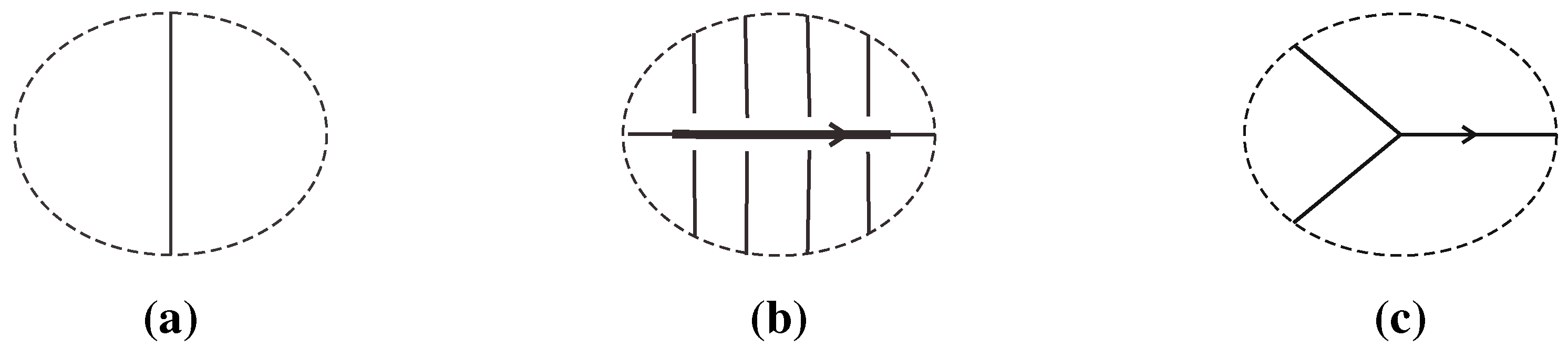
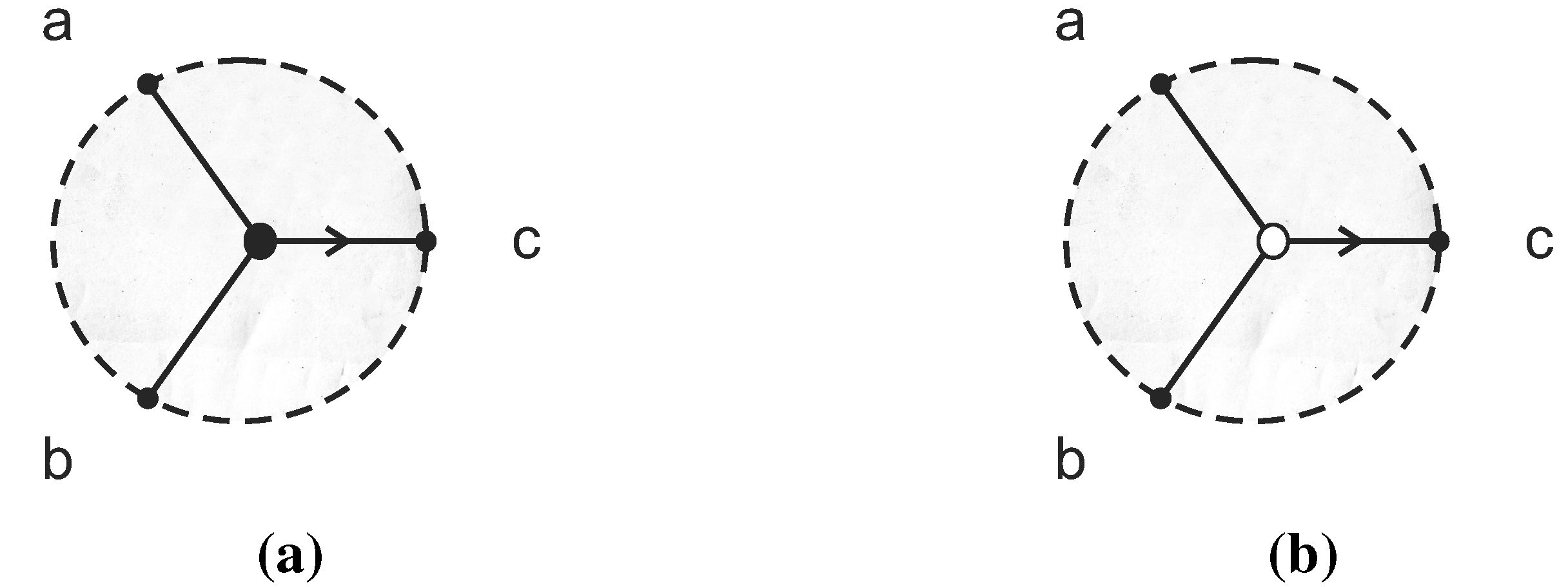
We define here a tangle machine, without colors, to be a diagram that occurs by concatenating (connecting endpoints) of a finite number of generators of the form in Figure 3. Thickened lines in interactions (Figure 3b) are called agents, and each thin line is called a patient. Only agents are directed, and their is no compatibility condition between the directions of different agents.

Figure 3. Generators for tangle machines are struts and interactions. Generators for trivalent tangle machines are struts, interactions and wyes. (a) strut; (b) interaction; (c) wye.

Figure 3. Generators for tangle machines are struts and interactions. Generators for trivalent tangle machines are struts, interactions and wyes. (a) strut; (b) interaction; (c) wye.

Arcs in a tangle machine, ending as under-arcs passing under an agent or at a wye or at a machine endpoint (thus “continuing right through agents”), are called registers. Later on, registers will contain colors.

Tangle machines have struts and interactions as generators, whereas trivalent tangle machines have struts, interactions and wyes as generators. An example of a machine constructed by concatenation is presented in Figure 4. As in the theories of virtual knots and of w-knotted objects, concatenation lines may intersect [35,36]. Furthermore, as in the theory of disoriented tangles, no compatibility condition is imposed for directions of concatenated agents [37].

Figure 4. Concatenation of tangle machines.

Figure 4. Concatenation of tangle machines.

3.2. Colors

Let Q be a set equipped with a family B of binary operations that satisfy the following three axioms:

• Idempotence: $x▹x=x$ for all $x\in Q$ and for all $▹\in B$.
• Reversibility: The map $▹y:Q\to Q$, which maps each color $x\in Q$ to a corresponding color $x▹y\in Q$, is a bijection for all $(y,▹)\in (Q,B)$. In particular, if $x▹y=z▹y$ for some $x,y,z\in Q$ and for some $▹\in B$, then $x=z$.
• Distributivity: For all $x,y,z\in Q$ and for all $▹\in B$:

  $$(x▹y)▹z=(x▹z)▹(y▹z).$$

  (4)

Remark 2. Reversibility may be weakened by requiring only that $▹y$ be an injection for all y, but not necessarily a surjection. This is indeed the case for the machines that we describe in the context of interactive proofs.

The pair $(Q,B)$ is called a quagma. It is called a quandle if the operations in B distribute over one another, in the sense that:

$$(x▹y)▸z=(x▸z)▹(y▸z),$$

(5)

for all $▹,▸\in B$. This definition is a variant of definitions found in [38,39,40]. If we weaken reversibility to require only that $▹y$ be an injection for all $y\in Q$ and for all $▹\in B$, the resulting structure is called a quandloid [4]. Quagmas, quandloids and quandles serve as the content of registers in tangle machines.

Example 1 (Conjugation quandle). Colors might be elements of a group Γ, and the operation might be conjugation:

$$x▸y=y^{-1}xy.$$

(6)

The pair $(\Gamma ,\left\{▸\right\})$ is called a conjugation quandle. Such quandles feature in knot theory, e.g., [41].

Example 2 (Linear quandle). Colors might be real numbers, and the operations might be convex combinations:

$$x{▹}_{s}y=(1-s)x+sys\in \mathbb{R}\backslash \left\{1\right\}.$$

(7)

The pair $\left(Q,{\left\{{▹}_s\right\}}_{s\in \mathbb{R}}\right)$ is called a linear quandle.

3.3. With Colors

A coloring of a tangle machine M is an assignment ϱ of a binary operation in B to each agent and an assignment ρ of an element of Q to each register, such that, at each interaction, the color $z\in Q$ of the patient to the right of the agent (according to the right-hand rule) equals the color of its corresponding patient to the left of the agent $x\in Q$ right-acted on by the color of the agent $y\in Q$ via the operation of the agent $▹\in B$:

(8)

Thus, an interaction “realizes” the action of the quagma or of the quandle.

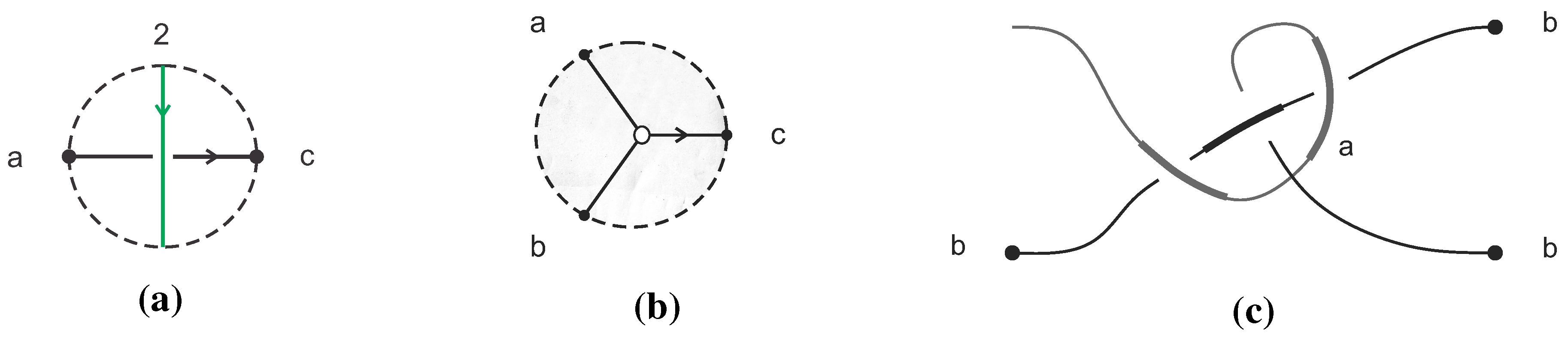
To color a trivalent tangle machines, Q has to come equipped with a complete ordering. We include also an assignment of either max or min to each wye, so that the exiting register of the wye is the maximum of the two inputs if the wye is labeled max and is their minimum otherwise. We graphically denote a min label with a white circle at the branch-point of the wye and a max label by a black circle. See Figure 5.

Figure 5. Coloring wyes colored by max and min.

Figure 5. Coloring wyes colored by max and min.

Remark 3. The notion of the tangle machine given above is more general than in [1,4], in which all tangle machines are quandle-colored and without wyes.

Finally, we come to the notion of a tangle machine computation.

Definition 6. A computation of a (trivalent) tangle machine M is:

1.

A choice of a set $S_{\mathit{in}}$ of input registers in M.

2.

A choice of a set $S_{\mathit{out}}$ of output registers in M with $S_{\mathit{in}}\cap S_{\mathit{out}}=\varnothing$.

3.

A coloring ϱ of all agents in M (and an assignment of either max or min to each wye).

4.

A coloring ${\rho }_{\mathit{in}}$ of all registers in $S_{\mathit{in}}$.

5.

A unique (oracle) determination of a coloring ${\rho }_{\mathit{out}}$ of all registers in $S_{\mathit{out}}$. If ${\rho }_{\mathit{in}}$ does not uniquely determine ${\rho }_{\mathit{out}}$, the computation cannot take place.

4. Tangle Machines Are Turing Complete

Our goal in this section is to realize the universal set of gates, $\mathrm{NOT}(\neg )$ and $\mathrm{AND}(\wedge )\}$, as well as a multiplexer that duplicates the content of a register, using tangle machines. This realizes the Boolean circuit model, thus showing that tangle machines are Turing complete.

Remark 4. A tangle machine computation, which is based on an oracle, which tells us the colors of output registers given colors of input registers, can carry out super-Turing computations. Consider the conjugation quandle of a group Γ with unsolvable conjugacy problem and color agents ${\mathrm{In}}_1$ and ${\mathrm{In}}_2$ by elements of Γ. The color of Out might not be Turing computable, but the tangle machine computation computes it.

(9)

4.1. Quagma Approach

Choose the set of colors to be $Q\stackrel{\mathrm{def}}{=}{\mathbb{Q}}^{2\times 2}$, equipped with a set B of binary operations whose elements are the following:

$$X▸Y=\left\{\begin{array}{cc}{Y}^{-1}XY,\hfill & \text{if}det\left(Y\right)\ne 0\text{;}\hfill \\ X,\hfill & \text{otherwise.}\hfill \end{array}\right.$$

(10)

$$X{▹}_{s}Y=(1-s)X+sY,\text{for}s=\frac{1}{2}\text{or}s=2\text{.}$$

(11)

The structure $(Q,\{{▹}_{0.5},{▹}_2,▸\})$, henceforth referred to simply as Q, is a quagma.

To realize Boolean logic, let $A_0\stackrel{\mathrm{def}}{=}\left(\begin{array}{cc}0& 1\\ 1& 0\end{array}\right)$ and $A_1\stackrel{\mathrm{def}}{=}\left(\begin{array}{cc}1& \phantom{-}0\\ 0& -1\end{array}\right)$ stand in for the digits zero and one, correspondingly. Incidentally, these happen to coincide with the Pauli spin matrices of quantum mechanics.

A NOT gate is described by a single interaction:

(12)

where the respective truth-table is shown to the right of the diagram. Explicitly,

$$\neg X=X▸(A_0+A_1)={\left(\begin{array}{cc}1& \phantom{-}1\\ 1& -1\end{array}\right)}^{-1}X\left(\begin{array}{cc}1& \phantom{-}1\\ 1& -1\end{array}\right)=\frac{1}{2}\left(\begin{array}{cc}1& \phantom{-}1\\ 1& -1\end{array}\right)X\left(\begin{array}{cc}1& \phantom{-}1\\ 1& -1\end{array}\right)$$

(13)

The input is the register labeled X; the output is the register labeled $\neg X$; and the remaining register is always colored by the constant value $A_0+A_1$.

Realizing an AND gate can be split into several successive computations, let X and Y be the inputs to the gate, and write $\mathbf{0}$ for $\left(\begin{array}{cc}0& 0\\ 0& 0\end{array}\right)$. The following instructions end up with the desired operation $X\wedge Y$.

• ${\beta }_1=(A_0+A_1)▸\left(X{▹}_{{}_{0.5}}Y\right)={(X+Y)}^{-1}(A_0+A_1)(X+Y)$
• ${\beta }_2={\beta }_1{▹}_{{}_{0.5}}(A_0+A_1)=\frac{1}{2}{\beta }_1+\frac{1}{2}(A_0+A_1)$
• ${\beta }_3=({\beta }_2▹A_0){▹}_{{}_{0.5}}{\beta }_2=\frac{1}{2}{A}_0{\beta }_2{A}_0+\frac{1}{2}{\beta }_2$
• $X\wedge Y=A_1▸\left({\beta }_3{▹}_{{}_{0.5}}{A}_1\right)={({\beta }_3+A_1)}^{-1}{A}_1({\beta }_3+A_1)$

A tangle machine that realizes these steps is given below together with the respective truth-table.

(14)

$$\begin{array}{cccccc}X& Y& {\beta }_1& {\beta }_2& {\beta }_3& X\wedge Y\\ A_0& A_0& A_0-A_1& A_0& A_0& A_0\\ A_0& A_1& A_0+A_1& A_0+A_1& A_0& A_0\\ A_1& A_0& A_0+A_1& A_0+A_1& A_0& A_0\\ A_1& A_1& A_1-A_0& A_1& \mathbf{0}& A_1\end{array}$$

(15)

In addition to the universal set of gates, we also need to be able to duplicate the content of a register. The conventional Boolean circuit model includes junction points along wires. The tangle machine analogue for such a junction is a multiplexer, that is a machine whose output colors are duplicates of the color in one of its inputs. A multiplexer takes an input of the form $\{X,\underset{n-1\text{times}}{\underbrace{0,\dots ,0}}\}$ and outputs $\{\underset{n\text{times}}{\underbrace{X,\dots ,X}}\}$. The operation of a multiplexer is captured by the machine in Figure 6.

Figure 6. A multiplexer.

Figure 6. A multiplexer.

Remark 5. Two fundamental properties of quantum information are no-cloning and no-deleting. The uniform version of no-cloning states that there does not exist a unitary operator C for which $C(A\otimes e)C^{†}=A\otimes A$ for all states A, where e denotes the identity operator. The uniform version of no-deleting states that there does not exist a unitary operator U for which $U(A\otimes A)U^{†}=A\otimes e$ for all states A. Both of these statements are captured by the quagma axioms. Consider the quagma $(Q,\left\{{▹}_{0.5},▸\right\})$ where Q is the set of invertible operators and ▸ is any binary operation that distributes over ${▹}_{0.5}$, e.g., conjugation. If U were a universal cloning operator with respect to ▸, i.e., if $(A\otimes e)▸U=A\otimes A$ for all A, then for any state A, both machines in Figure 7 would carry out the same computation and, in particular, ${\mathrm{Out}}_1={\mathrm{Out}}_1^{\prime }$. However, then, $\left(A{▹}_{0.5}B\right)\otimes \left(A{▹}_{0.5}B\right)={\mathrm{Out}}_1={\mathrm{Out}}_1^{\prime }=(A\otimes A){▹}_{0.5}(B\otimes B)$, which is false in general. Thus, universal cloning violates distributivity. No-deleting follows from no-cloning, because if U were a universal deleting operator with respect to ▸, then U would also be a universal cloning operator with respect its inverse operation ◂, which exists thanks to reversibility. This would violate distributivity, because ◂ also distributes over ${▹}_{0.5}$, as can be seen by applying $◂Z$ to both sides of the equation:

$$X{▹}_{0.5}Y=\left((X◂Z){▹}_{0.5}(Y◂Z)\right)▸Z.$$

We parenthetically note that no-cloning and no-deleting are also captured by a different diagrammatic calculus, that of categorical quantum mechanics [42].

Figure 7. Universal cloning violates distributivity.

Figure 7. Universal cloning violates distributivity.

4.2. Wye Approach

Realizing a universal set of logic gates is easier if we allow wyes and may be realized with a quandle coloring.

We color our machines by elements of the quandle $Q\stackrel{\mathrm{def}}{=}\{0,1,2\}$ subject to the quandle operation $x▹y=2y-xmod3$ (this is a Fox three-coloring). We totally order Q by $0<1<2$. Color-code 0 as red, 1 as blue and 2 as green. For this particular quandle the direction of the agent does not matter because the operation ▹ is its own inverse. Let 0 stand in for the digit zero and 1 stand in for the digit one. A universal set of logic gates and a multiplexer can be obtained as in Figure 8, where an incoming arrow represents input and an outgoing arrow represents output.

4.3. Nonabelian Simple Group Approach

The AND gate constructed in Section 4.1 was realized as a tangle machine colored by a quagma, which is not a quandle, and the AND gate of Section 4.2 used a wye. In fact, it is possible to realize a universal set of logic gates with a conjugation quandle colored tangle machine without using wyes.

Figure 8. Logic gates for the three-color approach. Inputs are the colors on the left, and outputs are colors on the right. (a) NOT gate; (b) AND gate; (c) multiplexer.

Figure 8. Logic gates for the three-color approach. Inputs are the colors on the left, and outputs are colors on the right. (a) NOT gate; (b) AND gate; (c) multiplexer.

The construction is based on Barrington’s theorem [43,44]. Following [16], Appendix A of [17] constructs a 132 crossing 14 strand braid colored by the conjugation quandle of the finite simple group $A_5$, which realizes the Toffoli gate that is a universal logic gate [45]. This braid is made a tangle machine by interpreting each crossing as an interaction. Three of its registers are inputs; three are outputs; and it contains a number of ancilla, which are what we called control registers.

5. Turing Machine Simulation

In this section, we show how to simulate a Turing machine using a tangle machine.

5.1. Turing Tangle Machine

In this section, we make use of the linear quandle whose underlying set of elements Q is the set of the rational numbers and whose set of operations B is:

$$x{▹}_{s}y=(1-s)x+sys\in \mathbb{Q}\backslash \left\{1\right\}.$$

(16)

There are several sub-machines that recur in the construction of a Turing tangle machine, the tangle machine analog of a Turing machine. To simplify our diagrams, we represent these sub-machines graphically.

Multiplexer We indicate a multiplexer by splitting a strand.

(17)

The multiplexer is realized by composing diagrams of the form in Figure 6.

Negation $\neg x\stackrel{\mathrm{def}}{=}1-x$.

(18)

Addition

(19)

Indicator If $x\ge 1$ then$ı\left(x\right)=1$, if $0<x<1$, then $ı\left(x\right)=x$, otherwise $ı\left(x\right)=0$.

(20)

Beta A function $\beta \left(x\right)$, which satisfies $\beta \left(0\right)=-1$, $\beta \left(\frac{1}{2}\right)=0$ and $\beta \left(1\right)=1$.

(21)

• Selector Depending on the color c of a control strand, either x or y emerges as the output, z. To be precise, $z=x$ if $c=0$, and $z=y$ if $c=1$.

  (22)

  where s is an arbitrary constant whose value is greater than two.

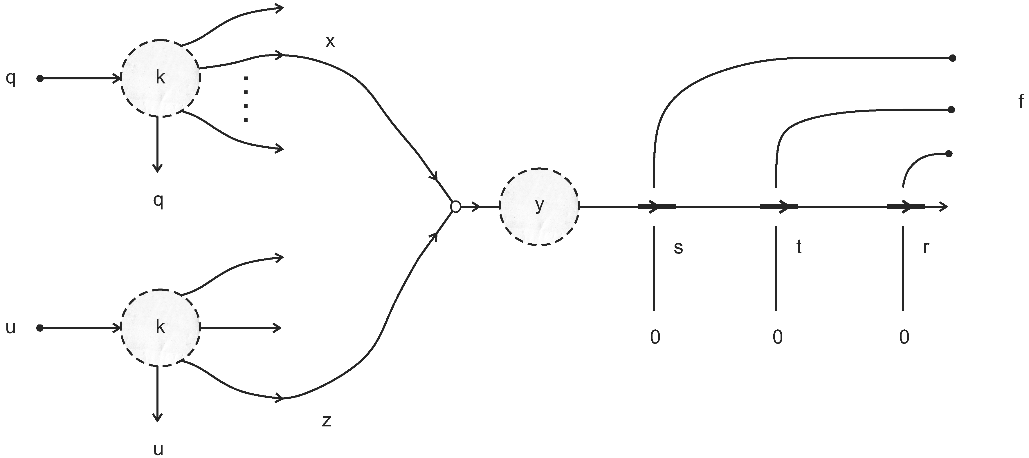
• Mask-generating machine This sub-machine is shown in Figure 9. Its input registers are a register colored by an integer $p\in Q$, called a pointer, and a sequence of colored registers together, called a mask. Its output registers are a register colored p, and one register colored zero for all other input colored registers, except for a single register colored one in the p-th position of the output.

Figure 9. A mask-generating machine.

Figure 9. A mask-generating machine.

5.2. Finite Control

The first step in realizing a Turing machine is to mimic the finite control unit, i.e., to simulate the transition function:

$$\delta \left(q\right(k),u(k\left)\right)=\left(q\right(k+1),a,ϵ)$$

(23)

Given the current machine state $q\left(k\right)$ and the symbol currently under the R/W head $u\left(k\right)$, the transition function determines the next machine state $q(k+1)$ together with a pair of tape instructions: the symbol to be written a and an ϵ movement of the head to its next position along the tape. Without loss of generality, we shall assume henceforth that the finite control states are all natural numbers and, in particular, that $\mathit{S}=\left\{1,\dots ,n\right\}$.

The basic building block of the finite control tangle machine is a hardwired transition, that is a function ${\delta }_{i,j}:\mathit{S}\times \Sigma \to {\mathbb{Z}}^3$,

$$(q,u)\mapsto \left\{\begin{array}{cc}(\overline{q}+2,\overline{a}+2,\overline{ϵ}+2),\hfill & \text{if}q=i\text{and}u=j+1\text{;}\hfill \\ (-\overline{q}-2,-\overline{a}-2,-\overline{ϵ}-2),\hfill & \text{otherwise.}\hfill \end{array}\right.$$

(24)

where $\overline{q},\overline{a},\overline{ϵ}$ denote, respectively, the next assumed state and the tape instructions as specified in the definition of ${\delta }_{i,j}$. The parameters $i,j$ and the respective output of ${\delta }_{i,j}$, the triplet $(\overline{q},\overline{a},\overline{ϵ})$, are hardwired into the tangle machine realization of ${\delta }_{i,j}$ through the quandle parameters. See Figure 10.

Figure 10. Hardwired transition.

Figure 10. Hardwired transition.

The hardwired transition is symbolically represented as:

(25)

The transition function δ is constructed by combining several hardwired transitions. Note that there are no more than $3n$ possible transitions in the finite control (n states multiplied by three input symbols). Thus, the number of distinct binary operations in B does not exceed $9n+\mathcal{O}\left(1\right)$, which accounts for $3n$ triplets $({▹}_{\overline{q}+2},{▹}_{\overline{a}+2},{▹}_{\overline{ϵ}+2})$ and a few other operations required for realizing the memory unit. A detailed construction of the finite control sub-machine is shown in Figure 11.

Figure 11. A tangle machine realization of a finite control unit.

Figure 11. A tangle machine realization of a finite control unit.

5.3. Memory Unit and One-Step Computation

The memory unit consists mainly of the tape logic. It accepts a finite, possibly unbounded set of registers whose colors are manipulated in the basis of commands a and ϵ received from the finite control. The majority of the registers of the memory unit correspond to tape cells whose content is represented by colors from the set Σ.

We construct the memory (tape) reading and writing operations using a mask-generating machine together with selector machines to output the color of the $p\left(k\right)$-th register, either as it originally appeared or modified. See Figure 12.

Figure 12. Memory reading and writing sub-machines. Here, $\frac{1}{2}<s<1$ is an arbitrary parameter. (a) Write; (b) read.

Figure 12. Memory reading and writing sub-machines. Here, $\frac{1}{2}<s<1$ is an arbitrary parameter. (a) Write; (b) read.

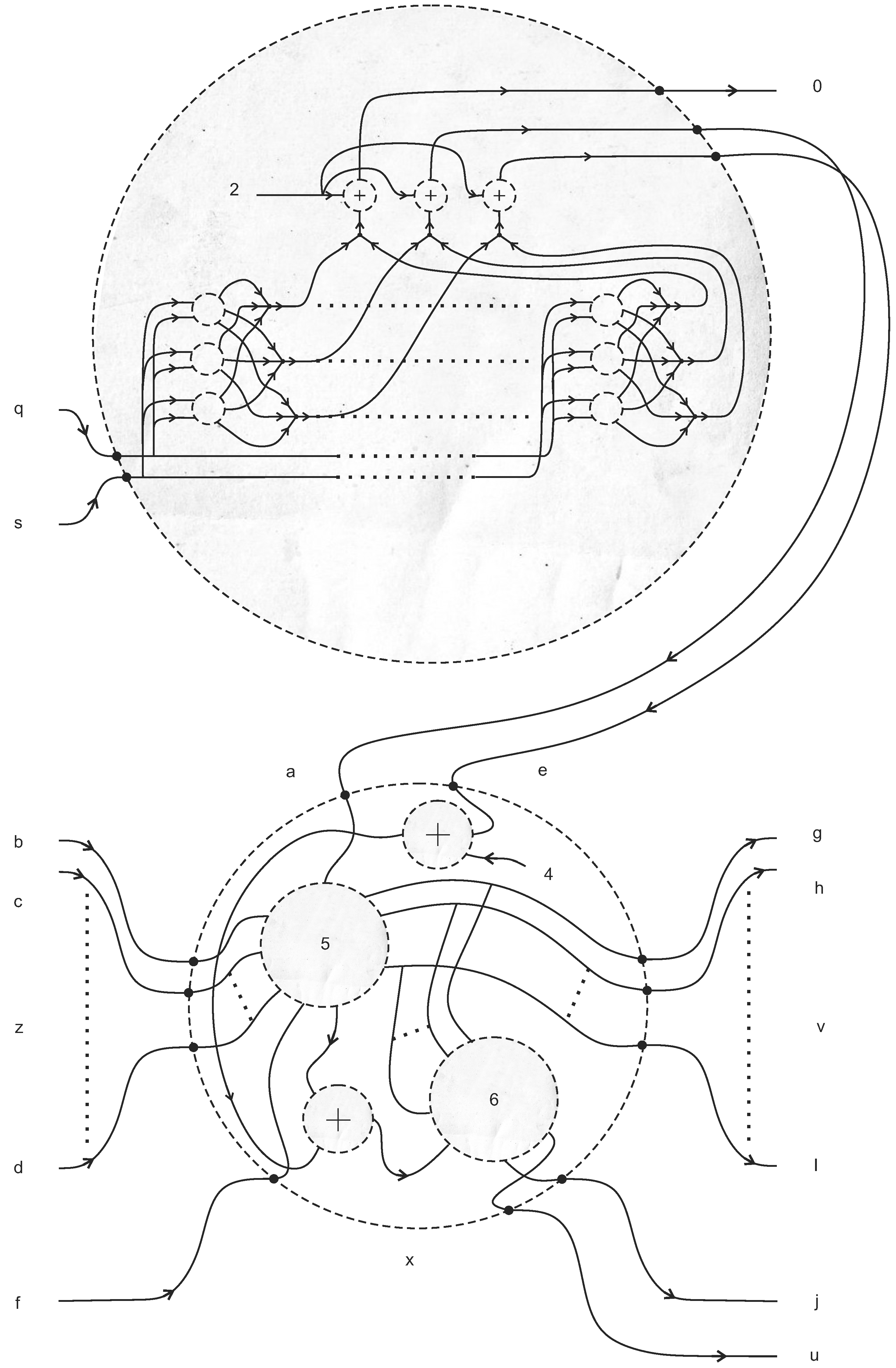
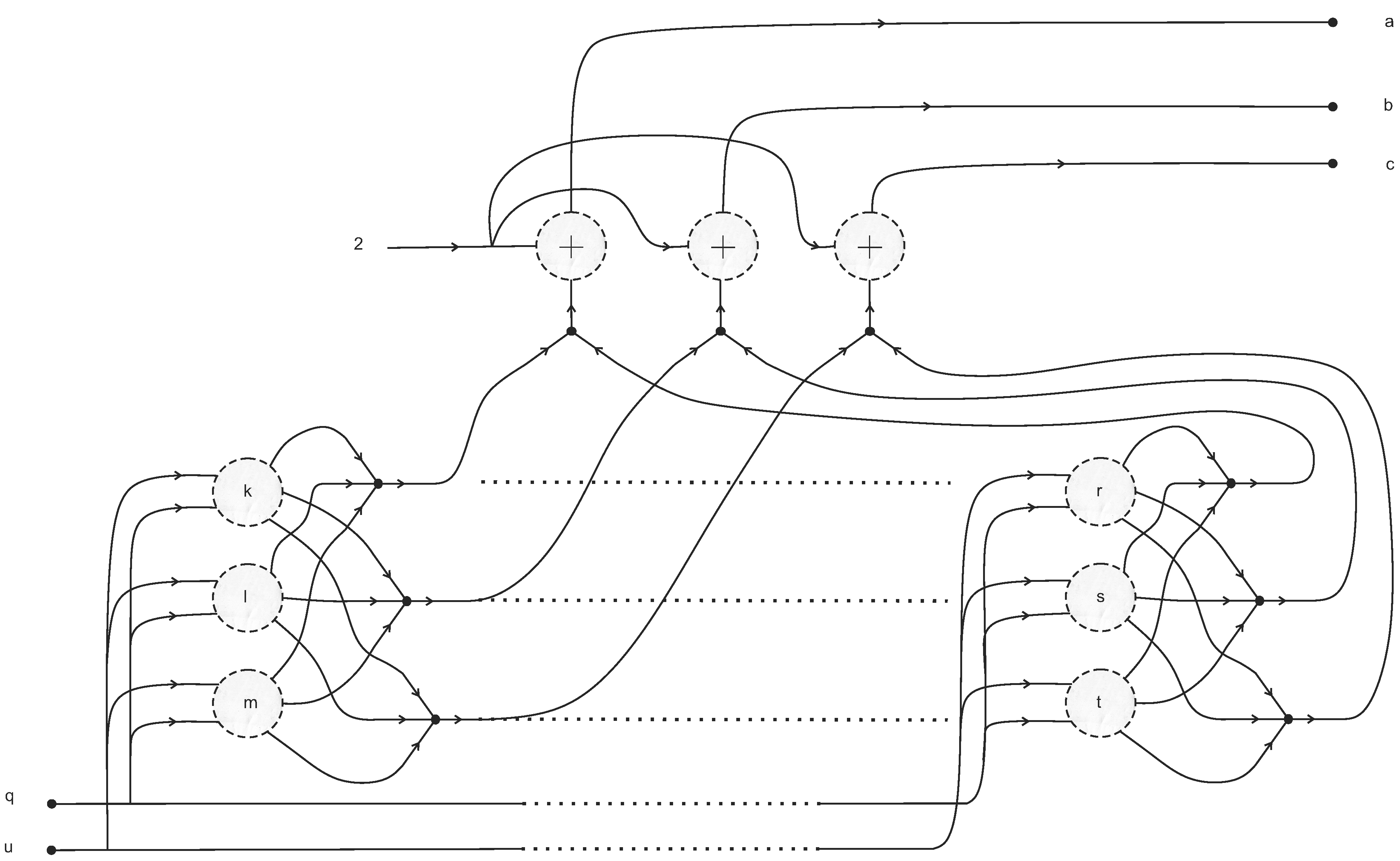
Figure 13 illustrates the memory unit, connected to the finite control unit. Its inputs are:

• An integer pointer register colored $p\left(k\right)$, indicating the current head position.
• A finite, possibly unbounded set of registers, each of which represents a single (memory) cell on a tape. These tape registers are colored ${\left\{c_i\left(k\right)\right\}}_{i>0}\in \Sigma$.
• A pair of registers colored correspondingly by a pair instructions $(a,ϵ)$, where a denotes the symbol to be written in the current cell to which the head points (which is numbered $p\left(k\right)$), and ϵ denotes the (possibly zero) increment to be added to $p\left(k\right)$, so that $p(k+1)=p\left(k\right)+ϵ-1$.

The outputs of the memory unit are:

• The updated pointer $p(k+1)$.
• A finite, possibly unbounded set of registers whose colors ${\left\{c_i(k+1)\right\}}_{i>0}\in \Sigma$ have been all passed unchanged, except for a single cell whose content may have been modified.
• A strand colored by $u(k+1)$, the content of the cell to which the head points in its new location $p(k+1)$

Figure 13. One-step computation of a Turing tangle.

Figure 13. One-step computation of a Turing tangle.

To simulate the sequential operation of a Turing machine, copies of the finite control unit and of the memory unit are to concatenated in the obvious manner. Concatenating N copies of the machine in Figure 13 simulates N successive computations of a Turing machine (see Figure 14). This justifies naming such a procedure iteration.

Figure 14. Iterative computation in a Turing tangle machine.

Figure 14. Iterative computation in a Turing tangle machine.

5.4. Halting

A halting state is a state for which:

$$\delta (q_h,u)=(q_h,u,1)$$

(26)

Once arriving at a halting state, further iterations do not alter the memory content of the machine. The state $q_h$ represents an equilibrium, which may or may not be reached for a given input sequence $u\left(0\right),u\left(1\right),\dots$. A machine whose input registers are colored by a halting state can be closed by concatenating respective inputs and outputs, as shown in Figure 15.

Figure 15. Closure of a Turing tangle machine in its halting state.

Figure 15. Closure of a Turing tangle machine in its halting state.

6. Interactive Proofs: Distribution of Knowledge by Deformation

The decision of a crowd can converge to a correct answer even when each individual has limited knowledge. This phenomenon is known as the wisdom of the crowds [46]. In line with “the many being smarter than the few”, we extend the notion of interactive proof systems [26] to a system in which a collection of verifiers interact to prove a claim together. Might such a crowd of verifiers collaborate to prove more than could be proven by any individual verifier in the crowd?

6.1. Deformation of a Single Interaction

Consider a family of verifiers, each with a belief concerning whether $x\in L$ or $x\notin L$. We model the belief of each verifier W at time t as a Bernoulli random variable $W_t$ whose realizations $w_t$ are either $\left|\mathrm{True}\right)$ or $\left|\mathrm{False}\right)$. We interpret $w_t=\left|\mathrm{True}\right)$ as “W believes at time t that $x\in L$”, and we interpret $w_t=\left|\mathrm{False}\right)$ as “W believes at time t that $x\notin L$”.

Consider an interaction at time t with agent V, one of whose patients is W. The realization $w_{t+1}$ of $W_{t+1}$ may equal either the belief of the agent $v_t$ or the belief of the patient $w_t$. In other words, W either retains her belief or is “convinced” by V to change her belief to that of V (we use female pronouns for the verifiers, who are all “Alices”). Whether or not V “succeeds in convincing W” depends on a message ${\xi }_t$ from a prover Π with access to an oracle.

Only the belief of patients changes at an interaction. The agents and the verifiers who do not participate in the interaction do not change their beliefs, so in particular, $v_{t+1}=v_t$ always.

There are three constants associated with the agent V at an interaction at time t: a completeness parameter $c_V^t$, a soundness parameter $s_V^t$ with $0<s_V^t<c_V^t\le 1$, and a deformation parameter ${\delta }_V^t\in \mathbb{Q}\cap (0,1)$. For simplicity, we will assume that these three parameters are the same for all agents in the network, and $s_v^t,c_V^t,{\delta }_V^t$ will be written $s,c,\delta$ correspondingly.

Our basic requirement for an interaction is that the following pair of inequalities be satisfied:

$$\begin{array}{cc}\text{(deformed}\text{completeness)}\hfill & x\in L⟶Pr(W_{t+1}=v_t\mid V_t=v_t)\ge c\delta ;\hfill \\ \text{(deformed}\text{soundness)}\hfill & x\notin L⟶Pr(W_{t+1}=v_t\mid V_t=v_t)\le s\delta .\hfill \end{array}$$

(27)

Remark 6. The deformed completeness and soundness, $c\delta$ and $s\delta$, may both be below $\frac{1}{2}$ or may both be above $\frac{1}{2}$ and bounded away from one.

In the limit $\delta \to 1$, specific values of c and of s turn the pair of inequalities Equation (27) into familiar pairs of inequalities in interactive proof theory [47]. For example, for $s=2^{-{\left|x\right|}^a}$ and $c=1-2^{-{\left|x\right|}^b}$, where $a,b>0$, we obtain the completeness and soundness constraints of an IP verification.

6.2. Statistics of Beliefs and Interactions

When keeping track of the beliefs of many different verifiers at many different times, it is cumbersome to work directly with Equation (27). Instead, we introduce a shorthand to keep track of the belief of a verifier, both if $x\in L$ and also if $x\notin L$, in a single expression.

The belief statistics $\left|W_t\right)$ of verifier W at time t is written:

$$\left|W_t\right)\stackrel{\mathrm{def}}{=}a\left|\mathrm{True}\right)+b\left|\mathrm{False}\right),$$

(28)

where $a\in [0,1]$ denotes the greatest lower bound for the belief of W that $x\in L$ at time t conditioned on this belief indeed being true, and $b\in [0,1]$ denotes the greatest lower bound for the belief of W that $x\notin L$ at time t conditioned on this opposite belief indeed being true. Note that $a+b$ need not equal one. In particular:

$$\begin{array}{cc}x\in L\hfill & ⟶a\le Pr(W_t=\left|\mathrm{True}\right));\hfill \\ x\notin L\hfill & ⟶b\le Pr(W_t=\left|\mathrm{False}\right)).\hfill \end{array}$$

(29)

An interaction between W and V at time t concludes either with W accepting the belief of V or with W sticking to her own belief. Denoting by h the probability (or more precisely, a lower bound on it) of W switching to the belief of V in the next time frame, the distribution of possible beliefs of W in the next time frame is described by:

$$\left|W_{t+1}\right)={\left|W_t\right)}^{\left|V_t\right)}\stackrel{\mathrm{def}}{=}(1-h)\left|W_t\right)+h\left|V_t\right).$$

(30)

Remark 7. Belief statistics written as in Equation (28) facilitate calculations of probabilities across a network. This tool is used throughout the remainder of this note (some examples will be given shortly). Here, we explain how Equations (28) and (30) combine to give a compact way of representing two entirely different interactions, one assuming $x\in L$ and the other assuming $x\notin L$. This may be slightly confusing at first, so the reader’s attention is called to this point.

Owing to Equation (30), the probabilities anywhere in the network at time $t>0$ depend on the parameter h. We may do all calculations and treat it as a formal parameter. Having in mind that an interaction is ultimately a procedure terminating with the statistics in Equation (27), the parameter h is set either to $c\delta$ or to $s\delta$ depending on whether or not x is in L. To verify that a network decides L, we repeat the computation twice, first for the case where $x\in L$ and then for $x\notin L$. In the former case, we will be interested only in the coefficient of $\left|\mathrm{True}\right)$, whereas in the latter case, we will be interested only in the coefficient of $\left|\mathrm{False}\right)$.

Here is an illustrative calculation for a single interaction. Let $W_t=\left|\mathrm{False}\right)$ and $V_t=\left|\mathrm{True}\right)$. Invoke Equation (30) using the completeness and soundness parameters in Equation (27): first using $h=c\delta$ and then using $h=s\delta$. Hence,

$$\left|W_{t+1}\right)=c\delta \left|\mathrm{True}\right)+(1-s\delta )\left|\mathrm{False}\right)⟶\left\{\begin{array}{cc}c\delta \left|\mathrm{True}\right)+(\cdots )\left|\mathrm{False}\right),\hfill & x\in L;\hfill \\ (\cdots )\left|\mathrm{True}\right)+(1-s\delta )\left|\mathrm{False}\right),\hfill & x\notin L.\hfill \end{array}\right.$$

(31)

This interaction is said to decide L only if $c\delta >\frac{1}{2}$ and $1-s\delta >\frac{1}{2}$.

6.3. Expressive Power of a Network: The Class BraidIP

Verifiers in our framework are assumed to be implemented as probabilistic polynomial-time Turing machines whose beliefs are either internal states or are stored on tapes. Similarly, an interaction is a polynomial-time procedure. Consider now a crowd of verifiers $V^1,V^2,\dots ,V^{\mu }$ whose initial beliefs at time $t=0$ are $\left|V_0^1\right),\left|V_0^2\right),\dots ,\left|V_0^{\mu }\right)$. Allow them to interact at times $t=0,1,2,\dots ,\chi$, subject to parameters $0<c<s\le 1$ and $\delta \in \mathbb{Q}\cap (0,1)$. We write M for this sequence of interactions. A language $L\subseteq {\{0,1\}}^{*}$ is said to be decided by M if M contains a verifier V, whose belief at time χ is $\left|V_{\chi }\right)\stackrel{\mathrm{def}}{=}a\left|\mathrm{True}\right)+b\left|\mathrm{False}\right)$, such that, for a fixed constant $\kappa >0$, we have:

$$\begin{array}{c}x\in L⟶a\ge \frac{1}{2}+{\left|x\right|}^{-\kappa };\hfill \\ x\notin L⟶b\ge \frac{1}{2}+{\left|x\right|}^{-\kappa }.\hfill \end{array}$$

(32)

This definition depends on the choice of $\kappa >0$. The class braided interactive polynomial time (BraidIP) consists of those languages that are decidable for any fixed $\kappa >0$ by some network M in time χ, polynomial in $\left|x\right|$. We denote this class $\mathrm{BraidIP}\{\delta ,\chi \}$, where χ is the number of interactions in M.

Remark 8. The definition of class BraidIP is similar in spirit to the class BPP. We will see below that it includes class IP. Letting Equation (32) reflect the class PP (i.e., taking strict inequalities and right-hand constants equal to $\frac{1}{2}$) will result in networks that decide any $L\in \mathrm{IPP}$.

6.4. Braid of Beliefs

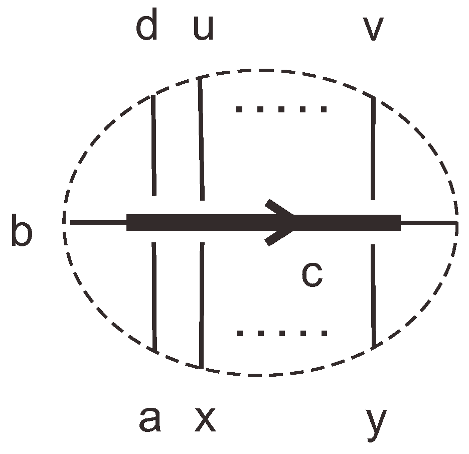
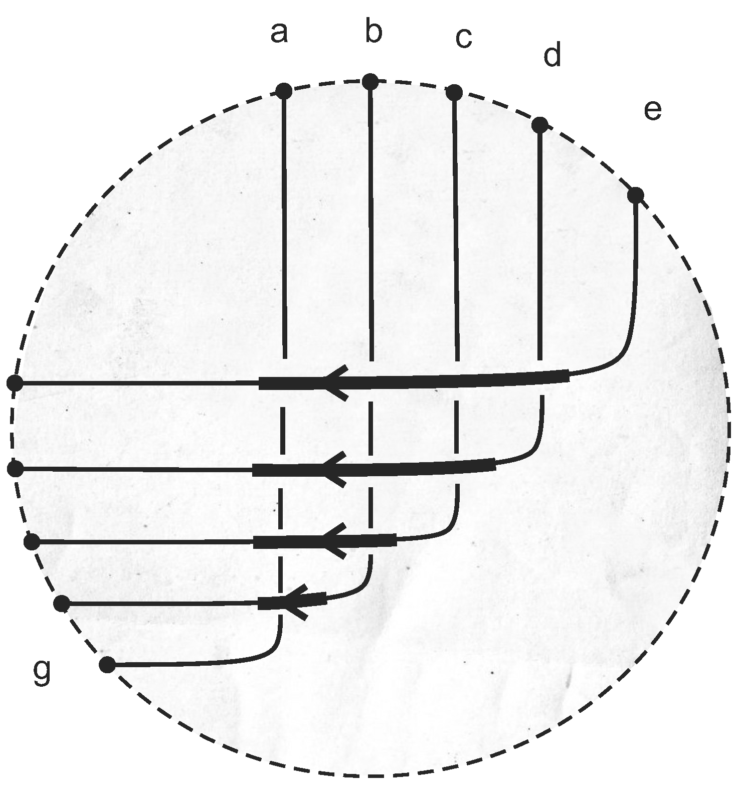
Our networks admit a convenient diagrammatic description. We represent an interaction as a wire cutting through other wires (see Figure 16). The overcrossing wire, which becomes slightly thickened in an interaction, carries the belief statistics of an agent, whereas the undercrossing wires carry the belief statistics of her patients. An example of many concatenated interactions is given in Figure 17.

Figure 16. Diagrammatic representation of an interaction.

Figure 16. Diagrammatic representation of an interaction.

Figure 17. A rumor-passing network and its respective diagram.

Figure 17. A rumor-passing network and its respective diagram.

The diagram representing the rumor passing network in Figure 17 is a braid, which is a special sort of tangle. Here, such diagrams represent the flow of beliefs within a network of interacting machines (verifiers).

When many patients pass under a single agent, we define this to imply that for each patient, the belief sampled from that patient is independent of the belief sampled from every other patient, and the belief sampled from the agent to update that patient’s belief is independent of the belief sampled from the agent to update every other agent’s belief. To say the same thing in a different way, multiple patients under the same agent are independent and unsynchronized during that time frame. We will discuss this point further in Section 10.2.

6.5. An Example

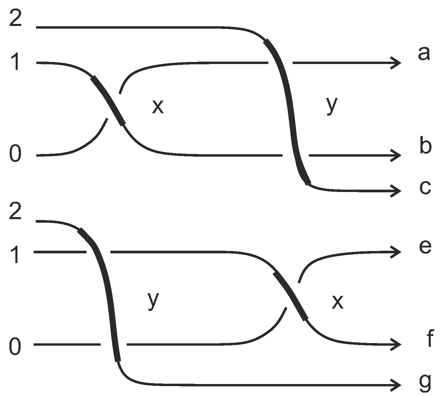
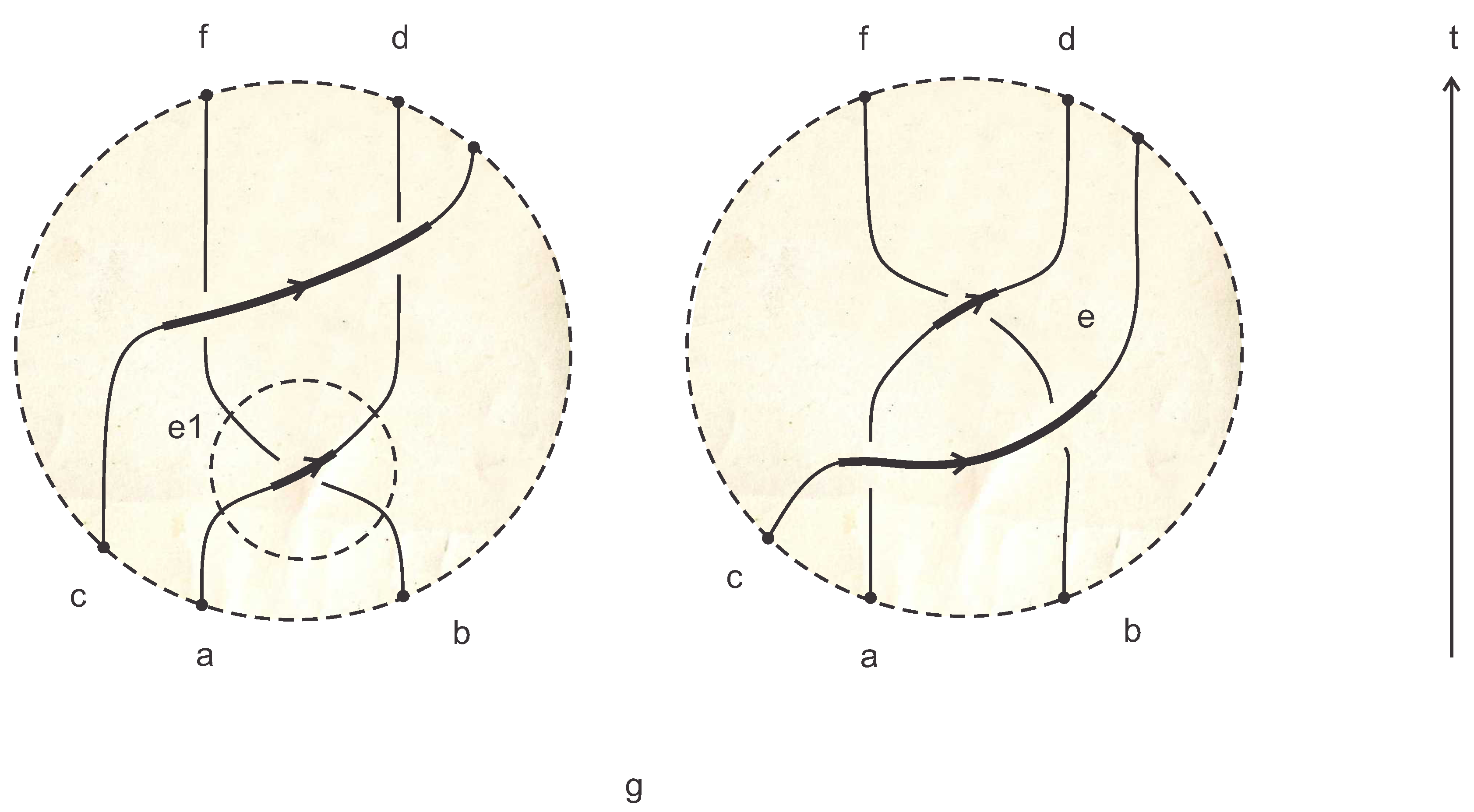
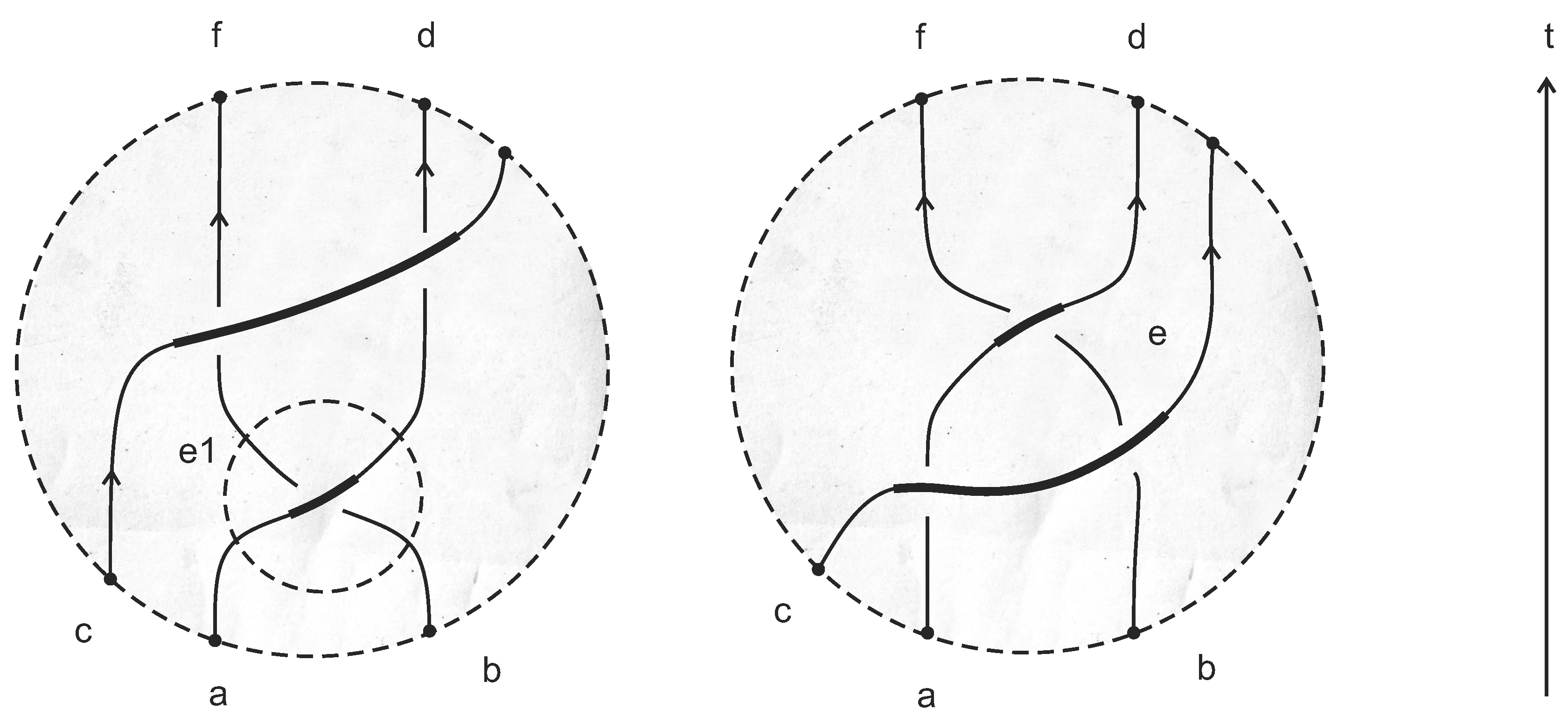
The capacity of a network to prove or disprove a claim is an emergent property. Out of a number of uncertain interactions, none of which prove the claim, the truth may eventually materialize. As an example, consider the two pairs of two consecutive interactions pictured in Figure 18. Both sequences involve three verifiers, designated X, Y and Z. Their initial beliefs are shown at the bottom.

Figure 18. Equivalent networks of interactions.

Figure 18. Equivalent networks of interactions.

Set the parameters to $s\stackrel{\mathrm{def}}{=}\frac{1}{2}$, $c\stackrel{\mathrm{def}}{=}1$ and $\delta \stackrel{\mathrm{def}}{=}\frac{1}{2}$. Allow the verifiers to interact in the left diagram. At time $t=2$, beliefs $X_0$ and $Y_0$ of X and of Y have been updated to $X_2$ and to $Y_2$ (Z does not change his belief). The distributions are:

$$\left|X_2\right)={\left({\left|X_0\right)}^{\left|Y_0\right)}\right)}^{\left|Z_0\right)}⟶\left\{\begin{array}{cc}\frac{3}{8}\left|\mathrm{False}\right)+\frac{5}{8}\left|\mathrm{True}\right),\hfill & x\in L;\hfill \\ \frac{21}{32}\left|\mathrm{False}\right)+\frac{11}{32}\left|\mathrm{True}\right),\hfill & x\notin L.\hfill \end{array}\right.$$

(33)

Hence,

$$\begin{array}{ccc}\left|X_2\right)={\left({\left|X_0\right)}^{\left|Y_0\right)}\right)}^{\left|Z_0\right)}\hfill & =\frac{21}{32}\left|\mathrm{False}\right)+\frac{5}{8}\left|\mathrm{True}\right),\hfill & \text{(left}\text{network)};\hfill \\ \left|X_2\right)={\left({\left|X_0\right)}^{\left|Z_0\right)}\right)}^{\left({\left|Y_0\right)}^{\left|Z_0\right)}\right)}\hfill & =\frac{21}{32}\left|\mathrm{False}\right)+\frac{5}{8}\left|\mathrm{True}\right),\hfill & \text{(right}\text{network)}.\hfill \end{array}$$

(34)

Similarly,

$$\left|Y_2\right)=\left|Y_1\right)={\left|Y_0\right)}^{\left|Z_0\right)}=\frac{3}{8}\left|\mathrm{False}\right)+\frac{3}{4}\left|\mathrm{True}\right).$$

(35)

From this, we see that X decides correctly at time $\chi =2$ with probability at least $\frac{5}{8}$ or $\frac{21}{32}$, depending on whether $x\in L$ or $x\notin L$. Both of these are greater than $\frac{1}{2}$, so the pair of inequalities Equation (32) for a suitable $\kappa >0$, a protocol underlaid by the above interactions will succeed in deciding, at $\left|X_2\right)$, whether or not $x\in L$.

Table 1. A comparison between the meaning of a single interaction in IP and in BraidIP.

Description	IP system	Deformed IP system
Participants	Verifier, prover	Many verifiers (patient), verifier (agent), prover
Verifier “state of mind”	Accept/reject	Belief true/false
Conclusion	Verifier decides accept/reject	If the two verifiers do not agree, then the patient may change her belief.
Completeness, soundness	c, s	cδ, sδ

Table 1. A comparison between the meaning of a single interaction in IP and in BraidIP.

Description	IP system	Deformed IP system
Participants	Verifier, prover	Many verifiers (patient), verifier (agent), prover
Verifier “state of mind”	Accept/reject	Belief true/false
Conclusion	Verifier decides accept/reject	If the two verifiers do not agree, then the patient may change her belief.
Completeness, soundness	c, s	cδ, sδ

Note again that:

$$\left|Y_1\right)={\left|Y_0\right)}^{\left|Z_0\right)}=h\left|Z_0\right)+(1-h)\left|Y_0\right),$$

(36)

and we evaluate with $h=\frac{1}{2}$ for the coefficient of $\left|\mathrm{True}\right)$ and with $h=\frac{1}{4}$ for the coefficient of $\left|\mathrm{False}\right)$. This is the same for all interactions in both diagrams.

Note that both diagrams in Figure 18 have the same initial beliefs $\left|X_0\right)$, $\left|Y_0\right)$ and $\left|Z_0\right)$, the same terminal beliefs $\left|X_2\right)$, $\left|Y_2\right)$ and $\left|Z_2\right)$ and differ only in the belief of X at time $t=1$. Thus, these two diagrams underlie equivalent deformed interactive proofs, each of which can uniquely be reconstructed from the other, which decide the same languages, but which differ at an intermediate step. This equivalence is the topic of Section 10.

7. Deformation of an IP System

In this section, we show how we may deform an IP system with any soundness parameters $0<s<\frac{1}{2}<c\le 1$, for any deformation parameter $\delta \in \mathbb{Q}\cap (0,1)$. The completeness and soundness parameters of the deformed system will be $s\delta$ and $c\delta$ correspondingly. The deformation parameter δ serves to introduce noise between the prover and the verifiers. In the $\delta \to 1$ limit, we recover IP, and the information obtained by a verifier at each interaction shrinks as $\delta \to 0$. However, Theorem 4 proves that we can recover IP from BraidIP by concatenating many consecutive deformed interactions.

Before describing how IP may be deformed, we outline the major differences between a single interaction in IP and BraidIP in Table 1.

7.1. Two Approaches to Deform IP

We present two approaches to deform an IP protocol. The end result is the same, but the “story” is different.

7.1.1. Agent and Patient as a Single Verifier

We may think of a patient W and an agent V of an interaction at time t as representing different aspects of a single verifier. In this approach, we conceive of W and V as being a single unit $(W,V)$. The verifier $(W,V)$ transmits to the prover Π the belief of both W and V. We may imagine W and V as litigants in a court case, presenting their claims to the judge Π, where W is the defendant and V is the plaintiff. If both W and V make the same claim, then Π throws the case out (i.e., $W_{t+1}=w_t$ and $V_{t+1}=v_t$). On the other hand, if V disagrees with W, then $(W,V)$ query the prover Π according to the original interactive protocol. If, according to the original protocol, W’s claim should be accepted, then Π rules in W’s favor (i.e., $W_{t+1}=w_t$ and $V_{t+1}=v_t$). However, if according to the original protocol, W’s claim should be rejected and V’s claim should be accepted, then Π picks an integer uniformly at random between one and N. If the number Π picked is less than $\delta N$, then Π rules in favor of V (i.e., $W_{t+1}=v_t$ and $V_{t+1}=v_t$). Otherwise, he rules in favor of W.

Perhaps δ represents a chosen standard of “reasonable doubt”. Constants s and c perhaps represent constants associated with the mechanics of the courthouse procedure. Note that as $\delta \to 1$, a single interaction involving two verifiers with opposite beliefs recovers IP.

7.1.2. Verifiers Communicating Through a Noisy Channel

The following approach has an information-theoretic interpretation. Consider the prover Π as an information source, the agent verifier V as an encoder and the patient verifier W as a decoder. The query information transmitted from W to Π is relayed via a perfect communication channel (i.e., there is no loss of information in this direction). The replies from Π are passed on to V, who encodes them and transmits them back to W, this time through a noisy channel. This means that the prover replies emerge corrupted on W’s end, which consequently influences her decision.

Introducing a noisy channel into the formalism restricts the information obtained by the patient verifier from the prover. It is tempting to state that the combination prover-agent-noisy channel behaves like a mendacious agent, in that the agent V decided whether to “tell the truth” or to “lie” to W. However, to think of V as a mendacious agent is inaccurate. For one thing, the agent’s strategy whether or not to reliably relay Π’s replies to W must account for the beliefs of both V and W, either one of which may not be correct. Her behavior does not stem from her being more knowledgeable; rather, we may think of it as a manifestation of her own beliefs.

It is important to note that although V receives the replies from Π, she is not allowed to use this information to update her own belief. One can think of protocols taking advantage of the fact that V is not aware of W’s queries, wherein this restriction follows naturally. For now, it is enough to assume that V will not use the prover replies for her own benefit.

Here is how such a protocol may run. Upon disagreement between W and V, i.e., $v_t\ne w_t$, the patient W sends her queries to Π. The replies to W’s queries are then sent by Π to the agent V. At this point, V, who is a verifier, much like W, runs her own verification test on the prover replies. He obtains ${\xi }_t=1$ for accept/true and ${\xi }_t=-1$ for reject/false. In the case where ${\xi }_t=1$, she tampers with the prover replies, such that when they are received by W, her verification would indicate $v_t$ with probability δ. In the case where ${\xi }_t=-1$, the agent V tampers with the prover replies, such that the test of W would indicate $\neg v_t$.

Implicit in the above protocol is the fact that the capacity of V to deceive W is limited by V’s own belief. If her belief, $v_t$, coincides with the true nature of the claim, then she may potentially have more power to deceive W.

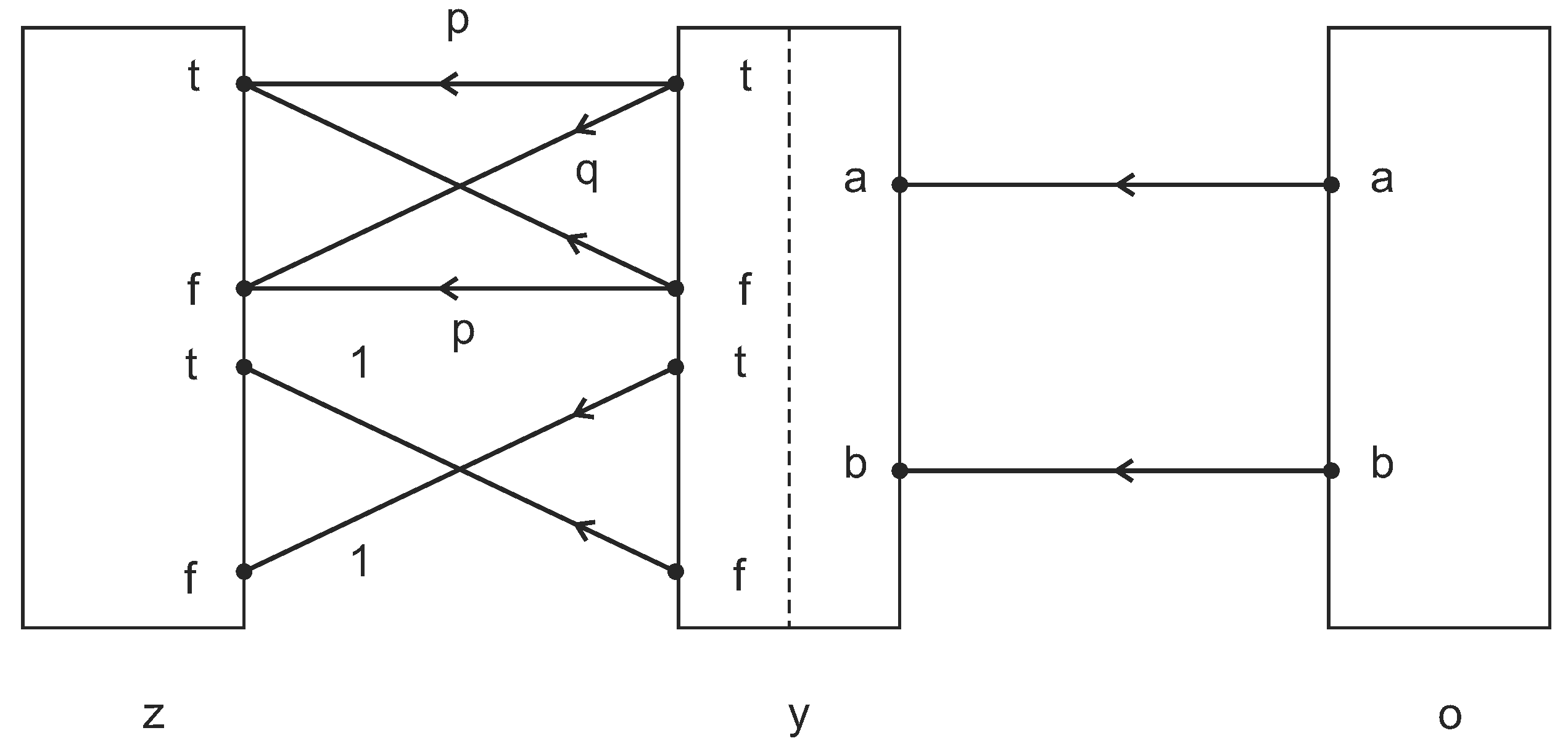
The protocol just described underlies a noisy symmetric channel between W and V. If ${\xi }_t=1$, this channel is characterized by δ and has a capacity of $1-H_2\left(\delta \right)$, where $H_2\left(\delta \right)$ is the Shannon entropy of a Bernoulli random variable with parameter δ. It induces a maximal loss of one bit of information for $\delta =\frac{1}{2}$. An illustration of the communication between the three parties patient-agent-prover is given in Figure 19.

Figure 19. Communication between W and V when $v_t\ne w_t$. The channels between W and V are symmetric. The labels above edges indicate transition probabilities. The box of V is divided into two sections representing her belief $v_t$ (left section) and the outcome of his verification ${\xi }_t$ (right section).

Figure 19. Communication between W and V when $v_t\ne w_t$. The channels between W and V are symmetric. The labels above edges indicate transition probabilities. The box of V is divided into two sections representing her belief $v_t$ (left section) and the outcome of his verification ${\xi }_t$ (right section).

7.1.3. Further Metaphors for Deformed Interactions

The agents in our picture all receive messages from the same oracle. This essentially suggests that a network of interactions is a construct quantizing the oracle knowledge. At every location within the network, only a quanta of this knowledge is used by way of interaction between a patient and an agent. Later on, we will show that although a single interaction may be limited in its capacity to prove the claim, the proof may yet emerge somewhere in the network, depending on its topology.

The triple patients-agent-oracle brings to mind some basic models of reasoning and information transfer. Perhaps a patient is an entity whose beliefs reflect both prior knowledge and observations. The patient is exposed to a genuine phenomenon, which the patient has not seen before. The phenomenon, which is the metaphor for an oracle, is beyond the comprehension of the patient, and hence, a number of observations are collected in an attempt to reach a definitive conclusion. These observations, however, may be distorted by limitations of the patient measuring apparatus or perhaps they contradict prevailing explanations and beliefs. In either cases, observations contain, or otherwise introduce, uncertainty. Observations are the metaphor for agents. What the patient tries to accomplish underlies the Bayesian inference paradigm.

Here is another metaphor. A patient is a decoder; an oracle is an information source; and an agent is an encoder who relays the encoded oracle message through a noisy communication channel. Alternatively, an agent-patient pair is a verifier, and the oracle is a prover who relays a message through a noisy communication channel. All metaphors reflect knowledge transfer subject to uncertainties.

7.2. Probabilistic Theorem Proving in Networks

The goal of this section is to prove Theorem 4, repeated below for convenience.

Theorem 7. $\mathrm{IP}\subseteq \mathrm{BraidIP}\left\{\delta ,\chi \right\}$ where:

$$I\left(c\delta \right)<\chi <\frac{1}{I(1-s\delta )},$$

(37)

with $I\left(p\right)\stackrel{\mathrm{def}}{=}-p^{-1}logp$. The growth rate of χ is $\mathcal{O}\left(\frac{1}{\delta }\right)$ as $\delta \to 0$.

Proof of Theorem 4. We explicitly construct a configuration of interactions that decide a language L in IP. This configuration, which is illustrated in Figure 20 for the case $\chi =4$, is a scaled up version of that in Figure 18. It involves $\chi +1$ verifiers W and $V^1,V^2,\dots ,V^{\chi }$ and χ interactions. The parameters of all interactions are the same and are $c,s,\delta$.

Figure 20. An interactive BraidIP theorem proving network with five verifiers W, $V^1$, $V^2$, $V^3$ and $V^4$ and four interactions.

Figure 20. An interactive BraidIP theorem proving network with five verifiers W, $V^1$, $V^2$, $V^3$ and $V^4$ and four interactions.

Let $L\in \mathrm{IP}$. The initial beliefs at time $t=0$ are set to $\left|W_0\right)\stackrel{\mathrm{def}}{=}\left|\mathrm{False}\right)$ and:

$$\left|V_0^i\right)\stackrel{\mathrm{def}}{=}\left\{\begin{array}{cc}\frac{1}{2}\left|\mathrm{False}\right)+\frac{1}{2}\left|\mathrm{True}\right),\hfill & 1<i<\chi ;\hfill \\ \left|\mathrm{True}\right),\hfill & i=\chi .\hfill \end{array}\right.$$

(38)

Thus, at time zero, there are two verifiers with opposite beliefs and $\chi -1$ verifiers whose initial belief is that the claim $x\in L$ is 50% true and 50% false.

Calculating the output statistic $\left|W_{\chi }\right)$ (which occurs at time χ) yields:

$$\left|W_{\chi }\right)⟶\left\{\begin{array}{cc}{(1-c\delta )}^{\chi }\left|\mathrm{False}\right)+\left[1-c\delta -{(1-c\delta )}^{\chi }\right]\left(\frac{1}{2}\left|\mathrm{False}\right)+\frac{1}{2}\left|\mathrm{True}\right)\right)+c\delta \left|\mathrm{True}\right),\hfill & x\in L;\hfill \\ {(1-s\delta )}^{\chi }\left|\mathrm{False}\right)+\left[1-s\delta -{(1-s\delta )}^{\chi }\right]\left(\frac{1}{2}\left|\mathrm{False}\right)+\frac{1}{2}\left|\mathrm{True}\right)\right)+s\delta \left|\mathrm{True}\right),\hfill & x\notin L.\hfill \end{array}\right.$$

(39)

From Equation (39), we see that the configuration in Figure 20 decides L if and only if:

$$\begin{array}{c}x\in L⟶{(1-c\delta )}^{\chi }<c\delta ;\hfill \\ x\notin L⟶{(1-s\delta )}^{\chi }>s\delta .\hfill \end{array}$$

(40)

From here, we obtain the following bounds for χ:

$$\frac{log\left(c\delta \right)}{log(1-c\delta )}<\chi <\frac{log\left(s\delta \right)}{log(1-s\delta )}.$$

(41)

Equation (2) follows upon noting that $log(1-p)<-p$ for any $p\in (0,1)$. Therefore:

$$-\frac{1-p}{log(1-p)}>\frac{logp}{log(1-p)}>-\frac{logp}{p}.$$

(42)

For χ within these bounds, the above configuration decides L.     ☐

Remark 9. Equation (2) tells us that χ has approximately the same growth rate in $\left|x\right|$ as $\frac{1}{\delta }$. By definition of BraidIP, χ’s growth rate is polynomial in the word length $\left|x\right|$, and so, therefore, δ is asymptotically bounded below by approximately one over a polynomial in $\left|x\right|$.

8. Efficient IP Strategies: Tangled IP

8.1. The Complexity Class TangIP

We may extend class BraidIP by allowing each verifier to have its own “local” time parameter, so that a patient belief $W_t$ may interact with an agent belief $V_s$ for $s\ne t$ and become updated to $W_{t+1}$.

(43)

We also allow verifiers to travel backwards or forwards in time and to update their previous or future beliefs, so that $V_t$ may be updated by agent $V_s$ to become $V_{t+1}$, where $V_t$ and $V_s$ are beliefs of one and the same verifier. Thus, each verifier may update their beliefs with past or future beliefs of itself (via feedback loops) or of other verifiers. We write M for a network of such concatenated interactions, subject to parameters $0<c<s\le 1$ and $\delta \in \mathbb{Q}\cap (0,1)$. An example of such a network is given in Section 8.2.

A language $L\subseteq {\{0,1\}}^{*}$ is said to be decided by M if M contains a verifier V whose belief at time χ is $\left|V_{\chi }\right)\stackrel{\mathrm{def}}{=}a\left|\mathrm{True}\right)+b\left|\mathrm{False}\right)$, such that for a fixed constant $\kappa >0$, the inequalities Equation (32) are satisfied.

The class “tangled interactive polynomial time” (TangIP) consists of those languages that are decidable for any fixed $\kappa >0$ by some network M, which contains χ interactions, where χ is polynomial in $\left|x\right|$. We denote this class $\mathrm{TangIP}\{\delta ,\chi \}$.

By Theorem 4, we know that:

$$\mathrm{IP}\subseteq \mathrm{BraidIP}\subseteq \mathrm{TangIP}.$$

We wonder about the connection between our classes BraidIP and TangIP and multi-prover IP (MIP) [27]. In particular, we wonder whether $\mathrm{MIP}\subseteq \mathrm{BraidIP}$ or $\mathrm{MIP}\subseteq \mathrm{TangIP}$, particularly if we allow different interactions to have different parameters (in this note, all interactions are required to have the same parameters, because that is all we need, but there is no obstruction to considering the more general case).

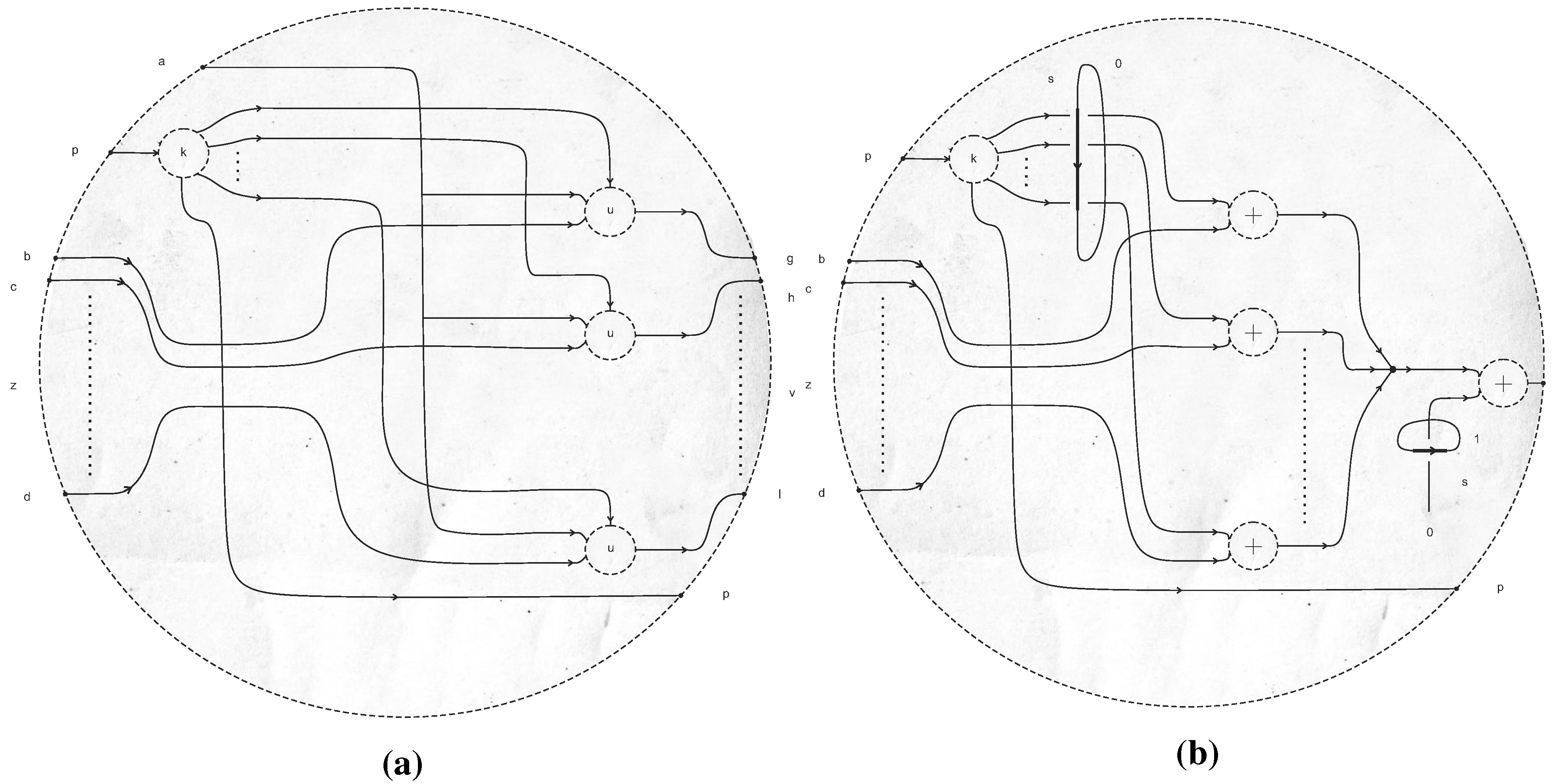
8.2. The Hopf–Chernoff Configuration

Consider an IP system whose soundness s is nearly equal to its completeness c, but for a small constant $ϵ\left(\left|x\right|\right)$ that depends on the word length $\left|x\right|$, i.e., $c-s=ϵ\left(\left|x\right|\right)$. As $ϵ\left(\left|x\right|\right)\to 0$, the IP system becomes inefficient in the sense that it accepts every word with probability nearly c regardless of its membership in L. Yet, we can still construct a deformed IP system that decides L. One may wonder how the number of interactions in such a system is affected by the decreasing gap $ϵ\left(\left|x\right|\right)$.

The number of interactions in a network of the form given in Figure 20 is implicit in Theorem 4. Fix $\delta \in \mathbb{Q}\cap (0,1)$, and note from Equation (2) that, as $ϵ\left(\left|x\right|\right)$ decreases, the values bounding χ become nearly identical. However, χ is an integer, so the two bounds must have an integer between them. In general, that means that the distance between them is at least one. Therefore, the number of interactions grows as $ϵ\left(\left|x\right|\right)$ decreases. We may need to take $\delta \to 0$ as $ϵ\left(\left|x\right|\right)\to 0$. In fact, it can be shown that in this case $\delta \left(\left|x\right|\right)=\mathcal{O}\left(ϵ\left(\left|x\right|\right)\right)$, which means that we require $\chi =\mathcal{O}(1/ϵ\left(\left|x\right|\right))$ interactions.

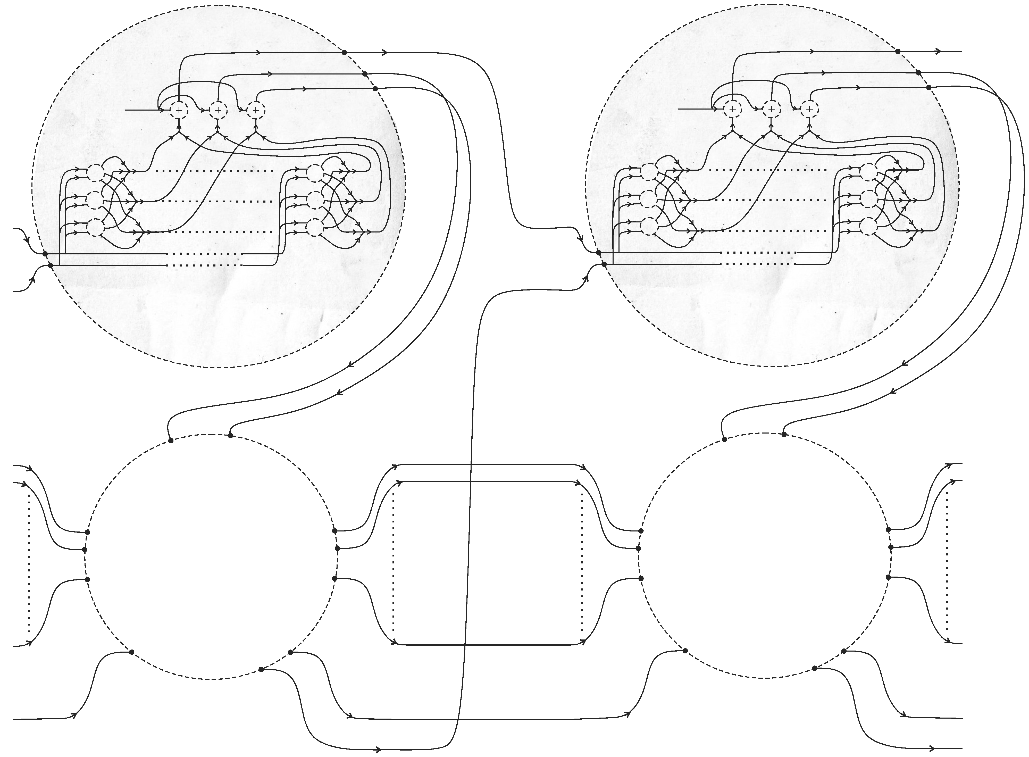
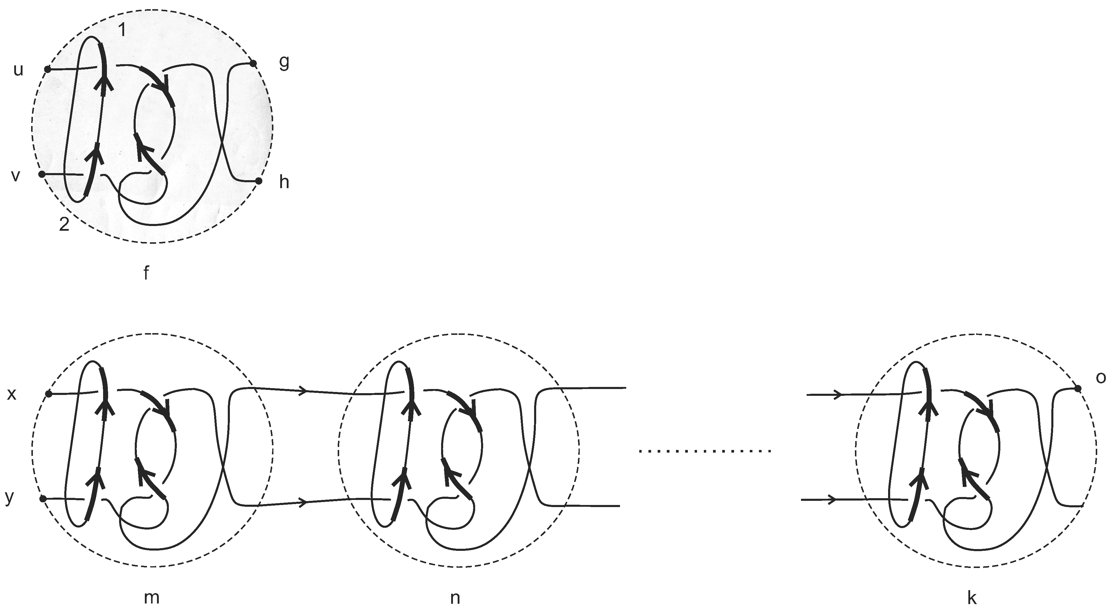
Can fewer interactions decide L ? The configuration in Figure 21 decides L for any $ϵ\left(\left|x\right|\right)$ using substantially less than $\mathcal{O}(1/ϵ\left(\left|x\right|\right))$ interactions. This machine is a concatenation of a number of identical smaller configurations of interactions, denoted $M_0,M_1,M_2,\dots$. When concatenated to form a single configuration, we require approximately $\chi =\mathcal{O}(log(1/ϵ\left(\left|x\right|\right)))$ copies of $M_0$ to decide L (the precise argument is given below). If we were to trace its colors (probability-generating functions), we would notice that it behaves much like a repetition of a binary random experiment (e.g., coin flipping), hence the magnitude of χ. We have named this configuration the Hopf–Chernoff configuration, suggesting both its structure and, to some extent, its functionality.

Figure 21. Hopf–Chernoff configuration (open version).

Figure 21. Hopf–Chernoff configuration (open version).

Theorem 8 (Hopf–Chernoff configuration). Consider the configuration of interactions in Figure 21, which underlies a deformed IP system with completeness $c\delta$ and soundness $(c-ϵ)\delta$, where $ϵ>0$. There exists a pair of beliefs, α and β, independent of any other belief in the machine, such that for any given set of initial beliefs ${\mathrm{In}}_j^0$, the machine decides any $L\in \mathrm{IP}$ using $\chi =\mathcal{O}(log(1/ϵ\left)\right)$ sub-machines (and $4\chi$ interactions). In particular, letting:

$$\begin{array}{l}\left|\alpha \right)=\left(\frac{1}{4}+\frac{1}{12}ϵ\delta \right)\left|\mathrm{True}\right)+\left(\frac{3}{4}-\frac{1}{12}ϵ\delta \right)\left|\mathrm{False}\right);\\ \left|\beta \right)=\left(1-\frac{1}{2}c\delta +\frac{1}{12}ϵ\delta \right)\left|\mathrm{True}\right)+\left(\frac{1}{2}c\delta -\frac{1}{12}ϵ\delta \right)\left|\mathrm{False}\right).\end{array}$$

(44)

yields:

$${\mathrm{Out}}_1^{\chi }⟶\left\{\begin{array}{cc}\left[\frac{1}{2}+\frac{1}{12}ϵ\delta \right]\left|\mathrm{True}\right)+\left[\frac{1}{2}-\frac{1}{12}ϵ\delta \right]\left|\mathrm{False}\right),\hfill & x\in L;\hfill \\ \left[\frac{1}{2}-\frac{1}{12}ϵ\delta \right]\left|\mathrm{True}\right)+\left[\frac{1}{2}+\frac{1}{12}ϵ\delta \right]\left|\mathrm{False}\right),\hfill & x\notin L.\hfill \end{array}\right.$$

(45)

namely, ${\mathrm{Out}}_1^{\chi }=\left[\frac{1}{2}+\frac{1}{12}ϵ\delta \right]\left|\mathrm{True}\right)+\left[\frac{1}{2}+\frac{1}{12}ϵ\delta \right]\left|\mathrm{False}\right)$.

Proof. Let us begin by writing down the relations between the outputs ${\mathrm{Out}}_j$ and inputs ${\mathrm{In}}_j$ of this machine. Note that:

$${\mathrm{Out}}_1={\left({\mathrm{In}}_1^{\left|\alpha \right)}\right)}^{\left({\mathrm{In}}_2^{\left|\beta \right)}\right)},{\mathrm{Out}}_2={\left({\mathrm{In}}_2^{\left|\beta \right)}\right)}^{\left({\mathrm{In}}_1^{\left|\alpha \right)}\right)}.$$

(46)

Explicitly writing Equation (46) using the formal parameter h yields:

$$\left[\begin{array}{c}{\mathrm{Out}}_1^i\\ {\mathrm{Out}}_2^i\end{array}\right]=\underset{\stackrel{\mathrm{def}}{=}A\left(h\right)}{\underbrace{\left[\begin{array}{cc}{(1-h)}^2& h(1-h)\\ h(1-h)& {(1-h)}^2\end{array}\right]}}\left[\begin{array}{c}{\mathrm{In}}_1^i\\ {\mathrm{In}}_2^i\end{array}\right]+\underset{\stackrel{\mathrm{def}}{=}B\left(h\right)}{\underbrace{\left[\begin{array}{cc}h(1-h)& h^2\\ h^2& h(1-h)\end{array}\right]}}\left[\begin{array}{c}\left|\alpha \right)\\ \left|\beta \right)\end{array}\right].$$

(47)

Letting ${\mathrm{In}}_j^{i+1}={\mathrm{Out}}_j^i$, $j=1,2$, Equation (47) underlies a linear dynamical system. It is easy to verify that the eigenvalues of the transition matrix $A\left(h\right)$ all are within the unit circle, i.e., $\left|\lambda \left(A\right(h\left)\right)\right|<1$ for any $h>0$. That means that the system Equation (47) reaches a steady state as $i\to \infty$. The steady state can be obtained as follows. Rewrite Equation (47) as:

$$\left[\begin{array}{c}{\mathrm{Out}}_1\\ {\mathrm{Out}}_2\end{array}\right]=A\left(h\right)\left[\begin{array}{c}{\mathrm{Out}}_1\\ {\mathrm{Out}}_2\end{array}\right]+B\left(h\right)\left[\begin{array}{c}\left|\alpha \right)\\ \left|\beta \right)\end{array}\right],$$

(48)

and solve for ${\mathrm{Out}}_1$ and ${\mathrm{Out}}_2$. Thus,

$$\left[\begin{array}{c}{\mathrm{Out}}_1\\ {\mathrm{Out}}_2\end{array}\right]={(I-A\left(h\right))}^{-1}B\left(h\right)\left[\begin{array}{c}\left|\alpha \right)\\ \left|\beta \right)\end{array}\right]=\frac{1}{3-2h}\left[\begin{array}{c}2(1-h)\left|\alpha \right)+\left|\beta \right)\\ \left|\alpha \right)+2(1-h)\left|\beta \right)\end{array}\right].$$

(49)

Define:

$$\begin{array}{c}\left|\alpha \right)\stackrel{\mathrm{def}}{=}a\left|\mathrm{True}\right)+(1-a)\left|\mathrm{False}\right);\hfill \\ \left|\beta \right)\stackrel{\mathrm{def}}{=}b\left|\mathrm{True}\right)+(1-b)\left|\mathrm{False}\right).\hfill \end{array}$$

(50)

For the network to decide L, we require the steady state of ${\mathrm{Out}}_1$ to satisfy:

$${\mathrm{Out}}_1⟶\left\{\begin{array}{cc}(\frac{1}{2}+\sigma )\left|\mathrm{True}\right)+(\frac{1}{2}-\sigma )\left|\mathrm{False}\right),\hfill & x\in L;\hfill \\ 0pt12pt(\frac{1}{2}-\sigma )\left|\mathrm{True}\right)+(\frac{1}{2}+\sigma )\left|\mathrm{False}\right),\hfill & x\notin L.\hfill \end{array}\right.$$

(51)

for some $\sigma >0$. Using both Equation (49) and Equation (50), this requirement translates into the following set of equations:

$$\begin{array}{cc}(3-2c\delta )\left(\frac{1}{2}+\sigma \right)=2(1-c\delta )a+b,\hfill & x\in L;\hfill \\ (3-2(c-ϵ)\delta )\left(\frac{1}{2}-\sigma \right)=2(1-(c-ϵ)\delta )a+b,\hfill & x\notin L.\hfill \end{array}$$

(52)

where the fact that $h=c\delta$ for $x\in L$ and $h=(c-ϵ)\delta$ for $x\notin L$ has been used. Solving Equation (52) for the coefficients a and b while assuming $\sigma =\frac{1}{12}ϵ\delta$ yields Equation (44). The underlying output probabilities in Equation (45) are given by Equation (51).

To complete the argument, we need to show that the network converges within the stated number of iterations. It is sufficient to consider the case where the output probabilities Equation (51) is attained to within the order $\mathcal{O}\left(\sigma \right)=\mathcal{O}\left(ϵ\right)$. The growth rate of the system Equation (47) is linear in ${\left|{\lambda }_1\left(A\left(h\right)\right)\right|}^{\chi }$ where ${\lambda }_1\left(A\left(h\right)\right)$ denotes the largest eigenvalue of $A\left(h\right)$. Simple calculation shows that ${\lambda }_1\left(A\left(h\right)\right)=1-h$, which yields $\chi =\mathcal{O}(log(1/ϵ\left)\right)$.     ☐

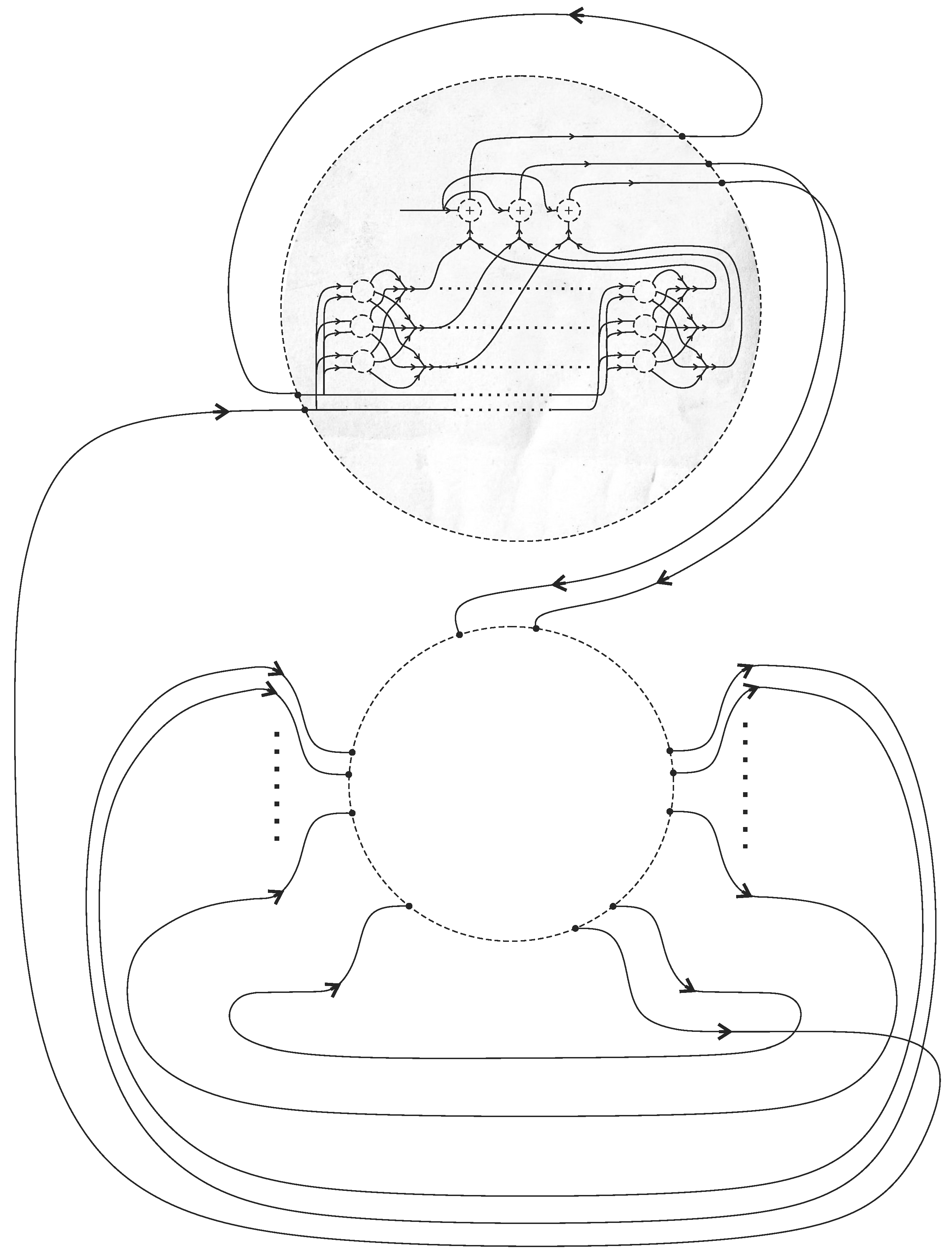
The Hopf–Chernoff configuration is a recursive structure, which is guaranteed to converge irrespective of its initial beliefs ${\mathrm{In}}_j^0$. In fact, it represents a two-dimensional homogeneous irreducible Markov chain whose rate of convergence is $\mathcal{O}\left(2^{-\chi }\right)$. Its stationary distribution, which depends on whether $x\in L$ or $x\notin L$, is given by Equation (45). By virtue of its convergence properties, we may just let it run forever (i.e., $\chi \to \infty$) knowing that it will eventually reach a stationary distribution not far from Equation (45). For that reason, we may as well substitute the open network in Figure 21 with its closed counterpart in Figure 22.

Figure 22. Hopf–Chernoff configuration (closed version).

Figure 22. Hopf–Chernoff configuration (closed version).

9. PCP Networks

In this section, we specialize to non-adaptive three-bit verifiers, to exhibit that tangle machines may exhibit better performance parameters than classical systems.

We deform the Håstad PCP verifier, which has $c=1$ and $s\approx 0.75$. Suppose the two verifiers disagree, $v_t\ne w_t$, where $v_t,w_t\in \{\left|\mathrm{True}\right),\left|\mathrm{False}\right)\}$. In this case, the interaction proceeds as follows. The patient verifier W provides the addresses of three bits to Π. These bits are received by the agent verifier V, which computes a certificate ${\xi }_t$, which is equal either to one, meaning “accept”, or to $-1$, meaning “reject”. The agent then flips one out of the three bits with the following probabilities:

• $({\xi }_t=1)$∧$(v_t=\left|\mathrm{True}\right))$⟶V flips a bit with probability $1-\delta$.
• $({\xi }_t=1)$∧$(v_t=\left|\mathrm{False}\right))$⟶V flips a bit with probability δ.
• $({\xi }_t=-1)$∧$(v_t=\left|\mathrm{True}\right))$ ⟶ V flips no bit.
• $({\xi }_t=-1)$∧$(v_t=\left|\mathrm{False}\right))$ ⟶ V flips a bit.

The corrupted set of bits is then sent back to W, who computes her own certificate. This protocol realizes the communication channel in Figure 19.

9.1. A Better Than Classical PCP Verifier

In this section, we construct a tangle machine whose interactions are deformed Håstad verifiers, which has perfect accuracy and a completeness of $\frac{2}{3}+\sigma \approx 0.667$. This is worse than the conjectured bound of $0.625$, but better than the best-known classical non-adaptive three-bit PCP protocol, whose soundness is only around $0.741$. Thus, our machine behaves like a single very good verifier.

Our machine makes use of the Hopf–Chernoff configuration in Figure 21.

• Choose input beliefs ${\mathrm{In}}_j^0$, $j=1,2$, arbitrarily from $\{\left|\mathrm{True}\right),\left|\mathrm{False}\right)\}$. Assume $c=1$, and fix δ.
• Let α be a Bernoulli distribution with parameter $\frac{1}{2}$. Draw a belief from α for the top agent, and set the bottom agent to the negation of that belief. We color the bottom agent as $\neg \alpha$, which equals α as a distribution, to diagrammatically signify what we are doing.
• Do the following for $i=1,\dots ,\chi$, where $\chi =\mathcal{O}\left(1\right)$:

  • Using the underlying deformed PCP verifier, perform the four interactions of the Hopf–Chernoff configuration to propagate the beliefs of the two verifiers from ${\mathrm{In}}_j^i$ to ${\mathrm{Out}}_j^i$ according to the diagram below.
  • Set ${\mathrm{In}}_j^i={\mathrm{Out}}_j^{i-1}$, $j=1,2$.
• If the patient belief in the output ${\mathrm{Out}}_1^{\chi }=\neg \alpha$, then return $\left|\mathrm{True}\right)$; otherwise, return $\left|\mathrm{False}\right)$.

Theorem 9. The Hopf–Chernoff machine approaches perfect completeness and soundness at most $\frac{1}{3-2s}$ as $\delta \to 1.$ In particular, if we put deformed Håstad verifiers at interactions, its soundness is at most $\frac{2}{3}$.

Proof.

• Completeness Assume that $x\in L$, and note that as $\delta \to 1$, so does $h=c\delta \to 1$. In the limit where $h=1$, note that by Equation (41), the Hopf–Chernoff swaps the beliefs α and $\neg \alpha$, such that always ${\mathrm{Out}}_1=\neg \alpha$ and ${\mathrm{Out}}_2=\alpha$. Thus, Step (iv) of the algorithm concludes with $\left|\mathrm{True}\right)$.
• Soundness The soundness of the algorithm bounds the probability that ${\mathrm{Out}}_1=\neg \alpha$ in the case where $x\notin L$. This probability is given by:

  $$\begin{array}{ll}Pr({\mathrm{Out}}_1=\neg \alpha )=Pr({\mathrm{Out}}_1=& \left|\mathrm{True}\right)\mid \alpha =\left|\mathrm{False}\right))Pr(\alpha =\left|\mathrm{False}\right))\\ & \hspace{1em}\hspace{1em}+Pr({\mathrm{Out}}_1=\left|\mathrm{False}\right)\mid \alpha =\left|\mathrm{True}\right))Pr(\alpha =\left|\mathrm{True}\right)).\end{array}$$

  (53)
  Although not truly essential, the algorithm assumes $Pr(\alpha =\left|\mathrm{True}\right))=\frac{1}{2}$. The conditional probabilities above can be bounded using Equation (41) as follows. Take $h=s\delta \to s$ and assume that $\left|\alpha \right)=\left|\mathrm{False}\right)$. In this case, Equation (41) implies:

  $$Pr({\mathrm{Out}}_1=\left|\mathrm{True}\right)\mid \alpha =\left|\mathrm{False}\right))\le \frac{1}{3-2s}.$$

  (54)
  On the other hand, letting $\left|\alpha \right)=\left|\mathrm{True}\right)$, the same equation reads:

  $$Pr({\mathrm{Out}}_1=\left|\mathrm{False}\right)\mid \alpha =\left|\mathrm{True}\right))\le \frac{1}{3-2s}.$$

  (55)
  This follows from the fact that the algorithm decides $x\in L$ if ${\mathrm{Out}}_1=\neg \alpha$ irrespective of the beliefs themselves. For that reason, these equations coincide, though for different values of α and ${\mathrm{Out}}_1$. Both describe a failure of the algorithm to decide $x\notin L$. The theorem now follows from Equation (53)–(55).

☐

10. Low-Dimensional Topology and Bisimulation

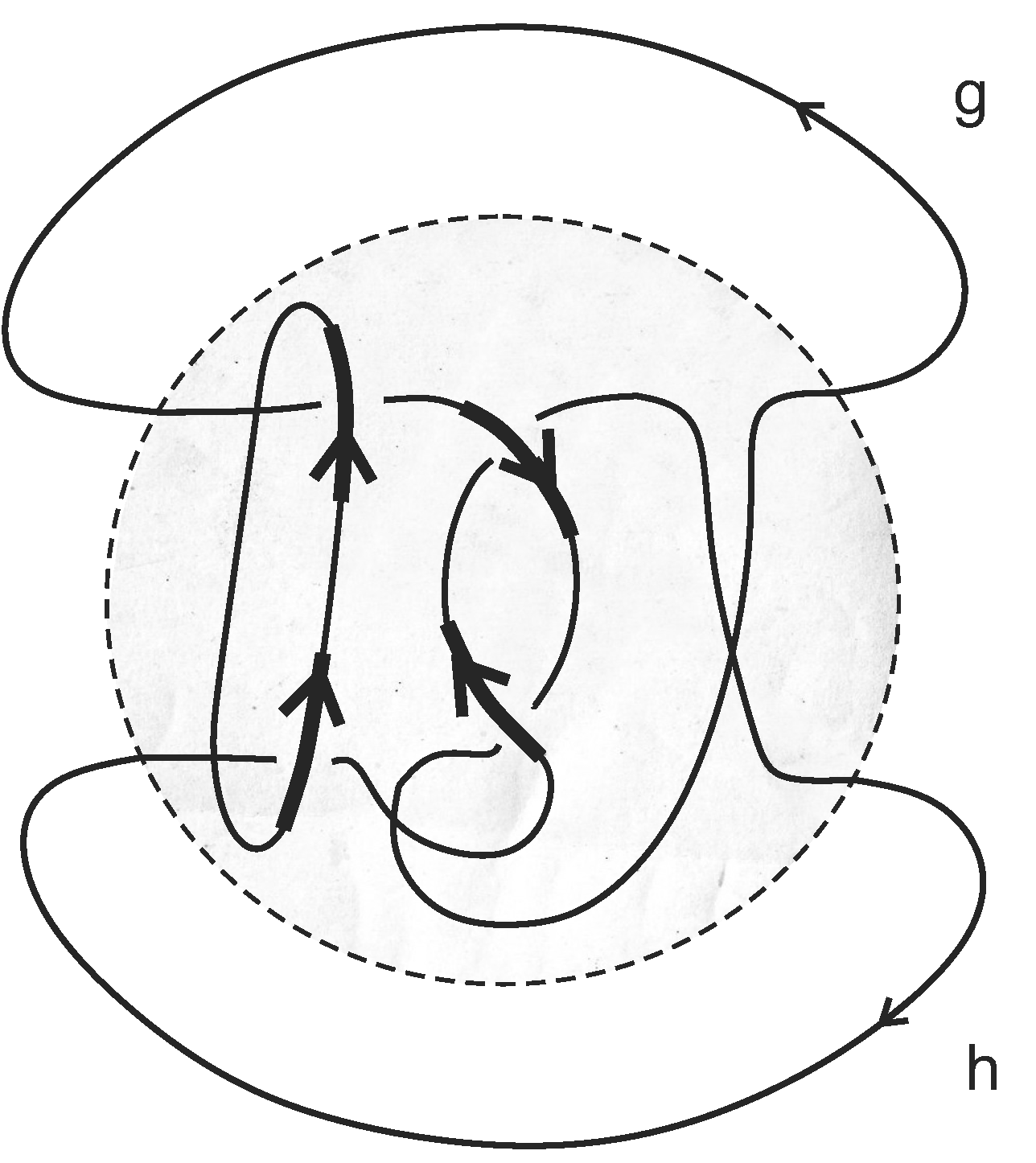
Definition 10. Tangle machines M and $M^{\prime }$, which each come equipped with a distinguished set of input and output registers, are bisimilar if any computation that can be carried out on M can be carried out on $M^{\prime }$ and vice versa.

Because computations are defined only with respect to the pre-chosen sets of input and of output registers, Definition 10 encapsulates what may be thought of as a weak notion of bisimulation (no requirement is made on “silent” or “internal” interactions).

In Section 10.1, we formulate a set of local moves, such that any two machines related by these local moves are bisimilar. In Section 10.2, we discuss a feature of our formalism, that is the “unsplittability” of our agent registers. In Section 10.3, we suggest an application of machine equivalence to define a notion of zero knowledge for tangle machines and to utilize it to construct TangIP machines, which are “more secure” in a specific sense. We give an example in Section 10.4. Finally, in Section 10.5, we extend our notion of machine equivalence to machines that may have wyes.

10.1. Equivalence

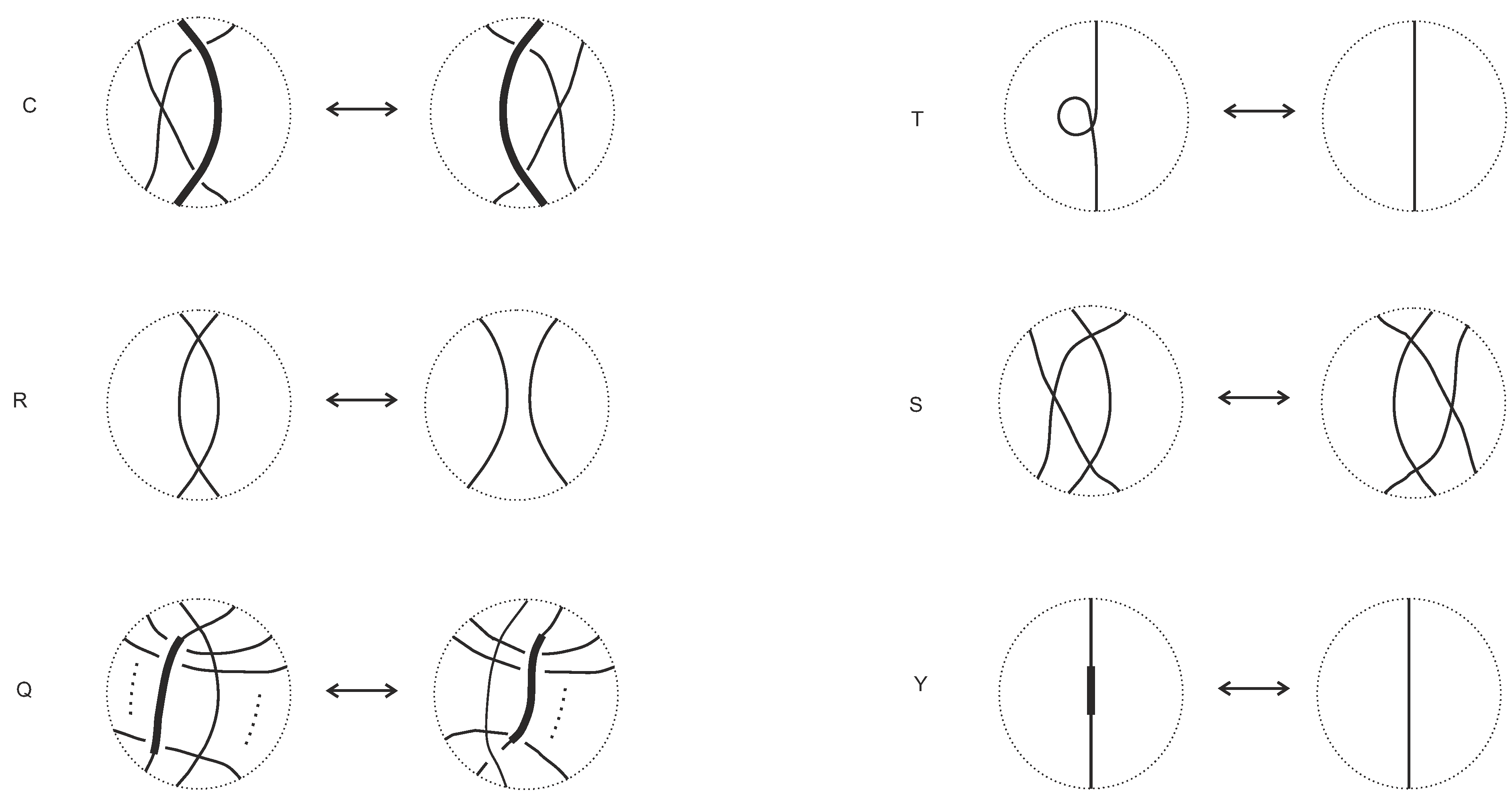
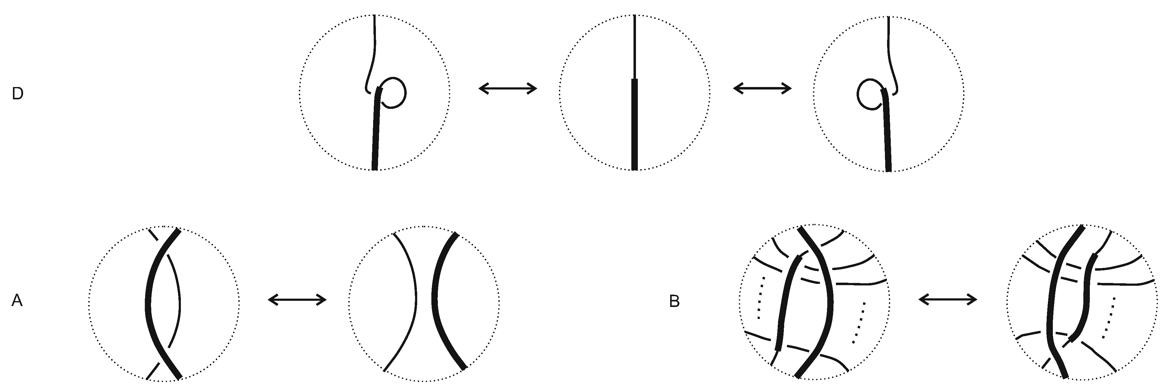
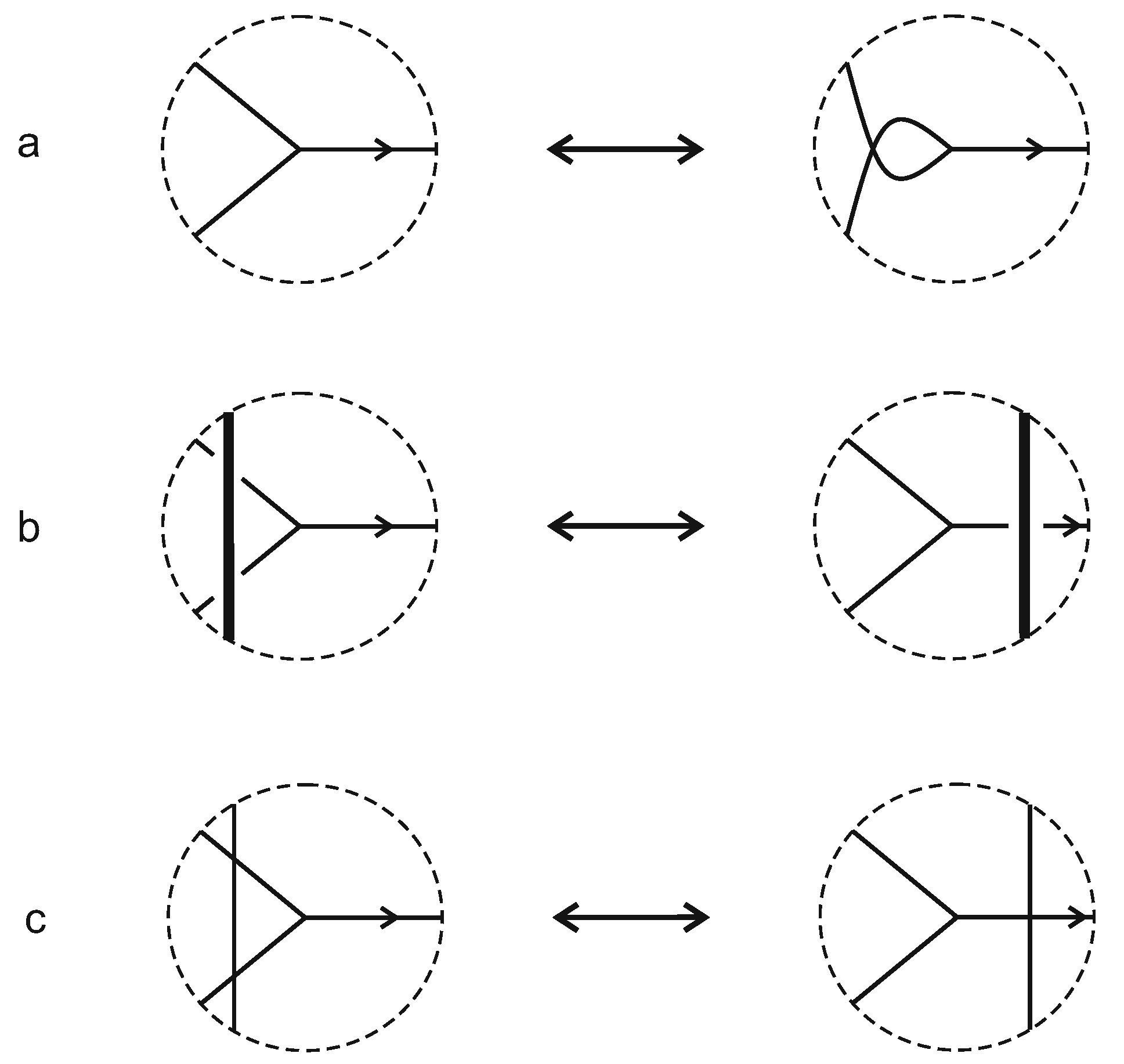
The key property of tangle machines is that they admit a local notion of equivalence [1]. Two (quandle colored, without wyes) tangle machines are equivalent if they are related by a finite sequence of the moves in Figure 23 and Figure 24. It is forbidden for these moves to involve input and output registers of a computation.

Figure 23. Cosmetic moves for machines. Directions are not indicated, meaning that the moves are valid for any direction and the same for colorings.

Figure 23. Cosmetic moves for machines. Directions are not indicated, meaning that the moves are valid for any direction and the same for colorings.

Figure 24. Reidemeister moves for machines, valid for any directions of the agents. It is forbidden for these moves to involve input and output registers of a computation.

Figure 24. Reidemeister moves for machines, valid for any directions of the agents. It is forbidden for these moves to involve input and output registers of a computation.

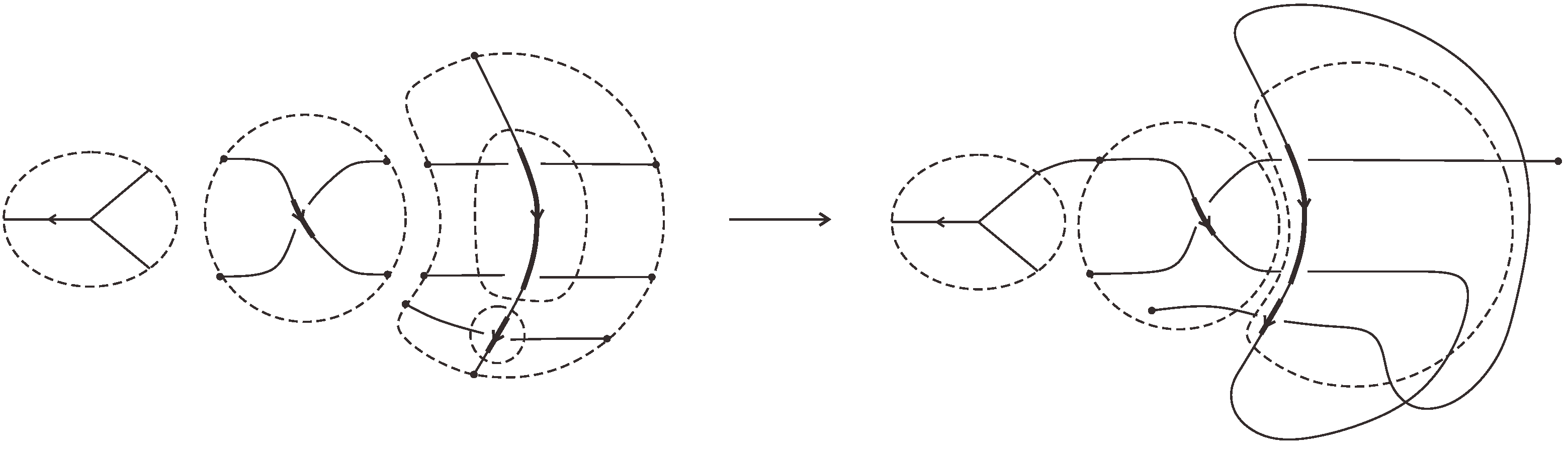
Two machines related by the local moves in Figure 23 carry out identical computations, and it follows from the construction of an interaction that two machines related by $\mathrm{R}1$ differ only by a trivial computation at which “nothing happens”. Thus, the interesting moves for us are $\mathrm{R}2$ and $\mathrm{R}3$ in Figure 24, about which we will say more later.

Remark 10. First note that, for $\mathrm{R}2$ to make sense, all participating colors must be defined. This requirement is non-trivial for a machine colored by a quandloid.

Remark 11. For a machine colored by a quagma, the $\mathrm{R}3$ move is replaced by the following:

(56)

for all $▹,▸\in B$ satisfying $(x▹y)▸z=(x▸z)▹(y▸z)$ for all $x,y,z\in Q$.

If we choose input and output registers to be machine endpoints, then equivalent machines have identical initial and terminal beliefs, which implies that both machines have the same computational power in terms of deciding a language. Nevertheless, the local behavior of equivalence may be different, in that the colors of intermediate interactions in between the same initial and terminal statistics may be different in equivalent machines. As in the earlier example in Figure 18, equivalent machines may have two different prover strategies arriving at the same proof.

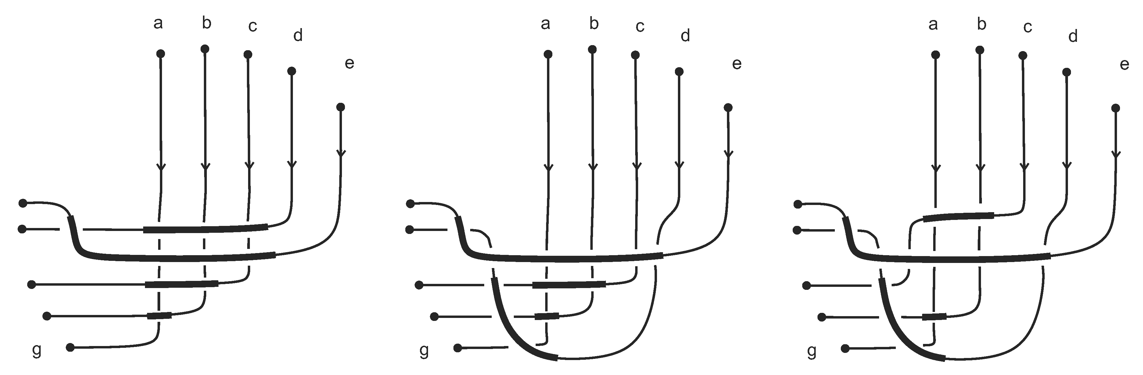
To expand that example, Figure 25 features several equivalent prover strategies for the machine in Figure 20, all of which are obtained by application of $\mathrm{R}3$ moves.

Figure 25. Equivalent prover strategies for the machine in Figure 20.

Figure 25. Equivalent prover strategies for the machine in Figure 20.

10.2. The Single Agent in R2 and R3

In this section, we discuss the single agent that acts on numerous patients and cannot be split. Such an agent features in Moves $\mathrm{R}2$ and $\mathrm{R}3$ and distinguishes our approach, e.g., from w-tangles [35].

The $\mathrm{R}2$ move tells us that computations are reversible, in the sense that any operation $▹\in B$ has an inverse operation $◃\in B$, such that no information is computed from $(x▹y)◃y$ for any $x,y\in Q$. Because we are working not only with colors, but with realizations of belief statistics, we are saying more than just $(x▹y)◃y=x$. We require that there be zero knowledge gain about realizations of $(x▹y)◃y$ from a realization of x.

(57)

Our formalism features agents that act on multiple patients. These actions are independent by definition. Conversely, as we saw in Section 8.2, different agents may cooperate, for example, by coordinating their realizations to be the same or to be opposed to one another.

We do not impose the following a priori reasonable generalization of $\mathrm{R}2$.

(58)

One reason that we do not impose Equation (58) can be seen by considering the example in which the two agents in the machine on the left-hand side adopt the strategy of always offering the same realization. If the realization of the patient and of the agent coincide, we can compute the realizations of both other patients. If not, then we cannot. Thus, we can compute the colors of the remaining patients in Equation (58) for some realizations, but not for others. This behavior is not shared by the machine on the right-hand side, in which colors of the realizations of patients can never be computed unless they are already given. If the choice of realization is independent for both patients, i.e., if there is only a single interaction, as in the case of “honest” $\mathrm{R}2$, there is no such phenomenon, and no choice of realizations for input registers is distinguished from any other. Note also that Equation (58) represents two distinct computations, each of which can be considered separately and each of which is non-trivial, which is not true for the right-hand side of the “honest” $\mathrm{R}2$.

For the same reason, we do not impose the following “fake $\mathrm{R}3$ move”:

(59)

10.3. Zero Knowledge

The theory of IP features the notion of a zero-knowledge proof [26,48]. In a zero-knowledge proof, the information that may be gained by the verifier in the course of her interactions with the prover are restricted. This is useful when the verifier may not always be trustworthy. The definition makes use of a simulator, which is an arbitrary feasible algorithm that is able to reproduce the transcript of such an interaction without ever interacting with the prover.

We suggest the following definition as a TangIP analogue to the notion of zero knowledge.

Definition 11 (Zero-knowledge tangle machine). A tangle machine M that decides a language $L\in \mathrm{TangIP}$ is said to be zero knowledge if the following is satisfied.

1.

There are no intermediate interactions in M that decide L.

2.

There exists an equivalent machine $M^{\prime }$, which decides L at one of its intermediate interactions.

Remark 12. The idea of zero-knowledge tangled IP parallels the authors’ model of fault-tolerant information fusion networks, except that there, we wanted intermediate registers to “know as much as possible”, whereas here, we want them to “know as little as possible” [4].

As a generic example, consider machines $M^{\prime }$ and M in Figure 26. Both share the same initial and terminal belief statistics. The explicit structure of the machines is mostly irrelevant, except that they both contain a sub-machine S, which we graphically represent by a blank disk, with the property that M, $M^{\prime }$, and some of S’s terminal statistics $\left|Y_i\right)$ decide L. In M, the verifier Z is an agent to all initial states of S, and the resulting beliefs from this interaction are $\left|X_i\right)$, $i=1,2,\dots$ In $M^{\prime }$, the same verifier is an agent to the terminal states of S, and the resulting beliefs from this interaction are characterized by $\left|Y_i\right)$.

Figure 26. Two equivalent machines. The machine M is zero knowledge. The proper sub-machine S determines L.

Figure 26. Two equivalent machines. The machine M is zero knowledge. The proper sub-machine S determines L.

That M is zero knowledge implies that the proof should not appear somewhere within it. Assuming none of the ${\mathrm{In}}^{\prime }s$ decide L and neither do any intermediate belief states of S, this requirement implies that none of the $\left|X_i\right)={\left({\mathrm{In}}_i\right)}^{\left|Z\right)}$ decide L. On the other hand, the machine $M^{\prime }$ shows us that an interaction between the terminal states of S, some of which decide L, with the agent Z are able to produce the proof. That is, some of ${\mathrm{Out}}_i={\left|Y_i\right)}^{\left|Z\right)}$ decide L. These requirements completely characterize the belief distribution $\left|Z\right)$. Perhaps unsurprisingly, it turns out that $\left|Z\right)=\frac{1}{2}\left|\mathrm{True}\right)+\frac{1}{2}\left|\mathrm{False}\right)$.

Ideally, we would require that S reproduces the proof as if it were produced by M itself. This requirement translates into:

$$\left|Y_i\right)={\mathrm{Out}}_i,$$

(60)

for any ${\mathrm{Out}}_i$ that decides L. As both sides of Equation (60) depend on the deformation parameter δ, this equation may be used to determine δ, such that M is zero knowledge. Below, we give an example.

10.4. Example

Consider the two machines in Figure 27. Assume they both employ a deformed IP system whose completeness and soundness are δ and $\frac{1}{2}\delta$. Let $\left|Z\right)=\frac{1}{2}\left|\mathrm{False}\right)+\frac{1}{2}\left|\mathrm{True}\right)$, and let us first see what the value of δ is for the machine to decide L. The output $\left|X_2\right)$ of either machines is given by:

$$\left|X_2\right)⟶\left\{\begin{array}{cc}\left[{(1-\delta )}^2+\frac{1}{2}\delta \right]\left|\mathrm{False}\right)+\left[\delta (1-\delta )+\frac{1}{2}\delta \right]\left|\mathrm{True}\right),\hfill & x\in L;\hfill \\ \left[{(1-\frac{1}{2}\delta )}^2+\frac{1}{4}\delta \right]\left|\mathrm{False}\right)+\left[\frac{1}{2}\delta (1-\frac{1}{2}\delta )+\frac{1}{4}\delta \right]\left|\mathrm{True}\right),\hfill & x\notin L.\hfill \end{array}\right.$$

(61)

from which we conclude that $\delta >\frac{1}{2}$. The machine on the right in this figure is zero knowledge, because $\left|X_1\right)$ does not decide L:

$$\left|X_1\right)⟶\left\{\begin{array}{cc}\left[1-\frac{1}{2}\delta \right]\left|\mathrm{False}\right)+\frac{1}{2}\delta \left|\mathrm{True}\right),\hfill & x\in L;\hfill \\ \left[1-\frac{1}{4}\delta \right]\left|\mathrm{False}\right)+\frac{1}{4}\delta \left|\mathrm{True}\right),\hfill & x\notin L.\hfill \end{array}\right.$$

(62)

and on the other hand, the sub-machine inside the small disk on the left decides L:

$$\left|{\overline{X}}_1\right)⟶\left\{\begin{array}{cc}\left[1-\delta \right]\left|\mathrm{False}\right)+\delta \left|\mathrm{True}\right),\hfill & x\in L;\hfill \\ \left[1-\frac{1}{2}\delta \right]\left|\mathrm{False}\right)+\frac{1}{2}\delta \left|\mathrm{True}\right),\hfill & x\notin L.\hfill \end{array}\right.$$

(63)

Figure 27. Example of a zero-knowledge machine.

Figure 27. Example of a zero-knowledge machine.

If we further restrict the value of δ so as to satisfy Equation (60), namely,

$$\left|{\overline{X}}_1\right)={\left|X\right)}_2⟶\delta =\delta (1-\delta )+\frac{1}{2}\delta ,$$

(64)

we obtain $\delta =\frac{1}{2}$, which obviously contradicts the basic requirement of deciding L. If we slightly relax this condition to allow a small discrepancy between the underlying distributions, then we may take $\delta =\frac{1}{2}+\kappa \left(x\right)$, where $\kappa \left(x\right)$ is a statistical distance, which potentially depends on x.

10.5. Equivalence for Machines with Wyes

Machines colored by quagmas as machines with wyes also have a notion of equivalence, giving them a certain flexibility as a diagrammatic language. Two trivalent machines are equivalent if they are related by a finite sequence of moves in Figure 23, Figure 24 and Figure 28.

Figure 28. Local moves for wyes. Note that $\mathrm{YR}3$ may reverse the label on the wye (max to min or vice versa), depending on what the colors are.

Figure 28. Local moves for wyes. Note that $\mathrm{YR}3$ may reverse the label on the wye (max to min or vice versa), depending on what the colors are.

11. Conclusions

In this paper, we have suggested a Turing-complete diagrammatic model of computation, in which computers are drawn as tangles of decorated colored strings. With bounded resources, our “tangle machines” can decide any language in complexity IP, sometimes more efficiently than known classical single-verifier models. Our machines admit a notion of equivalence that they inherit from low-dimensional topology, with equivalent machines representing bisimilar computations. Topological invariants of our machines would be characteristic quantities for these computations, which are invariant over bisimilarity classes.

References

- Carmi, A.Y.; Moskovich, D. Tangle machines. Proc. R. Soc. A 2015, 471. [Google Scholar] [CrossRef]
- Churchill, F.B. William Johannsen and the genotype concept. J. Hist. Biol. 1974, 7, 5–30. [Google Scholar] [CrossRef] [PubMed]
- Johannsen, W. The genotype conception of heredity. Am. Nat. 1911, 45, 129–159. [Google Scholar] [CrossRef]
- Carmi, A.Y.; Moskovich, D. Low dimensional topology of information fusion. In Proceedings of the 8th International Conference on Bio-inspired Information and Communications Technologies, Boston, MA, USA, 1–3 December 2014; pp. 251–258.
- Shamir, A. IP = PSPACE. J. ACM 1992, 39, 869–877. [Google Scholar] [CrossRef]
- Elhamdadi, M. Distributivity in Quandles and Quasigroups. In Algebra, Geometry and Mathematical Physics; Springer: Berlin/Heidelberg, Germany, 2014; pp. 325–340. [Google Scholar]
- Peirce, C.S. On the algebra of logic. Am. J. Math. 1880, 3, 15–57. [Google Scholar] [CrossRef]
- Kauffman, L.H. Knot automata. In Proceedings of the Twenty-Fourth International Symposium on Multiple-Valued Logic, Boston, MA, USA, 25–27 May 1994; pp. 328–333.
- Kauffman, L.H. Knot logic. In Knots and Applications; Series of Knots and Everything 6; Kauffman, L., Ed.; World Scientific Publications: Singapore, 1995; pp. 1–110. [Google Scholar]
- Buliga, M.; Kauffman, L. GLC actors, artificial chemical connectomes, topological issues and knots. In Proceedings of the Fourteenth International Conference on the Synthesis and Simulation of Living Systems, New York, NY, USA, 30 July–2 August 2013; pp. 490–497.
- Meredith, L.G.; Snyder, D.F. Knots as processes: A new kind of invariant. 2010. Available online: http://arxiv.org/abs/1009.2107 (accessed on 17 July 2015).
- Kauffman, L.H.; Lomonaco, S.J., Jr. Braiding operators are universal quantum gates. New J. Phys. 2004, 6. [Google Scholar] [CrossRef]
- Nayak, C.; Simon, S.H.; Stern, A.; Freedman, M.; Sarma, S.D. Non-Abelian anyons and topological quantum computation. Rev. Mod. Phys. 2008, 80, 1083–1159. [Google Scholar] [CrossRef]
- Ogburn, R.W.; Preskill, J. Topological quantum computation. In Quantum Computing and Quantum Communications; Springer: Berlin, Germany, 1999; Volume 1509, pp. 341–356. [Google Scholar]
- Kitaev, A.Y. Fault-tolerant quantum computation by anyons. Ann. Phys. 2003, 303, 2–30. [Google Scholar] [CrossRef]
- Mochon, C. Anyons from nonsolvable finite groups are sufficient for universal quantum computation. Phys. Rev. A 2003, 67. [Google Scholar] [CrossRef]
- Alagic, G.; Jeffery, S.; Jordan, S. Circuit Obfuscation Using Braids. In Proceedings of the 9th Conference on the Theory of Quantum Computation, Communication and Cryptography, Singapore, 21–23 May 2014; Volume 27, pp. 141–160.
- Buliga, M. Computing with space: A tangle formalism for chora and difference. 2011. Available online: http://arxiv.org/abs/1103.6007 (accessed on 17 July 2015).
- Abramsky, S.; Coecke, B. Categorical quantum mechanics. In Handbook of Quantum Logic and Quantum Structures; Elsevier: Amsterdam, The Netherlands, 2009; Volume 2, pp. 261–323. [Google Scholar]
- Baez, J.; Stay, M. Physics, topology, logic and computation: A Rosetta stone. Lect. Notes Phys. 2011, 813, 95–172. [Google Scholar]
- Vicary, J. Higher Semantics for Quantum Protocols. In Proceedings of the 27th Annual ACM/IEEE Symposium on Logic in Computer Science, Los Alamitos, CA, USA, 25–28 June 2012; pp. 606–615.
- Roscoe, A.W. Consistency in distributed databases. In Oxford University Computing Laboratory Technical Monograph; Oxford University Press: Oxford, UK, 1990; Volume PRG-87. [Google Scholar]
- Turing, A.M. On computable numbers, with an application to the Entscheidungsproblem. P. Lond. Math. Soc. Ser. 2 1937, 42, 230–265. [Google Scholar] [CrossRef]
- Turing, A.M. On computable numbers, with an application to the Entscheidungsproblem: A correction. P. Lond. Math. Soc. Ser. 2 1938, 43, 544–546. [Google Scholar] [CrossRef]
- Hopcroft, J.E.; Motwani, R.; Ullman, J.D. Introduction to Automata Theory, Languages, and Computation, 2nd ed.; Addison-Wesley: Reading, MA, USA, 2001. [Google Scholar]
- Goldwasser, S.; Micali, S.; Rackoff, C. The Knowledge complexity of interactive proof-systems. SIAM J. Comput. 1989, 18, 186–208. [Google Scholar] [CrossRef]
- Ben-Or, M.; Goldwasser, S.; Kilian, J.; Wigderson, A. Multi prover interactive proofs: How to remove intractability assumptions. In Proceedings of the 20th ACM Symposium on Theory of Computing, Chicago, IL, USA, 2–4 May 1988; pp. 113–121.
- Babai, L.; Fortnow, L.; Lund, C. Non-deterministic exponential time has two-prover interactive protocols. Comput. Complex. 1991, 1, 3–40. [Google Scholar] [CrossRef]
- Arora, S.; Safra, S. Probabilistic checking of proofs: A new characterization of NP. J. ACM 1998, 45, 70–122. [Google Scholar] [CrossRef]
- Moshkovitz, D.; Raz, R. Two-query PCP with subconstant error. J. ACM 2010, 57. [Google Scholar] [CrossRef]
- Arora, S.; Lund, C.; Motwani, R.; Sudan, M.; Szegedy, M. Proof verification and hardness of approximation problems. J. ACM 1998, 45, 501–555. [Google Scholar] [CrossRef]
- Håstad, J. Some optimal inapproximability results. J. ACM 1997, 48, 798–859. [Google Scholar] [CrossRef]
- Khot, S.; Saket, R. A 3-query non-adaptive PCP with perfect completeness. In Proceedings of the 21st IEEE Conference on Computational Complexity, Prague, Czech Republic, 16–20 July 2006; pp. 159–169.
- Zwick, U. Approximation algorithms for constraint satisfaction problems involving at most three variables per constraint. In Proceedings of the 9th ACM-SIAM Symposium on Discrete Algorithms, San Francisco, CA, USA, 25–27 January 1998; pp. 201–210.
- Bar-Natan, D.; Dancso, S. Finite type invariants of w-knotted objects I: W-knots and the Alexander polynomial. 2014. Available online: http://arxiv.org/abs/1405.1956 (accessed on 17 July 2015).
- Kauffman, L.H. Virtual knot theory. Europ. J. Combinatorics 1999, 20, 663–690. [Google Scholar] [CrossRef]
- Clark, D.; Morrison, S.; Walker, K. Fixing the functoriality of Khovanov homology. Geom. Topol. 2009, 13, 1499–1582. [Google Scholar] [CrossRef]
- Buliga, M. Braided spaces with dilations and sub-riemannian symmetric spaces. In Geometry, Exploratory Workshop on Differential Geometry and Its Applications; Andrica, D., Moroianu, S., Eds.; Cluj Univ. Press: Cluj-Napoca, Romania, 2011; pp. 21–35. [Google Scholar]
- Ishii, A.; Iwakiri, M.; Jang, Y.; Oshiro, K. A G–family of quandles and handlebody-knots. Illinois J. Math. 2013, 57, 817–838. [Google Scholar]
- Przytycki, J.H. Distributivity versus associativity in the homology theory of algebraic structures. Demonstr. Math. 2011, 44, 823–869. [Google Scholar]
- Joyce, D. A classifying invariant of knots: The knot quandle. J. Pure Appl. Algebra 1982, 23, 37–65. [Google Scholar] [CrossRef]
- Abramsky, S. No-cloning in categorical quantum mechanics. In Semantic Techniques in Quantum Computation; Mackie, I., Gay, S., Eds.; Cambridge University Press: Cambridge, UK, 2010; pp. 1–28. [Google Scholar]
- Krohn, K.; Maurer, W.D.; Rhodes, J. Realizing complex boolean functions with simple groups. Inform. Control 1966, 9, 190–195. [Google Scholar] [CrossRef]
- Barrington, D.A. Bounded-width polynomial-size branching programs recognize exactly those languages in NC1. J. Comput. System Sci. 1989, 38, 150–164. [Google Scholar] [CrossRef]
- Fredkin, E.; Toffoli, T. Conservative logic. Int. J. Theor. Phys. 1982, 21, 219–253. [Google Scholar] [CrossRef]
- Surowiecki, J. The Wisdom of Crowds: Why the Many Are Smarter Than the Few and How Collective Wisdom Shapes Business, Economies, Societies, and Nations; Random House LLC: New York, NY, USA, 2005. [Google Scholar]
- Arora, S.; Barak, B. Computational Complexity: A Modern Approach; Cambridge University Press: Cambridge, UK, 2009. [Google Scholar]
- Goldreich, O. A short tutorial of zero-knowledge. 2010. in press. Available online: http://www.wisdom.weizmann.ac.il/ oded/zk-tut02.html (accessed on 17 July 2015).
© 2015 by the authors; licensee MDPI, Basel, Switzerland. This article is an open access article distributed under the terms and conditions of the Creative Commons Attribution license (http://creativecommons.org/licenses/by/4.0/).
Share and Cite
MDPI and ACS Style
Carmi, A.Y.; Moskovich, D. Computing with Colored Tangles. Symmetry 2015, 7, 1289-1332. https://doi.org/10.3390/sym7031289
AMA Style
Carmi AY, Moskovich D. Computing with Colored Tangles. Symmetry. 2015; 7(3):1289-1332. https://doi.org/10.3390/sym7031289
Chicago/Turabian StyleCarmi, Avishy Y., and Daniel Moskovich. 2015. "Computing with Colored Tangles" Symmetry 7, no. 3: 1289-1332. https://doi.org/10.3390/sym7031289