Evidence for Obliqueness of Angles as a Cue to Planar Surface Slant Found in Extremely Simple Symmetrical Shapes

Abstract
: The Necker cube is a striking example for perceptual dominance of 3D over 2D. Object symmetry and obliqueness of angles are co-varying cues that may underlie the perceived slant of Necker cubes. To investigate the power of the oblique-angle cue, slants were judged of extremely simple symmetrical shapes. Slant computations based on an assumption of orthogonality were made for two abutting lines as a function of vertex angle and the slant of the screen. Computed slants were compared with slants judged by six subjects under binocular viewing conditions. Judged slant was highly correlated with slant specified by the oblique angles under an assumption of orthogonality. The contributions of screen cues, including binocular disparity, were negligible. The consistency of the judgments across subjects indicates the assumption of orthogonality as one of the principles underlying slant perception. Necker cubes illustrate that the visual system can disengage unambiguous cues in favor of ambiguous object-symmetry and oblique-angle cues, if the latter indicate very different slants. Selective disengagement of cues may be the mechanism that underlies the success of 2D images in ancient, as well as modern civilizations.1. Introduction
Modern human beings watch (moving) pictures during many hours a day. After having viewed pictures drawn on stone, paper and canvas, we devote much more time than ever before to viewing pictures, but now displayed on light-emitting screens (i.e., televisions, laptops, tablets and smartphones). Despite the fact that screens are flat, viewing pictures can give us the impression of looking at three-dimensional shapes, objects and scenes. Yet, the perception of the depicted objects differs from that of real objects, in particular when the pictures are viewed from (changing) oblique directions [1]. Conspicuous differences are deformations and illusory rotational motion of certain depicted objects [2–15]. Experimental studies have produced a variety of explanations for picture perception, ranging from being the result of competition between pictorial and other visual cues [11,14,16,17] via being derived from a cognitive process of rectification based on the recovery of the orientation of the screen [10,13,18], to claiming a non-Euclidean geometry for pictorial space perception [9,19,20]. Very recently, I computed slants of two-dimensional geometric shapes as a function of screen slant by using an assumption of linear perspective [1,21]. Judgments of slants of these shapes showed that perceived slant was explained by the linear-perspective hypothesis for a wide range of screen orientations. The slant judgments showed minute compensations for screen slant and no effect of binocular disparity [1].
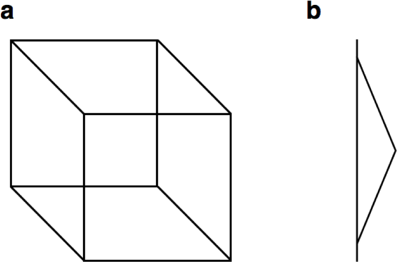
The downside of the hypothesis is that it does not explain the well-known Necker cube [22], which is the orthographic projection of a slanted cube. The linear-perspective hypothesis predicts that all faces of the Necker cube should be perceived in the fronto-parallel plane, because all lines relevant to the hypothesis are parallel to each other (Figure 1a). Yet, Necker cubes are perceived as three-dimensional cubes, albeit that the cubes flip in depth and slant. The bistability of the Necker cube is impressive, because it survives non-zero disparities between the front- and back-side during binocular vision. Bistability is even seen in random-dot versions [23]. Necker cubes are unexplained three-dimensional shapes, because it is not clear which cues indicate the bi-stable shape. As Gregory [24] observed: “we can produce depth with no depth clues, as with a drawing of a wire cube, a Necker cube. Though lacking depth clues—there is no perspective as the sides are parallel—it is seen as three dimensional, and it clearly flips in depth”. Symmetry is a clue, nowadays usually called a cue, which Gregory did not consider. A cube contains nine planes of mirror symmetry. Sawada [25] showed that human observers are reliable at discriminating symmetric from non-symmetric shapes from just a single non-symmetric picture. However, Necker cubes (Figure 1a) contain two (oblique) axes of mirror symmetry in the picture. Symmetry as such does not seem sufficient to explain the perceptual dominance of a bi-stable cube, because even irregular Necker cubes are perceived as 3D [26].
Necker cubes may contain local cues that specify the slant of surfaces relative to the observer. The angles of Necker cubes, which are oblique in the plane of the picture, are perceived as right angles of the cube. The question arises whether orthogonality, defined as the preference for a right-angle interpretation of oblique angles, is the assumption made by the visual system that renders the Necker cube both three-dimensional and bi-stable. Saunders and Backus [27] reported evidence that the orthogonality assumption contributed to the slant of surfaces in certain conditions. Their stimuli, however, also contained skew symmetry, i.e., skewed surfaces in pictures that can be understood as projections of symmetric surfaces, oriented non-perpendicularly to the observer. Saunders and Knill [28] provided convincing evidence that skew in association with an assumption of symmetry is a strong cue to surface slant. Sawada and Pizlo [29] showed that subjects are good at detecting slanted symmetric shapes in skewed line drawings. Thus, it may be possible that subjects in the experiments of Saunders and Knill [28] did not use the assumption of orthogonality, but instead an assumption of symmetry.
Solutions for the symmetry and orthogonality assumptions co-vary in Necker cubes. Therefore, Necker cubes are not suited for studying the assumptions separately. Figure 1b shows a triangular shape that may look like a triangular flag attached to a vertical pole. The triangle may be perceived as a slanted flag; it may even alternate between two orientations. Mirror symmetry and skew symmetry cannot serve as cues to its slant, because the triangle is symmetric about the horizontal plane in any orientation about the vertical pole. The assumption of orthogonality, however, yields distinct slant interpretations. For triangular shapes as shown in Figure 1a, the oblique angle in combination with an assumption of orthogonality is the only cue to slant. The cue is dubbed the oblique-angle cue.
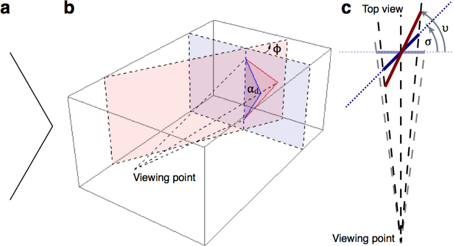
Figure 2a shows an obtuse angle for which the assumption of orthogonality specifies a particular slant differing from that of the screen. The assumption of orthogonality specifies a slant ϕ given the requirement that the retinal image of the right angle must be indistinguishable from that produced by the obtuse angle imaged on the screen (Figure 2b). An implicit assumption is that the angular shape is symmetric about the horizontal plane. A potential problem in estimating slant from oblique angles or any other perspective cue is that many other cues contribute to the perception of slant. Established cues are the blur and brightness of lines, binocular disparity (in the case of binocular viewing), ocular vergence and accommodation [30]. Fortunately, these cues have in common that they indicate slant of the physical stimulus and, thus, the screen, but not slant specified by the oblique-angle cue. Together, these cues are dubbed screen cues. Measuring perceived slant as a function of slant ϕ and σ provides the possibility to isolate the contribution of the oblique-angle cue from contributions of the screen cues [21]. The geometry and equations used in this paper are explained in the Supplementary Material Appendix of Erkelens [21].
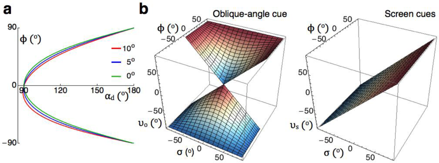
For an obtuse angle as shown in Figure 2a, there is a specific relationship between αd and slant ϕ (Figure 3a). Each obtuse angle is associated with two right angles, one having positive and the other negative slant. For vertices located off the axis of rotation, ϕ is not symmetric about the horizontal axis, because the screen at the vertex is not oriented perpendicularly to the viewing direction when σ = 0. For smaller offsets, ϕ becomes more symmetric until, for vertices placed at the axis, ϕ is described by the symmetric relationship , with ϕ and αd expressed in degrees. This relationship between an oblique angle and slant provides an objective test for the hypothesis that the perceived slant of obtuse angles is based on an assumption of orthogonality.
For both the oblique-angle cue and screen cues, Figure 3b shows the computed relationships between three slants, υ, i.e., slant specified by the shape of the retinal stimulus, ϕ, i.e., slant specified by the shape of the stimulus on the screen, and σ, i.e., slant of the screen. The oblique-angle cue can be understood as a process in the visual system that converts oblique angles in the retinal image into right angles slanted in space. Screen slant σ affects the perceived slant, because slanting by σ transforms αd into an angle αr in the retinal stimulus. For σ = 0°, αr = αd and υo = ϕ, where υo is slant specified by an oblique angle on an assumption of orthogonality (Figure 3b, left graph). Screen cues are related to the physical properties of the picture on the screen, not to what is depicted on the screen. This means that υs, i.e., slant specified by screen cues depends on σ, but not ϕ (Figure 3b, right graph). Arranging slant judgments of subjects as functions of ϕ and σ and comparing these with the predictions shown in Figure 3b provides the possibility to estimate the contribution of the oblique-angle cue and screen cues to the slant perceived of obtuse angles.
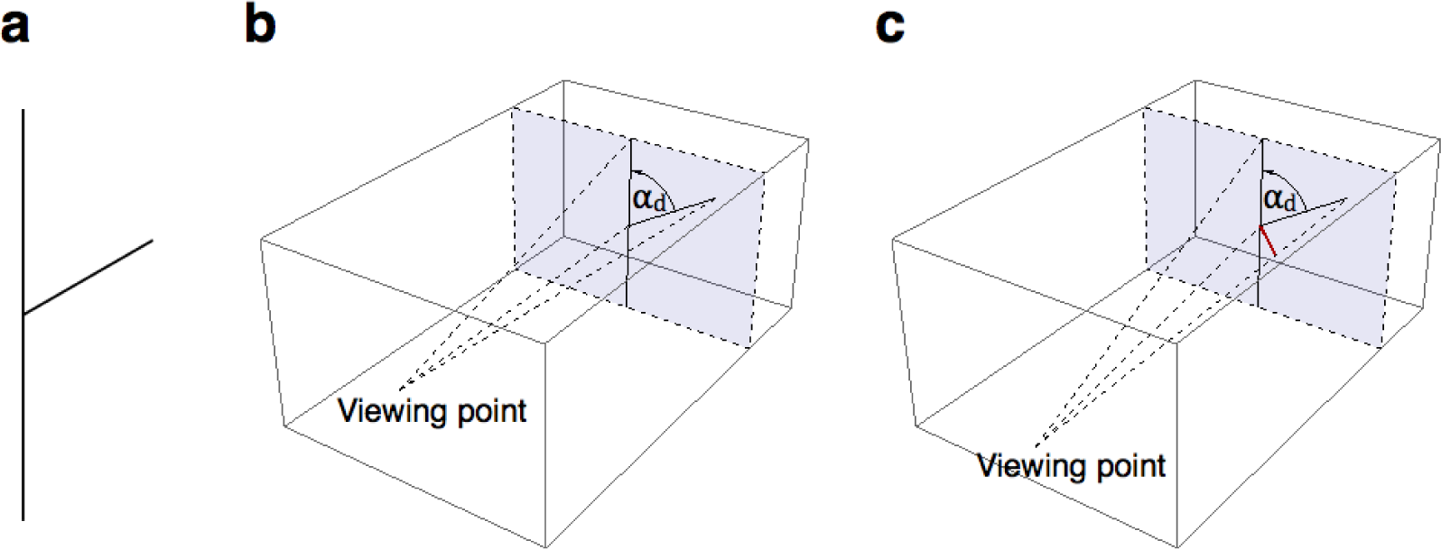
The isosceles triangle of Figure 1b can elicit three alternative 3D percepts. One interpretation will be investigated by using stimuli as shown in Figure 2a. This interpretation uses the implicit assumption that the horizontal plane is a plane of symmetry. Alternatively, the triangle can also be interpreted as a triangle of which one of the angles along the pole is a right angle. There are two mutually exclusive interpretations if the observer assumes that his viewpoint is lower than the triangle. One interpretation is that the upper angle is orthogonal, and the triangle slants away from the observer. In the other interpretation, the lower vertex is orthogonal, and the triangle slants towards the observer. A viewpoint above the triangle yields the reversed combinations of right angle and slant. Here, the implicit assumption is that one of the oblique lines is lying in the horizontal plane. To avoid any confusion due to multiple interpretations, the percepts will be studied by using the even simpler stimulus shown in Figure 4a. The two abutting lines may be perceived to lie in the picture plane (Figure 4b). The assumption of orthogonality is discarded in this interpretation. However, the oblique line may also be perceived as a horizontal line that is slanted relative to the plane of the picture. The assumption of orthogonality is incorporated in this interpretation. Figure 4c explains the 3D geometry of this extremely simple two-line configuration. Slant judgments were measured for the stimulus of Figure 4a to investigate the generality of the assumption of orthogonality.
2. Results
2.1. Slant Judgments for Oblique Triangles
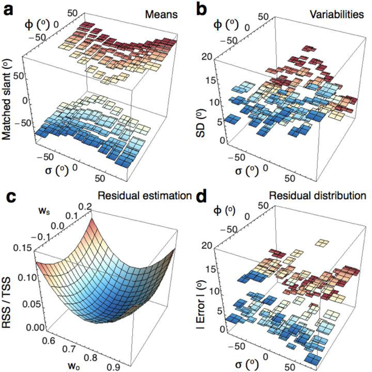
Observers judged the slant of the angles (Figure 2a) by adjusting the slant of the rectangular pad until both slants matched. Figure 5a shows the means and Figure 5b the standard deviations (SDs) for the 99 combinations of ϕ and σ. The distribution of the means shows a striking resemblance with the oblique-angle-cue predictions (Figure 3b). The distribution of the SDs shows little internal structure. All SDs are smaller than 17°.
To estimate the predictive value of the oblique-angle cue and the screen cues, the residual sum of squares was computed as a fraction of the total sum of squares (RSS/TSS) for fits of the models to the mean matched slant results. The oblique-angle cue explained 97% of the data (wo = 0.75) and the screen cue 1% (ws = 0.05). A just slightly better fit was found by a linear combination of the oblique-angle cue and screen cues (Figure 5c). The model combining cue-weights wo = 0.75 and ws = 0.05 gave the best result by explaining 98% of the matched slant.
To estimate confidence intervals for the cue weights, the regression analysis was repeated for matched slant data of individual subjects (Table 1). For the group of six subjects, 95% confidence intervals are about twice as large as one SD. Residual errors computed from the individual data were similar to those computed from the mean data. The one-cue fits show that the oblique-angle cue explained most of the matched data. The addition of the screen cue to the model hardly increased the explanatory power, namely from 95% (res = 0.05; res, residual errors) to 96% (res = 0.04).
To judge the quality of the model predictions in detail, residual errors were computed as functions of ϕ and σ for the optimal cue-weight combination (Figure 5d). SDs (Figure 5b) and absolute residual errors (Figure 5d) are of the same order of magnitude. The simplest explanation for the similar levels of variability is that residual errors reflect between-subject variability. If this explanation is valid, the slant model combining the oblique-angle cue and screen cues with a ratio of nineteen to one fully explains the matched slant.
2.2. The Effective Stimulus for Slant of Symmetric Angles
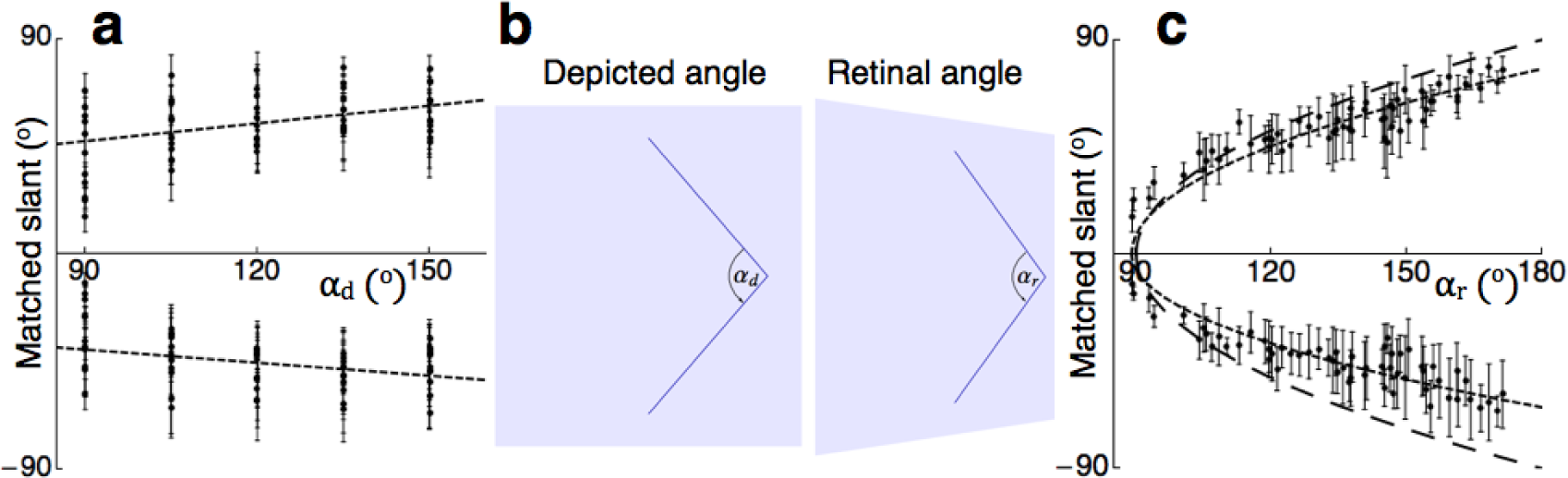
To find the effective stimulus for perceived slant, the matched-slant data shown in Figure 5a,b were re-plotted as a function of αd (Figure 6a).
Linear fits of the data showed small, but significant dependences of matched slant on αd (slopes of 0.31 (F1,328 = 65, p < 0.01) and −0.25 (F1,328 = 40, p < 0.01), respectively). The linear fits, however, only poorly described the data (R2 of 0.16 and 0.11, respectively). The results shown in Figure 6a only poorly resemble the predicted relationship between ϕ and αd (Figure 2a). The predictions were computed, however, for angles αd imaged on a fronto-parallel screen, whereas the matched slants were obtained from angles seen on a screen having various slants. The slant of the screen affected the size of the obtuse angle αr in the retinal image (Figure 5b). The relationship between αd and αr is given by: tan αr = tan αd/cos σ. To find the retinal correlate of slant specified by the oblique-angle cue, the matched slants were re-plotted as a function of αr (Figure 6c). The one-parameter, non-linear model given by matched slant provided good fits (g = 8.2, R2 = 0.96; g = −6.7, R2 = 0.94). The comparison of the gains of the data (±g) to gains specified by the oblique-angle cue shows that the predicted slants were underestimated considerably. The gains of the data were 86% and 70% of the expected gains, respectively.
2.3. The Effective Stimulus for Slant of Asymmetric Angles
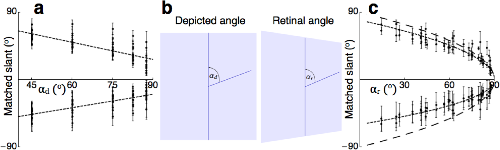
To find the effective stimulus for perceived slant, the matched slants for the oblique line stimuli (Figure 4a) were plotted as a function of αd (Figure 7a). Linear fits to the data showed significant dependences of matched slant on αd (slopes of −0.76 (F1,328 = 289, p < 0.01) and 0.59 (F1,328 = 149, p < 0.01), respectively). The linear fits only moderately described the data (R2 of 0.47 and 0.31, respectively). As for the symmetric angles, the slant of the screen affected the size of the angles αr in the retinal image (Figure 7b). To find the retinal correlate of slant specified by the oblique-angle cue, the matched slants were re-plotted as function of αr (Figure 7c). Linear fits to the data showed significant dependences of matched slant on αr (slopes of −0.67 (F1,328 = 667, p < 0.01) and 0.54 (F1,328 = 304, p < 0.01), respectively). The one-parameter, non-linear model given by matched slant provided good fits (g = 8.4, R2 = 0.95; g = −6.3, R2 = 0.89). Comparison of gains of the data to gains specified by the oblique-angle cue shows that the predicted slants were underestimated considerably again. Gains were 89% and 66% of the expected gains, respectively.
The matched slants of symmetric and asymmetric angles were well described by slants based on an assumption of orthogonality. The general level of underestimation was very similar to that found for slant specified by perspective convergence measured in a recent study [21].
3. Discussion
3.1. Evidence for the Oblique-Angle Cue
The consistency of the slant judgments across stimuli, screen slants and subjects indicates a common underlying principle. Slant judgments of the symmetric angles show that an assumption of orthogonality must be the underlying principle, because these angles do not contain any other cue to slant. The consistency between judgments of symmetric and asymmetric angles suggests that the oblique-angle cue is also the dominant cue for the asymmetric angles. The slant judgments support the claim of Saunders and Backus [27] that in addition to skew asymmetry, oblique angles are a cue to slant. In an earlier study, Perkins [31] already showed that subjects had a preference for orthogonality in judgments of angles. A new element in the current study is that subjects were not asked about the shape of stimuli, but were asked to indicate their slant. The excellent agreement between the slant judgments and slants specified by the oblique-angle cue (Figure 5 and Table 1) indicates that humans prefer the interpretation that oblique angles in the retinal image are produced by right angles of slanted surfaces in the physical world. The ratio of nineteen to one between the cue weights shows that the oblique-angle cue strongly prevailed over the screen cues, including binocular disparity. It may be that the ratio was driven to an upper limit by the subject’s instruction to ignore the slant of the screen as much as possible. The ratio between the cue weights is remarkable, because it shows a virtual complete neglect of all other cues present in the stimuli. Yet, oblique angles in a picture are not always interpreted as right angles. Pictorial cues other than oblique angles must be responsible for oblique-angle interpretations, because non-pictorial cues do not seem to play a role in this.
The dominance of another pictorial cue over screen cues was recently observed for perspective convergence, which was the pictorial cue to slant in simple grid stimuli [21]. There are similarities, as well as a difference between converging lines and oblique angles as cues to slant. What is similar is that slant is underestimated considerably. The underestimation is not explained by competition from screen cues, because the contributions of screen cues appeared to be almost absent. Likewise similar is that both cues are fully based on retinal information and do not require any additional information, such as, for instance, the distance of projection or the distance of viewing. Another similarity between perspective convergence and oblique-angle cues is the degree of precision that is required for the conversion of retinal information into perceived slant. Perspective convergence was found to be a highly precise cue to slant, especially for small angles of convergence [21]. Thresholds for angular differences between line orientations were on the order of a few minutes of arc. Thresholds for the oblique-angle cue show similar characteristics. SDs and residual errors of slant were smaller than 17° over the total ranges of αr and σ measured in the experiments. For angles of αr near 90°, however, SDs were considerably smaller, implying that thresholds for the detection of angular differences near 90° were on the order of tens of minutes of arc. A difference between the two cues is that perspective convergence is an unambiguous cue to slant in that there is a one-to-one relationship between an angle of convergence and the slant that it specifies. Oblique angles are an ambiguous cue to slant. This difference between perspective convergence and oblique angles as cues plays an important role in the bistability of Necker cubes.
3.2. Bistability of Necker Cubes and Cue Combination
Necker cubes are usually perceived as bi-stable, three-dimensional cubes. This is remarkable, because screen cues, as well as linear perspective and image symmetry signal that the retinal shape represents a two-dimensional shape on the screen. Just two cues, namely object symmetry and angular orthogonality, favor a three-dimensional interpretation of the retinal shape. Perceptual dominance of the 3D shape implies that the visual system ignores reliable cues to a 2D shape in favor of ambiguous and, therefore, unreliable cues to 3D shape. The cues are ambiguous, because they are uncertain about the orientation of the cube. This reasoning challenges the view that perceptual judgments derived from cues are weighted by the inverse of the variance of each of the cues [32–36]. Cue combination and maximum-likelihood estimation have been presented as convincing evidence for a probabilistic approach in perception [32,37–42]. Cue combination and weighting may be limited to shapes for which cues signal relatively small differences. Necker cubes illustrate that the visual system can disengage reliable and strong cues, such as binocular disparity and linear perspective, if these cues specify very different 2D shapes. Selective disengagement of cues may be the mechanism that underlies the success of 2D images in ancient, as well as modern civilizations.
3.3. Neural Coding of Slant
In a recent study, I proposed that processing of perspective convergence occurs at an early stage in the visual cortex [21]. The proposal came from agreement between levels of precision measured for orientation discrimination and slant. Similar levels of precision and the fact that slant is seen in stimuli as simple as consisting of only two abutting line elements suggests that the oblique-angle cue is processed early in the visual cortex, too. Neural measurements of high precision made early in the visual cortex argues for the presence of local, neural detectors of slant. Slant detectors using perspective convergence and oblique angles as input would be a logical first stage for the processing of three-dimensional shape in view of the presence of the abundance of neurons selective for the orientation of visual lines and edges in V1 [43–47]. If such detectors indeed exist, the one-to-two relationship between oblique angles and slant implies that positive and negative slants are signaled by separate groups of oblique-angle detectors. The asymmetry in the durations of bistability experienced by a few subjects and the asymmetry between the gains of the fits support separate groups of detectors. The fact that percepts of positive and negative slant do not co-exist could be the result of a process of mutual inhibition between opponent slant detectors. The suggestion for two groups of competing slant detectors fits in nicely with the results from EEG recordings made during viewing of ambiguous Necker cubes and lattices [48–50]. EEG paradigm allowing time-resolved EEG measurement during endogenous perceptual reversals revealed a chain of ERP correlates beginning with an early occipital positivity at around 130 ms (RP, reversal positivity). RP was preceded by a stimulus-size-related P100 at around 100 ms. The RP was percept-related and largely unaffected by stimulus size. The authors concluded that the results indicate that low-level visual processing (related to stimulus size) and high-level processing (related to perceptual reversal) occur in close spatial and temporal vicinity. The characteristics of the suggested oblique-angle detectors would nicely explain the results of Kornmeier and Bach [49]. The two competing groups of detectors receive almost equal input during viewing of ambiguous Necker cubes. The dominance of one percept over the other may result from an imbalance (different initial states, noise, different gains) between the competing groups. Building up of the imbalance to a certain threshold may explain the time delay of 30 ms between P100 and RP.
3.4. Material and Methods
3.4.1. Subjects
The study included 6 subjects (first-year physics students). All were naive with respect to the purpose of the study. All subjects had normal or corrected-to-normal vision and gave informed consent in accordance with the Declaration of Helsinki. The Ethics Committee of the Faculty of Social and Behavioral Sciences of Utrecht University approved the study. The approval is filed under Number FETC14-018.
3.4.2. Stimuli
The stimuli were symmetric, isosceles angles (Figure 2a) constituted by two white (93 cd/m2) lines against a black (approximately 2 cd/m2 in frontal view) background displayed on a TFT (thin-film transistor liquid-crystal display) monitor (21″ LaCie 321, La Cie Ltd., Tigard, OR, USA, 1600 × 1200 pixels, 75 Hz). The display area of the monitor was approximately 43° × 32°. The screen slanted about the (invisible) vertical axis running through the end points of the lines. The vertices were located 10° at the right side from the axis on the front-parallel screen. Five angles were used in which αd was 90°, 105°, 120°, 135° and 150°, respectively. On a fronto-parallel screen, the slants ϕ specified by the oblique-angle cue in these stimuli were 0°, +33°, −48°, +49°, −60°, +61°, −70°, +72° and −77°.
In separate sessions, the perceived slant was estimated in response to the type of stimuli shown in Figure 4a. The length of the vertical line was always 32°, and the horizontal extent of the oblique line was 10°. The acute angles of the stimuli were 45°, 60°, 75°, 82.5° and 87.5° on the fronto-parallel screen. The slants ϕ specified by the oblique-angle cue in these stimuli were 0°, ±64°, ±52°, +37°, ±26° and ±15°.
3.4.3. Experimental Procedure
A chin rest restricted head movements, so that the center of the screen was positioned in the mid-sagittal plane of the head. Viewing was binocular. The setup was placed in a normally lit room, because pictures are usually viewed against visible frames and backgrounds. The monitor was centered on a turntable at a distance (=center of the forehead to the center of the turntable) of 57 cm. A second turntable, centered within a protractor and carrying a vertical rectangular pad (23 × 16 cm), was placed between the center of the monitor and the chin rest at a distance of 21 cm from the forehead. Subjects oriented the pad with both hands to indicate the perceived slant of the stimuli. The vertical distance between the obtuse angles and the upper edge of the pad was about 30°, so that the subjects alternated their fixation between up and far and near and down during the adjustment of the pad. The slant of the screen σ was varied between −75° and 75° in steps of 15°. Combinations of αd and σ were selected in fully randomized order. In order to familiarize the subjects with the task, they ran three pre-trials without a stimulus on the screen. They were asked to match the slant of the screen while they viewed the screen binocularly. The results of pre-trials were evaluated, and the trials repeated if the settings were too inaccurate. The purpose of practicing was to ensure that the slant settings reflected perceived slant as much as possible. After some practice, all subjects were able to judge the slants of the screen within error margins of 5° of slant and without a noticeable bias. The viewing condition and method of slant judgment have been tested extensively in a previous study [1]. The subjects were instructed to ignore the slant of the screen in the real experiment and to focus on the slant of the stimuli. They were asked to judge two slants for each stimulus, one having a positive slant and the other one having a negative slant. All of the subjects were able to make both judgments. They made the judgments one after the other in an individually preferred order. Three subjects reported that the bistability of the slants was asymmetric in time. The periods of seeing one slant lasted a long time, whereas the other slant was seen for just short intervals. All subjects were given ample time to allow accurate judgments.
Acknowledgments
The author thanks Pieter Schiphorst for technical assistance.
Conflicts of Interest
The authors declare no conflict of interest.
References
- Erkelens, C.J. Virtual slant explains perceived slant, distortion and motion in pictorial scenes. Perception 2013, 42, 253–270. [Google Scholar]
- Cook, N.D.; Hayashi, T.; Amemiya, T.; Suzuki, K.; Leumann, L. Effects of visual-field inversions on the reverse-perspective illusion. Perception 2002, 31, 1147–1151. [Google Scholar]
- Cutting, J.E. Rigidity in cinema seen from the front row, side aisle. J. Exp. Psychol 1987, 13, 323–334. [Google Scholar]
- Cutting, J.E. Affine distortions of pictorial space: Some predictions for Goldstein (1987) that la Gournerie (1859) might have made. J. Exp. Psychol 1988, 14, 305–311. [Google Scholar]
- Goldstein, E. Rotation of objects in pictures viewed at an angle. J. Exp. Psychol 1979, 5, 78–87. [Google Scholar]
- Goldstein, E. Spatial layout, orientation relative to the observer, and perceived projection in pictures viewed at an angle. J. Exp. Psychol 1987, 13, 256–266. [Google Scholar]
- Goldstein, E. Geometry or not geometry—Perceived orientation and spatial layout in pictures viewed at an angle. J. Exp. Psychol 1988, 14, 312–314. [Google Scholar]
- Gombrich, E.H. The visual image. Sci. Am 1972, 227, 82–96. [Google Scholar]
- Koenderink, J.J.; van Doorn, A.J.; Kappers, A.M.L.; Todd, J.T. Pointing out of the picture. Perception 2004, 33, 513–530. [Google Scholar]
- Kubovy, M. The Psychology of Perspective and Renaissance Art; Cambridge University Press: Cambridge, UK, 1986. [Google Scholar]
- Papathomas, T.V. Experiments on the role of painted cues in Hughes’s reverspectives. Perception 2002, 31, 521–530. [Google Scholar]
- Papathomas, T.V.; Kourtzi, Z.; Welchman, A.E. Perspective-based illusory movement in a flat billboard—An explanation. Perception 2010, 39, 1086–1093. [Google Scholar]
- Pirenne, M.H. Optics, Painting and Photography; Cambridge University Press: Cambridge, UK, 1970. [Google Scholar]
- Rogers, B.; Gyani, A. Binocular disparities, motion parallax, and geometric perspective in Patrick Hughes’s “reverspectives”: Theoretical analysis and empirical findings. Perception 2010, 39, 330–348. [Google Scholar]
- Todorovic, D. Is pictorial perception robust? the effect of the observer vantage point on the perceived depth structure of linear-perspective images. Perception 2008, 37, 106–125. [Google Scholar]
- Cook, N.D.; Yutsudo, A.; Fujimoto, N.; Murata, M. Factors contributing to depth perception: Behavioural studies on the reverse perspective illusion. Spati. Vis 2008, 21, 397–405. [Google Scholar]
- Papathomas, T.V. Art pieces that “move” in our minds: An explanation of illusory motion based on depth reversal. Spat. Vis 2007, 21, 79–95. [Google Scholar]
- Vishwanath, D.; Girshick, A.R.; Banks, M.S. Why pictures look right when viewed from the wrong place. Nat. Neurosci 2005, 8, 1401–1410. [Google Scholar]
- Koenderink, J.J.; van Doorn, A.J. Gauge fields in pictorial space. SIAM J. Imag. Sci 2012, 5, 1213–1233. [Google Scholar]
- Koenderink, J.J.; van Doorn, A.J.; Wagemans, J. Depth. I-Perception 2011, 2, 541–564. [Google Scholar]
- Erkelens, C.J. Computation and measurement of slant specified by linear perspective. J. Vis 2013, 13, 1–11. [Google Scholar]
- Necker, L.A. Observations on some remarkable optical phaenomena seen in Switzerland; and on an optical phaenomenon which occurs on viewing a figure of a crystal or geometrical solid. Lond. Edinb. Philos. Mag. J. Sci 1832, 1, 329–337. [Google Scholar]
- Erkelens, C.J. Contribution of disparity to the perception of 3D shape as revealed by bistability of stereoscopic Necker cubes. Seeing Perceiving 2012, 25, 561–576. [Google Scholar]
- Gregory, R.L. Distortion. In Seeing through Illusions; Oxford University Press: Oxford, UK, 2009; pp. 159–208. [Google Scholar]
- Sawada, T. Visual detection of symmetry of 3D shapes. J. Vis 2010, 10, 1–22. [Google Scholar]
- Kanizsa, G. Organization in Vision; Praeger: New York, NY, USA, 1979. [Google Scholar]
- Saunders, J.A.; Backus, B.T. Both parallelism and orthogonality are used to perceive 3D slant of rectangles from 2D images. J. Vis 2007, 7, 1–11. [Google Scholar]
- Saunders, J.A.; Knill, D.C. Perception of 3D surface orientation from skew symmetry. Vis. Res 2001, 41, 3163–3183. [Google Scholar]
- Sawada, T.; Pizlo, Z. Detection of skewed symmetry. J. Vis 2008, 8, 1–18. [Google Scholar]
- Landy, M.S.; Maloney, L.T.; Johnston, E.B.; Young, M. Measurement and modeling of depth cue combination: In defense of weak fusion. Vis. Res 1995, 35, 389–412. [Google Scholar]
- Perkins, D.N. How good a bet is good form? Perception 1976, 5, 393–406. [Google Scholar]
- Ernst, M.O.; Banks, M.S. Humans integrate visual and haptic information in a statistically optimal fashion. Nature 2002, 415, 429–433. [Google Scholar]
- Hillis, J.M.; Watt, S.J.; Landy, M.S.; Banks, M.S. Slant from texture and disparity cues: Optimal cue combination. J. Vision 2004, 4, 967–992. [Google Scholar]
- Jacobs, R.A. Optimal integration of texture and motion cues to depth. Vis. Res 1999, 39, 3621–3629. [Google Scholar]
- Knill, D.C. Ideal observer perturbation analysis reveals human strategies inferring surface orientation from texture. Vis. Res 1998, 38, 2635–2656. [Google Scholar]
- Van Beers, R.J.; Sittig, A.C.; Denier van der Gon, J.J. Integration of proprioceptive and visual position-information: An experimentally supported model. J. Neurophysiol 1999, 81, 1355–1364. [Google Scholar]
- Ernst, M.O.; Bülthoff, H.H. Merging the senses into a robust percept. Trends Cogn. Sci 2004, 8, 162–169. [Google Scholar]
- Hillis, J.M.; Ernst, M.O.; Banks, M.S.; Landy, M.S. Combining sensory information: Mandatory fusion within, but not between, senses. Science 2002, 298, 1627–1630. [Google Scholar]
- Knill, D.C. Robust cue integration: A Bayesian model and evidence from cue-conflict studies with stereoscopic and figure cues to slant. J. Vis 2007, 7, 1–24. [Google Scholar]
- Mamassian, P.; Landy, M.S. Observer biases in the 3D interpretation of line drawings. Vis. Res 1998, 38, 2817–2832. [Google Scholar]
- Pouget, A.; Beck, J.M.; Ma, W.J.; Latham, P.E. Probabilistic brains: Knowns and unknowns. Nat. Neurosci 2013, 16, 1170–1178. [Google Scholar]
- Welchman, A.E.; Deubelius, A.; Conrad, V.; Bülthoff, H.H.; Kourtzi, Z. 3D shape perception from combined depth cues in human visual cortex. Nat. Neuroscie 2005, 8, 820–827. [Google Scholar]
- Blasdel, G.G.; Salama, G. Voltage-sensitive dyes reveal a modular organization in monkey striate cortex. Nature 1986, 321, 579–585. [Google Scholar]
- Bonhoeffer, T.; Grinvald, A. Iso-orientation domains in cat visual cortex are arranged in pinwheel-like patterns. Nature 1991, 353, 429–431. [Google Scholar]
- Hubel, D.H.; Wiesel, T.N. Functional architecture of macaque monkey visual cortex. Proc. R. Soc. Lond. B 1977, 198, 1–59. [Google Scholar]
- Ohki, K.; Chung, S.; Ch’ng, Y.H.; Kara, P.; Reid, R.C. Functional imaging with cellular resolution reveals precise micro-architecture in visual cortex. Nature 2005, 433, 597–603. [Google Scholar]
- Ohki, K.; Chung, S.; Kara, P.; Hübener, M.; Bonhoeffer, T.; Reid, R.C. Highly ordered arrangement of single neurons in orientation pinwheels. Nature 2006, 442, 925–928. [Google Scholar]
- Kornmeier, J.; Bach, M. The Necker cube—An ambiguous figure disambiguated in early visual processing. Vis. Res 2005, 45, 955–960. [Google Scholar]
- Kornmeier, J.; Bach, M. Ambiguous figures—What happens in the brain when perception changes but not the stimulus. Front. Hum. Neurosci 2012, 6, 1–22. [Google Scholar]
- Kornmeier, J.; Pfaffle, M.; Bach, M. Necker cube: Stimulus-related (low-level) and percept-related (high-level) EEG signatures early in occipital cortex. J. Vis 2011, 11. [Google Scholar] [CrossRef]


| Number of Cues
| |||||
|---|---|---|---|---|---|
| One | Two | ||||
| cue | w | res | cue | w | res |
| O | 0.75 (±0.08) | 0.05 (±0.02) | O | 0.75 (±0.08) | 0.04 (±0.01) |
| S | 0.04 (±0.03) | 0.99 (±0.01) | S | 0.04 (±0.03) | |
© 2015 by the authors; licensee MDPI, Basel, Switzerland This article is an open access article distributed under the terms and conditions of the Creative Commons Attribution license (http://creativecommons.org/licenses/by/4.0/).
Share and Cite
Erkelens, C.J. Evidence for Obliqueness of Angles as a Cue to Planar Surface Slant Found in Extremely Simple Symmetrical Shapes. Symmetry 2015, 7, 241-254. https://doi.org/10.3390/sym7010241
Erkelens CJ. Evidence for Obliqueness of Angles as a Cue to Planar Surface Slant Found in Extremely Simple Symmetrical Shapes. Symmetry. 2015; 7(1):241-254. https://doi.org/10.3390/sym7010241
Chicago/Turabian StyleErkelens, Casper J. 2015. "Evidence for Obliqueness of Angles as a Cue to Planar Surface Slant Found in Extremely Simple Symmetrical Shapes" Symmetry 7, no. 1: 241-254. https://doi.org/10.3390/sym7010241